www.atmos-chem-phys.net/17/1037/2017/ doi:10.5194/acp-17-1037-2017
© Author(s) 2017. CC Attribution 3.0 License.
Factors controlling black carbon distribution in the Arctic
Ling Qi1,2, Qinbin Li1,2, Yinrui Li3,a, and Cenlin He1,2
1Department of Atmospheric and Oceanic Sciences, University of California, Los Angeles, CA, USA
2Joint Institute for Regional Earth System Science and Engineering, University of California, Los Angeles, CA, USA 3School of Physics, Peking University, Beijing, China
anow at: Department of Atmospheric Sciences, University of Illinois Urbana-Champaign, Champaign, IL, USA Correspondence to:Ling Qi ([email protected])
Received: 5 August 2016 – Published in Atmos. Chem. Phys. Discuss.: 10 August 2016 Revised: 16 December 2016 – Accepted: 21 December 2016 – Published: 23 January 2017
Abstract.We investigate the sensitivity of black carbon (BC) in the Arctic, including BC concentration in snow (BCsnow,
ng g−1)and surface air (BC
air, ng m−3), as well as emissions,
dry deposition, and wet scavenging using the global three-dimensional (3-D) chemical transport model (CTM) GEOS-Chem. We find that the model underestimates BCsnowin the
Arctic by 40 % on average (median=11.8 ng g−1).
Natu-ral gas flaring substantially increases total BC emissions in the Arctic (by ∼70 %). The flaring emissions lead to up to
49 % increases (0.1–8.5 ng g−1)in Arctic BC
snow,
dramati-cally improving model comparison with observations (50 % reduction in discrepancy) near flaring source regions (the western side of the extreme north of Russia). Ample obser-vations suggest that BC dry deposition velocities over snow and ice in current CTMs (0.03 cm s−1in the GEOS-Chem)
are too small. We apply the resistance-in-series method to compute a dry deposition velocity (vd)that varies with
lo-cal meteorologilo-cal and surface conditions. The resulting ve-locity is significantly larger and varies by a factor of 8 in the Arctic (0.03–0.24 cm s−1), which increases the fraction of dry to total BC deposition (16 to 25 %) yet leaves the to-tal BC deposition and BCsnowin the Arctic unchanged. This
is largely explained by the offsetting higher dry and lower wet deposition fluxes. Additionally, we account for the ef-fect of the Wegener–Bergeron–Findeisen (WBF) process in mixed-phase clouds, which releases BC particles from con-densed phases (water drops and ice crystals) back to the in-terstitial air and thereby substantially reduces the scavenging efficiency of clouds for BC (by 43–76 % in the Arctic). The resulting BCsnow is up to 80 % higher, BC loading is
con-siderably larger (from 0.25 to 0.43 mg m−2), and BC
life-time is markedly prolonged (from 9 to 16 days) in the
Arc-tic. Overall, flaring emissions increase BCair in the Arctic
(by∼20 ng m−3), the updatedvdmore than halves BCair(by ∼20 ng m−3), and the WBF effect increases BCair by 25–
70 % during winter and early spring. The resulting model simulation of BCsnowis substantially improved (within 10 %
of the observations) and the discrepancies of BCairare much
smaller during the snow season at Barrow, Alert, and Summit (from−67–−47 % to−46–3 %). Our results point toward an
urgent need for better characterization of flaring emissions of BC (e.g., the emission factors, temporal, and spatial dis-tribution), extensive measurements of both the dry deposi-tion of BC over snow and ice, and the scavenging efficiency of BC in mixed-phase clouds. In addition, we find that the poorly constrained precipitation in the Arctic may introduce large uncertainties in estimating BCsnow. Doubling
precipita-tion introduces a positive bias approximately as large as the overall effects of flaring emissions and the WBF effect; halv-ing precipitation produces a similarly large negative bias.
1 Introduction
forc-ing (Bond et al., 2013, and references therein). Warren and Wiscombe (1985) highlighted the climate effect of fallen soot from “smokes” for a nuclear war scenario, which reduced the surface reflectivity of snow and sea ice in the Arctic. Mea-surements by Clarke and Noone (1985) showed that there was ample amount of BC in the Arctic snow to exert cli-mate impacts in the region. Using observations of BCsnow,
Hansen and Nazarenko (2004) quantified, for the first time, the albedo reduction due to BC deposition on snow and ice (2.5 % on average) across the Arctic. The snow-albedo effect of BC in the Arctic has since received wide attention. Numer-ous studies have examined the snow-albedo change in this re-gion due to BC deposition (Jacobson, 2004; Marks and King, 2013; Namazi et al., 2015; Tedesco et al., 2016) and esti-mated the associated surface BC snow-albedo radiative forc-ing to be substantial (0.024–0.39 W m−2)in the Arctic (Bond et al., 2013, and references therein; Flanner, 2013; Jiao et al., 2014; Namazi et al., 2015), comparable to the forcing of tro-pospheric ozone in springtime Arctic (0.34 W m−2, Quinn et
al., 2008). BC deposited on snow and ice is likely to be an im-portant reason for unexpectedly rapid sea-ice shrinkage in the Arctic (Koch et al., 2009; Goldenson et al., 2012; Stroeve et al., 2012). Widespread surface melting of the Greenland Ice Sheet was attributed to rising temperatures and reductions in surface albedo resulting from deposition of BC from North-ern Hemisphere forest fires (Keegan et al., 2014; Tedesco et al., 2016).
To better constrain the radiative forcing and the associ-ated uncertainties of the BC snow-albedo effect in the Arc-tic, it is imperative to improve the diagnosis and predic-tion of BCsnow in the region. Previous studies found large
discrepancies between modeled and observed BCsnow (up
to a factor of 6) in the Arctic (e.g., Flanner et al., 2007; Koch et al., 2009). A comprehensive survey of BCsnow
ob-servations across the Arctic (∼1000 snow samples) by
Do-herty et al. (2010) provided a unique opportunity to constrain BCsnow in the region. Bond et al. (2013) compared results
of BCsnow from the Community Atmospheric Model
ver-sion 3.1 (CAM3.1) (Flanner et al., 2009) and the Goddard Institute of Space Studies (GISS) model (Koch et al., 2009) with the observations from Doherty et al. (2010), averaged over the eight Arctic sub-regions (Fig. 1) as defined by Do-herty et al. (2010). The resulting ratio of modeled to observed BCsnow (sub-regional means) was 0.6–3.4 for CAM3.1 and
0.3–1.6 for GISS. Jiao et al. (2014) found large discrepan-cies in BCsnow (up to a factor of 6) between results from
the Aerosol Comparisons between Observations and Mod-els (AeroCom; http://aerocom.met.no/) and the Doherty et al. (2010) observations. They also found large variations in BC deposition fluxes among the AeroCom models. Jiao et al. (2014) further pointed out that BC transport and deposi-tion processes are more important for differences in simu-lated BCsnowthan differences in snow meltwater scavenging
rates or emissions in models.
Studies have shown that Arctic atmospheric BC on av-erage cools the surface due to surface dimming, while BC in the lower troposphere warms the surface with a climate sensitivity (surface temperature change per unit forcing) of 2.8±0.5 K W−1m2due to low clouds and sea-ice feedbacks
that amplify the warming (e.g., Flanner, 2013). This sen-sitivity is a factor of 2 larger than that of the BC snow-albedo feedback (1.4±0.7 K W−1m2, Flanner, 2013), a
fac-tor of 4 larger than that of CO2 (0.69 K W−1m2, Bond et
al., 2013), and much larger than that of tropospheric ozone (0.2 K W−1m2; Shindell and Faluvegi, 2009). However, es-timates of BCair in the Arctic are associated with large
un-certainties (Textor et al., 2006, 2007; Koch et al., 2009; Liu et al., 2011; Browse et al., 2012; Sharma et al., 2013). In general, current models successfully reproduced the decadal declining trends observed at the surface sites Barrow, Alert, and Zeppelin (Sharma et al., 2004, 2006, 2013; Eleftheri-adis et al., 2009), but failed to reproduce the seasonal cy-cles of BCairobserved at the aforementioned sites, with large
underestimates during the Arctic haze season (Textor et al., 2006, 2007; Koch et al., 2009; Liu et al., 2011; Browse et al., 2012; Sharma et al., 2013; Eckhardt et al., 2015). Specif-ically, mean BCair during January to March was
underesti-mated by about a factor of 2 for the mean of all models, al-though the discrepancy is up to a factor of 27 for individual models (Eckhardt et al., 2015). The low biases are likely due to uncertainties associated with estimates of BC emissions in Russia (Huang et al., 2015), treatments of BC aging in the models (Liu et al., 2011; He et al., 2016), excessive dry de-position of BC (Huang et al., 2010; Liu et al., 2011), wet scavenging of BC (Koch et al., 2009; Huang et al., 2010; Bourgeois and Bey, 2011; Liu et al., 2011), or overly effi-cient vertical mixing (Koch et al., 2009). Studies (Wang et al., 2011; Huang et al., 2015) have pointed out that the low biases of BCair during the Arctic haze season are partially
due to uncertainties in the estimates of BC emissions in Rus-sia, resulted from biases in both BC emission rates and spa-tial distributions. A likely missing source of BC emissions in Russia is natural-gas-flaring emissions, most of which clus-ter in the wesclus-tern side of the extreme north of Russia (Stohl et al., 2013). Although in totality gas-flaring emissions are a rather small fraction of global BC emissions, their proxim-ity to the Arctic can conceivably result in a disproportion-ately large impact. Dry deposition of BC on snow and ice is yet another poorly understood and quantified process. Ob-servations show thatvdover snow- and ice-covered surfaces
vary by orders of magnitude (0.01–1.52 cm s−1; Hillamo et al., 1993; Bergin et al., 1995; Nilsson and Rannik, 2001; Gronlund et al., 2002; Held et al., 2011; Wang et al., 2014). Current chemical transport models (CTMs) tend to assume uniform and low dry deposition velocities over such surfaces to capture the high surface BCairduring the Arctic haze
sea-son (Wang et al., 2011; Sharma et al., 2013). For instance, Wang et al. (2011) used a uniformvd of 0.03 cm s−1 over
mea-0.01 0.02 0.05 0.1 0.2 0.5 1 2 5 8 Denali
Barrow
Alert
Zeppelin Summit
Denali
Barrow
Alert
Zeppelin Summit
Gg yr
Russia Tromsø Canadian sub-Arctic Alaska
Ny-Ålesund
Canadian Arctic
Arctic ocean
Greenland
-1
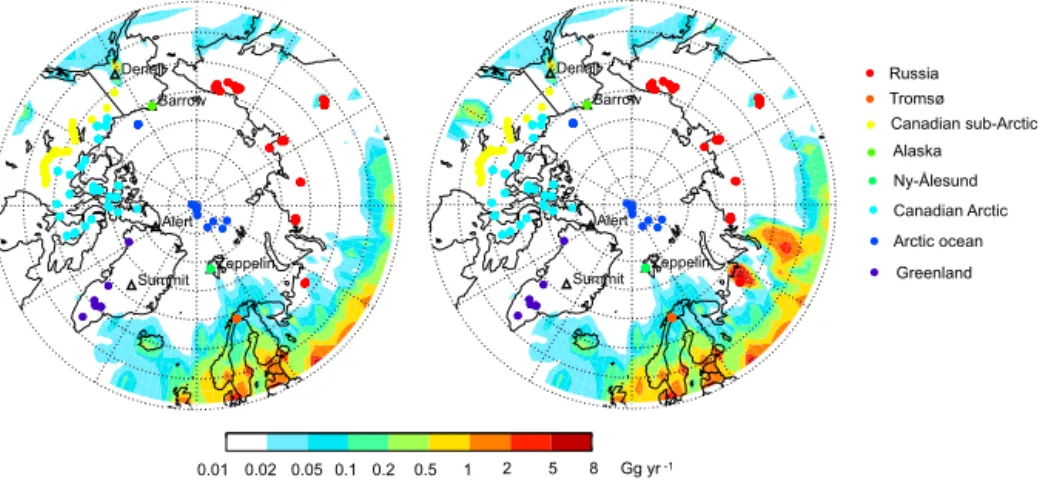
Figure 1.Annual BC emissions (Gg yr−1)in the Arctic in experiment A (left panel) and experiments B, C, and D (right panel). Also shown
are in situ BC measurement stations (open triangles) and snow sample locations (solid circles). The eight sub-regions of the Arctic as defined in Doherty et al. (2010) are color-coded. See text for details.
surements during the Arctic haze season. However, this value is probably too low for snow-covered land surfaces with larger roughness length. Additionally, observations show that BC scavenging efficiency in clouds varies from 0.06 to 0.7 depending on liquid water contents, temperature, and ice mass fraction because of the Wegener–Bergeron–Findeisen (WBF) process in mixed-phase clouds (Cozic et al., 2007; Verheggen et al., 2007). However, in most of the current Ae-roCom models, BC scavenging is poorly treated (Wang et al., 2011; Bourgeois and Bey, 2011) or entirely missing (Liu et al., 2011) in mixed-phase clouds, which cover the Arctic in ∼40 % of the time through a whole year (Zhang et al.,
2010). For example, BC scavenging in mixed-phase clouds was treated the same as that in warm clouds in the GEOS-Chem (Wang et al., 2011). In ECHAM5-HAM2, BC scav-enging efficiency in mixed-phase clouds was set up as 0.06, the lowest observed value in those clouds (Bourgeois and Bey, 2011).
Constraining individual processes of BC is often challeng-ing. Therefore, our focus is more geared toward highlighting missing processes or ones that were previously unaccounted for in governing BC in the Arctic, particularly BC deposition in the region. We first examine and incorporate gas-flaring emissions of BC, which was missing in previous emission es-timates yet account for a large fraction of BC emissions in the Arctic as suggested by Stohl et al. (2013) (Sect. 4.1). We then discuss and improve the simulation of vdfor BC over snow
and ice, which varies by orders of magnitude but was treated as a uniform value by previous studies (Sect. 4.2). We then analyze BC wet scavenging efficiency in mixed-phase clouds accounting for effects of WBF (Sect. 4.3). Finally, we esti-mated the sensitivity of BCsnowto precipitation in the Arctic
(Sect. 4.4). We also use BCairas an additional constraint of
these simulations.
2 BC observations in the Arctic 2.1 Measurements of BC in snow
The most comprehensive measurements of BCsnowwere in
eight sub-regions in the Arctic: Alaska, Arctic Ocean, Cana-dian Arctic, CanaCana-dian sub-Arctic, Greenland, Russia, Ny-Ålesund, and Tromsø, mostly from March to May during 2005–2009 (Doherty et al., 2010; data available at http:// www.atmos.washington.edu/sootinsnow/). Samples were for full snowpack depth and the sampling sites are shown in Fig. 1 (color-coded by the sub-regions). These observations provide a reasonable constraint on Arctic-wide annual mean radiative effect from BC deposited in snow (Jiao et al., 2014). Doherty et al. (2010) measured the light absorp-tion of impurity in snow samples using the integrating sphere/integrating sandwich optical method and derived equivalent, maximum, and estimated BCsnow using the
wavelength-dependent absorption of BC and non-BC frac-tions (Doherty et al., 2010). We use here the estimated BCsnow. The largest sources of uncertainty stem from
un-certainties of BC mass absorption cross section (MAC), BC absorption Ångstrom exponent (ÅBC), and non-BC
absorp-tion Ångstrom exponent (Ånon−BC)constituents. Doherty et al. (2010) used MAC=6.0 mg2g−1 (at 500 nm), the MAC
of their calibration filters. Using MAC=7.5 mg2g−1 (at
500 nm) as recommended by Bond and Bergstrom (2006) would increase the estimated BCsnowby∼25 %. Doherty et
al. (2010) used ÅBC=1.0 (range of 0.8–1.9) and Ånon−BC= 5.0 (range of 3.5–7.0) in their derivation and estimated a
50 % error in the estimated BCsnow. Additional
uncertain-ties include instrumental uncertainty (≤11 %), under-catch
correction (±15 %), and loss of aerosol to plastic flakes in
the collection bags (−20 %) for samples from western
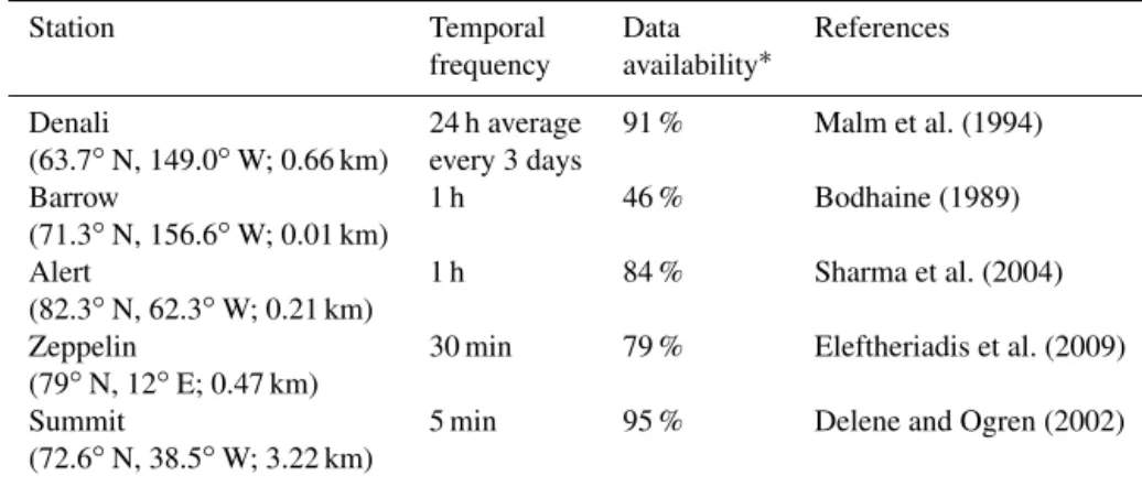
Table 1.Measurements of BC in surface air in the Arctic.
Station Temporal Data References
frequency availability∗
Denali 24 h average 91 % Malm et al. (1994)
(63.7◦N, 149.0◦W; 0.66 km) every 3 days
Barrow 1 h 46 % Bodhaine (1989)
(71.3◦N, 156.6◦W; 0.01 km)
Alert 1 h 84 % Sharma et al. (2004)
(82.3◦N, 62.3◦W; 0.21 km)
Zeppelin 30 min 79 % Eleftheriadis et al. (2009)
(79◦N, 12◦E; 0.47 km)
Summit 5 min 95 % Delene and Ogren (2002)
(72.6◦N, 38.5◦W; 3.22 km)
∗Ratio of available to total data (including available and missing data).
2.2 Measurements of BC in surface air
In situ measurements of BCairfrom 2007 to 2009 are
avail-able at five sites within the Arctic Circle (Fig. 1): De-nali, AL (63.7◦N, 149.0◦W; 0.66 km above mean sea level, a.s.l.), Barrow, AL (71.3◦N, 156.6◦W; 0.01 km a.s.l.), Alert, Canada (82.3◦N, 62.3◦W; 0.21 km a.s.l.), Summit, Green-land (72.6◦N, 38.5◦W; 3.22 km a.s.l.), and Zeppelin, Nor-way (79◦N, 12◦E; 0.47 km a.s.l.). Data descriptions are shown in Table 1. Denali is part of the Interagency Moni-toring of PROtected Visual Environment (IMPROVE) net-work (Malm et al., 1994; data available at http://vista.cira. colostate.edu/improve/). IMPROVE measurements are made every 3 days and 24 h averages are reported. Thermal Opti-cal Reflectance (TOR) combustion method is used based on the preferential oxidation of organic carbon (OC) and BC at different temperatures (Chow et al., 2004). BC-like products of OC pyrolysis can lead to an overestimate of the BC mass. The uncertainties of the TOR method are difficult to quantify (Park et al., 2003; Chow et al., 1993).
Barrow is part of the NOAA Global Monitoring Division (GMD) network, where BC light absorption coefficients have been measured from a particle soot absorption photometer (PSAP) since 1997 (Bond et al., 1999; Delene and Ogren, 2002; data available at http://www.esrl.noaa.gov/gmd/aero/ net/). PSAP measures the change in light transmission at three wavelengths (467, 530 and 660 nm) through a filter on which particles are collected. We used the measurements at 530 nm in this study. Site Barrow is about 8 km northeast of the village of Barrow and is less than 3 km southeast of the Arctic Ocean. Given that the site has a prevailing east-northeast wind off the Beaufort Sea, it receives minimal in-fluence from local anthropogenic emissions and is strongly affected by weather in the central Arctic.
BCairat Alert were measured using an aethalometer model
AE-6 with one wavelength operated by Environment Canada (Sharma et al., 2004, 2006, 2013; data available at http: //www.ec.gc.ca/). The instruments measure the attenuation
of light transmitted through particles that accumulate on a quartz fiber filter at 880 nm. Alert, located the furthest north of the five sites on the northeastern tip of Ellesmere Island, is most isolated from continental sources (Hirdman et al., 2010).
The Zeppelin observatory is part of the European Super-sites for Atmospheric Aerosol Research, where BC mass concentrations are also measured by an aethalometer and reported for seven wavelengths (370, 470, 520, 590, 660, 880, and 950 nm) (Eleftheriadis et al., 2009; data available at http://ebas.nilu.no/). We use the 520 nm data. Measurements at site Zeppelin, on the mountain Zeppelin on the island archipelago of Svalbard, were generally considered to rep-resent the free-troposphere conditions (Eleftheriadis et al., 2009).
BC mass concentrations were also measured by an aethalometer at Summit (von Schneidemesser et al., 2009; data available at http://www.esrl.noaa.gov/gmd/aero/net/), on the center of the Greenland glacial ice sheet. The Sum-mit site is at high elevation (3.2 km a.s.l.) and surrounded by flat and homogeneous terrain (Hirdman et al., 2010).
(Hagler et al., 2007) are 19, 15.9, and 20 m2g−1. The uncer-tainty of absorption enhancement by non-BC absorbers (or-ganic carbon and mineral dust) is generally difficult to quan-tify unless the non-BC absorbers contribute more than 40 % of absorption (Petzold et al., 2013).
3 Model description and simulations 3.1 GEOS-Chem simulation of BC
GEOS-Chem is a global three-dimensional (3-D) CTM driven with assimilated meteorology from the Goddard Earth Observing System (GEOS) of the NASA Global Modeling and Assimilation Office. The GEOS-5 meteorological data sets are used to drive model simulation at 2◦ latitude × 2.5◦longitude resolution and 47 vertical layers from the sur-face to 0.01 hPa. The model averages over “polar caps” be-yond ±84◦ to compensate for artificial polar singularities.
Tracer advection is computed every 15 min with a flux-form semi-Lagrangian method (Lin and Rood, 1996). Tracer moist convection is computed using GEOS convective, entrain-ment, and detrainment mass fluxes as described by Allen et al. (1996a, b). Deep convection is parameterized using the relaxed Arakawa–Schubert scheme (Moorthi and Suarez, 1992; Arakawa and Schubert, 1974), and the shallow convec-tion treatment follows Hack (1994). BC aerosols are emit-ted by incomplete fossil fuel and biofuel combustion and biomass burning. We use global BC emissions from Bond et al. (2007) with updated emissions in Asia from Zhang et al. (2009). Biomass-burning emissions are from the Global Fire Emissions Database version 3 (GFEDv3) (van der Werf et al., 2010) with updates for small fires in Randerson et al. (2012). It is assumed that 80 % of the freshly emitted BC aerosols are hydrophobic (Park et al., 2003) and are con-verted to hydrophilic with an e-folding time of 1.15 days,
which yields a good simulation of BC export efficiency in continental outflow (Park et al., 2005). Dry deposition in the model is computed using a resistance-in-series method (We-sely, 1989; Zhang et al., 2001), whereas it assumes a constant aerosolvdof 0.03 cm s−1over snow and ice (see Sect. 3.3).
Wet deposition follows Liu et al. (2001), with updates as de-scribed in Wang et al. (2011).
3.2 Gas-flaring emissions of BC
Gas flaring is the controlled burning of natural gas in petroleum producing areas, particularly in areas lacking gas transportation infrastructure (Elvidge et al., 2009, 2011). It is estimated that 3.5 % of the world’s natural gas is flared (Elvidge et al., 2016) and results in a large amount of green-house gas emissions (13 662.6 Gg of CO2, Bradbury et al.,
2015). Stohl et al. (2013) derived BC emissions from gas flares by multiplying gas-flaring volumes by emission fac-tors. The flaring volumes were estimated using low-light imaging data acquired by the Defense Meteorological
Satel-lite Program (DMSP) (Elvidge et al., 2011). The DMSP es-timates of flared gas volume are based on a calibration de-veloped with a pooled set of reported national gas-flaring volumes and data from individual flares. Derived using lab-based, pilot-lab-based, and field-based approaches, currently available BC emission factors vary by orders of magnitudes (0.0–6.4 g m−3; Fawole et al., 2016). Stohl et al. (2013) de-rived BC emission factor (1.6 g m−3)based upon emission factors of particulate matter from flared gases. The result-ing gas-flarresult-ing emissions (228 Gg yr−1) account for ∼5 % of global anthropogenic emissions (4.8 Tg yr−1; Bond et al., 2007) and∼3 % of global total emissions (8.5 Tg yr−1;
in-cluding anthropogenic emissions from Bond et al., 2007, and Zhang et al., 2009, and biomass-burning emissions from Randerson et al., 2012). However, the largest contributor Russia, contributing ∼30 % to the global flaring volume,
is located in the clean Arctic Circle. About 40 % of BC emissions in the Arctic (115 Gg yr−1)are from gas flaring (48 Gg yr−1), shown in Fig. 1. It is estimated that flaring
emissions contribute 42 % to the annual mean BCairat
sur-face in the Arctic (Stohl et al., 2013). However, to our knowl-edge, no study so far has investigated the contribution of flar-ing emissions to BCsnowin the Arctic. Thus, we included
flar-ing emissions from Stohl et al. (2013, data on flarflar-ing emis-sions are available at http://eclipse.nilu.no upon request) and investigated the contribution of flaring emissions to BCsnow
and BCairin the Arctic in experiment B (Table 2).
3.3 Dry deposition over snow and ice
Nilsson and Rannik (2001) conducted eddy-covariance flux measurements of aerosol number dry deposition in the Arc-tic Ocean and found a meanvdof 0.19 cm s−1over open sea,
0.03 cm s−1over ice floes and 0.03–0.09 cm s−1 over leads
(Table 3). Following Nilsson and Rannik (2001), Fisher et al. (2011) imposedvd=0.03 cm s−1for aerosols over snow
and ice. They found improved agreements of simulated sul-fate with in situ observations in spring and winter in the Arctic. Wang et al. (2011), also imposingvd=0.03 cm s−1
for aerosols over snow and ice, found better agreements for BC at the same stations as used by Fisher et al. (2011). They thus recommended a uniformvd=0.03 cm s−1for
sul-fate and BC over snow and ice. To capture the winter and spring haze, other studies also used relatively lowvd=0.01–
0.07 cm s−1 (Liu et al., 2011; Sharma et al., 2013). These low values, however, are likely too small for snow-covered land surface, where larger roughness lengths reduce the aero-dynamic resistance thereby increasingvd(Gallagher, 2002).
The roughness length is 0.005 m for sea ice and 0.03–0.25 m for snow-covered land surface with grass and scattered obsta-cles (Wieringa, 1980). As a result,vdis larger over a
Table 2.GEOS-Chem simulations of BC in the Arctic.
Experiments A B C D
Anthropogenic Arctic Bond et al. (2007) Bond et al. (2007) and flaring emissions from Stohl et al. (2013)
emissions Asia Zhang et al. (2009)
Rest of world Bond et al. (2007)
Biomass burning GFEDv3 (van der Werf et al., 2010), with updates from Randerson et al. (2012)
BC aging e-folding time 1.15 days
Deposition Dry 0.03 cm s−1over snow/ice and resistance-in-series over all surfaces
and resistance-in-series over other (Wesely, 1989; Zhang et al., 2001)
surfaces (Wang et al., 2011)
Wet Liu et al. (2001) with updates from Wang et al. (2011)
riming: scavenging efficiency for hydrophilic account for both riming and WBF in
BC is 100 % in warm and mixed-phase clouds mixed-phase clouds (Fukuta and Takahashi, 1999;
Verheggen et al., 2007; Cozic et al., 2007)
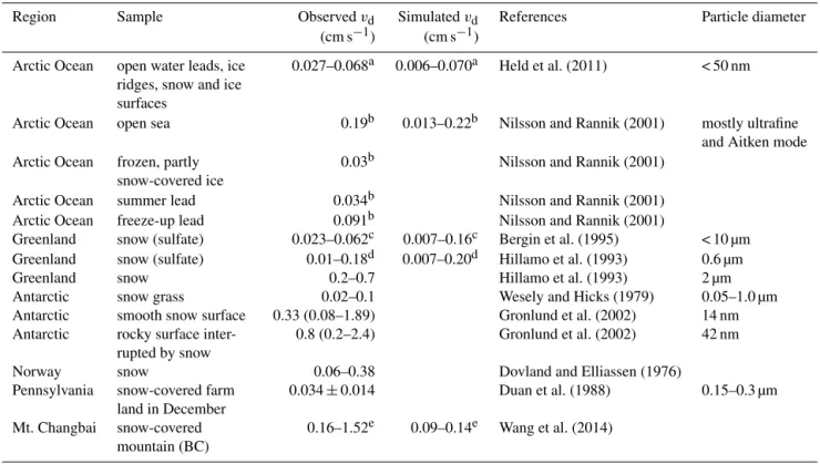
Table 3.Observed and simulated dry deposition velocity (vd)using resistance-in-series method over snow and ice.
Region Sample Observedvd Simulatedvd References Particle diameter
(cm s−1) (cm s−1)
Arctic Ocean open water leads, ice
ridges, snow and ice surfaces
0.027–0.068a 0.006–0.070a Held et al. (2011) < 50 nm
Arctic Ocean open sea 0.19b 0.013–0.22b Nilsson and Rannik (2001) mostly ultrafine
and Aitken mode
Arctic Ocean frozen, partly
snow-covered ice
0.03b Nilsson and Rannik (2001)
Arctic Ocean summer lead 0.034b Nilsson and Rannik (2001)
Arctic Ocean freeze-up lead 0.091b Nilsson and Rannik (2001)
Greenland snow (sulfate) 0.023–0.062c 0.007–0.16c Bergin et al. (1995) < 10 µm
Greenland snow (sulfate) 0.01–0.18d 0.007–0.20d Hillamo et al. (1993) 0.6 µm
Greenland snow 0.2–0.7 Hillamo et al. (1993) 2 µm
Antarctic snow grass 0.02–0.1 Wesely and Hicks (1979) 0.05–1.0 µm
Antarctic smooth snow surface 0.33 (0.08–1.89) Gronlund et al. (2002) 14 nm
Antarctic rocky surface
inter-rupted by snow
0.8 (0.2–2.4) Gronlund et al. (2002) 42 nm
Norway snow 0.06–0.38 Dovland and Elliassen (1976)
Pennsylvania snow-covered farm
land in December
0.034±0.014 Duan et al. (1988) 0.15–0.3 µm
Mt. Changbai snow-covered
mountain (BC)
0.16–1.52e 0.09–0.14e Wang et al. (2014)
aThis range of measurements are medians of dry deposition velocities derived from aerosol number fluxes measured by an eddy-covariance system over different surface
types (open water leads, ice ridges, snow, and ice surfaces) in the Arctic Ocean between 2–10◦W longitude and 87–87.5◦N latitude in late August 2008 (Held et al., 2011). The simulated dry deposition velocities are sampled at the same region during the same time period as observations for BC particles.
bObservations are medians of dry deposition velocities derived from aerosol number fluxes measured by an eddy-covariance system over different surface types in late
July and early August in 1996 in the Arctic Ocean for ultra-fine and Aitken-mode aerosol particles (Nilsson and Rannik, 2001). Simulations are sampled in the same region during the same months as observations in 2008 for BC particles.
cSulfate dry deposition velocities were derived based on particle mass using surrogate surfaces and impactor data at site Summit, Greenland in July 1993 (Bergin et al.,
1995). Simulations are sampled at the same site during July 2008 for BC particles.
dSulfate dry deposition velocities were derived based on particle mass from Cascade impactor at Dye 3 on the south-central Greenland Ice Sheet in March 1989 (Hillamo
et al., 1993). Simulations are sampled at the same site during March 2008 for BC particles.
eThe dry deposition velocities specific to BC particles were derived from measured surface enhancement of BC in snow between two snow events at Changbai Mountain
is problematic. We apply the resistance-in-series method to calculatevdof BC over snow and ice, as a function of
aerody-namic resistance, particle density and size, and surface types (experiment C, Table 2).
We would like to note that most of these observations (Held et al., 2011; Nilsson and Rannik, 2001; Bergin et al., 1995) were from summertime Arctic (June–August) and clean regions (e.g., the Arctic Ocean and Greenland) far from anthropogenic pollution. In addition, most of the vd
mea-surements are for general aerosol particles. The only avail-able dry deposition velocities specific to BC particles are derived from the strong surface enhancement of BCsnow
be-tween two snow events at Mt. Changbai (42.5◦N, 128.5◦E; 0.74 km) in northern China (Table 3). Wang et al. (2014) de-rivedvd=0.16–1.52 cm s−1. Despite uncertainties from
sub-limation (Wang et al., 2014), these measurements suggest that the lowvdused in previous studies (Fisher et al., 2011;
Liu et al., 2011; Wang et al., 2011; Sharma et al., 2013) might underestimate the role of dry deposition during the snow sea-son, particularly near source regions. Wang et al. (2014) con-cluded that dry deposition in the boundary layer may domi-nate over wet deposition (a factor of 5 larger) during the dry season in some regions, particularly near source regions with high BCair. It is thus imperative to obtain measurements of
vdof BC in polluted regions in Russia and northern Europe
in spring, when radiative forcing associated with a BC snow-albedo effect is at a maximum (Flanner, 2013).
3.4 Wegener–Bergeron–Findeisen (WBF) process in mixed-phase clouds
Most AeroCom models (Textor et al., 2006) parameterize rainout rate following Giorgi and Chameides (1986). The rainout ratio is proportional to the precipitation formation rate and mass mixing ratio of BC in a condensed phase in clouds, which is determined by the scavenging efficiency of BC (rscav),
rscav= [BC]condensed
[BC]interstitial+[BC]condensed, (1)
where rscav is the scavenging efficiency and quantifies the
partition of BC aerosols between condensed phase and the interstitial air; [BC]condensed is the mass mixing ratio of BC
in condensed phase, including water drops and ice crystals in clouds, and [BC]interstitial is the mass mixing ratio of BC in
the interstitial air.
The hygroscopicity and size of BC-containing particles are determining factors forrscav(Sellegri et al., 2003;
Hall-berg et al., 1992, 1995). Internal mixing with soluble inor-ganic species enhances therscavfor aged BC particles
(Sel-legri et al., 2003). For instance,rscavis 0.39±0.16 for
BC-containing particles with a diameter smaller than 0.3 µm and a small fraction (38 %) of soluble inorganic material. It in-creases to 0.97±0.02 for particles with a diameter larger
than 0.3 µm and a larger fraction (57 %) of soluble inorganic
material (Sellegri et al., 2003). In addition to particle proper-ties, cloud microphysics and dynamics play a significant role in determiningrscav of BC in mixed-phase clouds
(Hitzen-berger et al., 2000, 2001; Cozic et al., 2007; Hegg et al., 2011). Measuredrscav of BC decreased from 0.60 in liquid
only clouds to 0.05–0.10 in mixed-phase clouds, a reduction of more than a factor of 5 (Cozic et al., 2007; Henning et al., 2004; Verheggen et al., 2007). Such reduction was attributed to the effect of the WBF process (Cozic et al., 2007). In mixed-phase clouds, ice crystals grow at the expense of water drops when the environmental vapor pressure is higher than the saturation vapor pressure of ice crystals but lower than the saturation vapor pressure of water droplets (Wegener, 1911; Bergeron, 1935; Findeisen, 1938). Therefore, BC-containing aerosol particles in water drops, which evaporate to dryness, are released back to the interstitial air and consequentlyrscav
is reduced. Another process, riming (Hegg et al., 2011), in mixed-phase clouds has an opposite effect on BC scaveng-ing. When ice particles fall and collect the water drops along the pathway, the snow particles show rimed structure and the scavenging efficiency remains the same. The riming rate is determined by the terminal velocity of snowflakes, ice crys-tals, and liquid water contents (LWC) in clouds (Fukuta and Takahashi, 1999).
Previously, only the hygroscopicity of BC-containing par-ticles is considered in BCrscavin models (Wang et al., 2011,
and references therein). It is typically assumed that 100 % of hydrophilic BC particles are readily incorporated into cloud drops and all hydrophobic BC particles remain in the inter-stitial air in warm and mixed-phase clouds. This treatment of mixed-phase clouds as liquid phase is likely to overestimate
rscav in phase clouds. In models that include
mixed-phase clouds, assumptions still need to be made aboutrscav.
A uniform scavenging efficiency (0.4 or 0.06) for all mixed-phase clouds has been imposed (Stier et al., 2005; Bourgeois and Bey, 2011), while observations show that BC scavenging efficiency varies dramatically with temperature and ice mass fraction (Cozic et al., 2007; Henning et al., 2004; Verheggen et al., 2007).
In experiment D (Table 2), we discriminate WBF- vs. riming-dominated conditions and parameterize BC scaveng-ing efficiency under the two conditions separately in mixed-phase clouds (248 K <T < 273 K; Garrett et al., 2010). We
assume that riming dominates when temperature is around
−10◦C (261 K <T < 265 K) and LWC is above 1.0 g m−3,
study (Qi et al., 2016). In this study, we focus on the effects of WBF on BC distribution in the Arctic.
3.5 BC concentration in snow
In snow models, such as SNICAR, the initial surface BCsnow
is defined as the ratio of BC deposition to snow precipi-tation (Flanner et al., 2007). Here we approximate BCsnow
using BC deposition flux and snow precipitation rate, fol-lowing Kopacz et al. (2011), Wang et al. (2011), and He et al. (2014a):
[BCsnow]=FBC,dep Fsnow
=Fwet_dep+Fdry_dep
Fsnow , (2)
whereFBC,dep,Fwet_dep, andFdry_dep are total, dry, and wet
deposition flux of BC, andFsnowis the snow precipitation.
The top and bottom snow depth of each sample are provided in the observation data set (Doherty et al., 2010). We accu-mulate snow precipitation (GEOS-5) in the model from the collection date backward until the modeled snow depths, re-spectively, reach the observed top and bottom depths of the snow sample, then the two dates are stored. We use the aver-age BC deposition fluxes and snow precipitation between the two dates to estimate the BCsnowfor the sample. The rate of
snow accumulation at the surface is estimated as snow pre-cipitation flux (kg m−2s−1)over snow density (kg m−3). The observed annual average snow density is 300 kg m−3over the Arctic basin, increasing from 250 kg m−3 in September to 320 kg m−3in May with little geographical variation across the Arctic (Warren et al., 1999; Forsström et al., 2013). We use the annual average snow density in the estimate.
The above estimate of BCsnowignores many processes that
may alter the BC snow concentrations, such as wind redistri-bution of surface snow, sublimation, and meltwater flushing (Doherty et al., 2010, 2013; Wang et al., 2014). Wind re-distribution of surface snow is a subgrid-scale phenomenon. Except for turbulent-scale wind direction and strength, small-scale topography also plays an important role in surface snow distribution; this process is difficult to simulate in global models. Precipitation rate and relative humidity in much of the Arctic are low, so in some areas appreciable (up to 30– 50 %) surface snow is lost to sublimation (Liston and Sturm, 2004). BCsnowat surface can thus be underestimated by our
method. We filtered out snow samples collected during the melting season, so the meltwater flushing has little effect on our estimate.
To reduce the biases in comparison of model results and observations, we organize the observations as follows: (1) observations from March to May in 2007–2009 are used while those from June to August are excluded because our estimate of BCsnowdoes not resolve snow melting, (2) we
ex-clude observations with obvious dust or local wood-burning contaminations as described in Doherty et al. (2010), and (3) we average the observations in the same model grid and snow layer and collected on the same day.
Table 2 summarizes various model simulations in the present study. Experiment A is the standard case. We include gas-flaring emissions in experiment B (Sect. 3.2). Contrast-ing experiments B and A thus offer insights to the contri-bution of gas-flaring emissions on BC in the Arctic. Exper-iment C includes the updatedvd (Sect. 3.3) as well as the
gas-flaring emissions. The difference of experiment B and C denotes the effects of updatedvdto BC distribution.
Ex-periment D includes temperature-based WBF parameteriza-tion (Sect. 3.4) as well as the gas flaring andvdupdates. The
effects of WBF to BC in the Arctic are shown by the dif-ference of experiment C and D. Additional simulations are described where appropriate. In our discussion of the results of the model runs, we assume that there is little or no inter-action between each of the updates; i.e., the order in which the processes have been included does not affect the overall results.
4 The effects of gas flares, dry deposition, WBF, and precipitation
We discuss the effects of gas-flaring emissions, dry depo-sition, WBF in mixed-phase clouds, and precipitation on BC distribution in the Arctic in this section. The probabil-ity densprobabil-ity function of observed and GEOS-Chem simulated BCsnowin the Arctic is approximately lognormal (Fig. 2a).
The arithmetic mean of observations is 17.4 ng g−1, larger than the geometric mean of 12.7 ng g−1 and the median of 11.8 ng g−1(see the vertical lines in Fig. 2 and Table 1). The model reproduces the observed distribution, but underesti-mates BCsnowby 40 % (experiment A). By including flaring
emissions (Sect. 4.1), updatingvd(Sect. 4.2), and including
WBF in mixed-phase clouds (Sect. 4.3), the discrepancy is reduced to−10 %. Gas-flaring emissions lower the
discrep-ancy from−40 to −20 % (experiment B). The updatedvd
(experiment C) makes insignificant changes to BCsnowin the
Arctic. WBF (experiment D) further reduces the discrepancy from−20 to−10 %. The resulting BCsnowin the eight
sub-regions agree with observations within a factor of 2. This dis-crepancy is acceptable for global models because it has been suggested that the error due to different spatial sampling of global models (∼200 km) and point observations was up to
160 % (Schutgens et al., 2016). In addition, BCairat the
sur-face and in the free troposphere is sensitive to the above three processes in the Arctic, particularly during winter and spring (see Sect. 4.1–4.3).
4.1 Gas-flaring emissions
−40 −20 0 20 40
0.00
0.01
0.02
0.03
0.04
0.05
Residual
0.1 0.5 5.0 50.0
0.00
0.02
0.04
0.06
0.08
BC in snow (ng g )
Probability density function
Observations Experiment A Experiment B Experiment C Experiment D
−1 (ng g −1)
Probability density function
Figure 2.Probability density function of observed (solid red) and GEOS-Chem simulated (black curves: dotted – experiment A; dashed –
experiment B; dash dotted – experiment C; solid – experiment D; see Table 2 and text for details) BC concentration in snow (ng g−1)in the
Arctic (left panel), medians (vertical lines, left panel), residual errors (model–observation, right panel), and mean residual errors (vertical lines, right panel).
1 2 5 10 20 50 100
1
2
5
10
20
50
100
Observations (ngg )
Simulations
(ng
g
)
● ● ● ●
Experiment A Experiment B Experiment C
Experiment D
● Alaska Arctic Ocean
Canada sub−Arctic
Canadian Arctic Greenland
Ny-Ålesund
Russia
Tromsø
−1
−1
Figure 3.Observed and GEOS-Chem simulated median BC
con-centration in snow (ng g−1)in the eight sub-regions in the Arctic
(see Fig. 1). Solid line is 1:1 ratio line and dashed lines are 1:2 (or
2:1).
sub-regions. The higher BCsnowleads to a significant
reduc-tion in the negative biases (by 20–100 %), except in the Arc-tic Ocean and in Tromsø, where BCsnow is already
overes-timated without flaring emissions (Fig. 3). BCsnowin
Green-land is not affected by gas-flaring emissions. The reason is 2-fold: first, snow samples in Greenland are far from the flares in western Russia, and second, the vertical transport of BC from surface to the upper troposphere is suppressed by the stable atmosphere in the Arctic (Stohl, 2006), resulting in a negligible effect of flaring emissions to BCsnowover
Green-land (above 1.5 km).
The largest enhancement of BCsnow from flaring
emis-sions is in the western side of the extreme north of Russia within the Arctic Circle (by 5.0 ng g−1on average, or, 50 %), which reduces model discrepancy substantially across Russia
(from−50 to−30 %). However, simulated BCsnow is now
too high (by a factor of 2) near the flares (observed value
∼19.3 ng g−1). The overestimate is likely because of
exces-sively large flaring emission estimates. Yet BCsnowis too low
(by a factor of 2) in far fields (observed value∼30.7 ng g−1),
despite a large increase (by 50 %, from 10.5 to 15.5 ng g−1) as a result of flaring emissions.
Flaring emissions are assumed to be proportional to flared gas volumes and emission factors. Errors in estimates of flared volumes in Russia are small (within±5 %, Elvidge et
al., 2009). Estimates of emission factors, on the other hand, are known to have several orders of magnitude uncertainties (Schwarz et al., 2015; Weyant et al., 2016). Given limited ob-servations of BC emission factors from actual flares, Stohl et al. (2013) derived BC emission factor based upon emission factors of particulate matter from flared gases. They used a BC emission factor of 1.6 g m−3, which is more than a fac-tor of 3 higher than that (0.5 g m−3)from a lab experiment on fuel mixtures typical in the oil and gas industry (McEwen and Johnson, 2012). Recent field measurements have suggested an even lower emission factor (0.13±0.36 g m−3)from∼30
individual flares in North Dakota, with an upper bound of 0.57 g m−3(Schwarz et al., 2015; Weyant et al., 2016). These studies found that average BC emission factors for individ-ual flares varied by 2 orders of magnitude and, furthermore, two flares from the same flare stack that were resampled on different days showed different BC emission factors (Weyant et al., 2016). They also pointed out that emission factors are not correlated with ambient temperature, pressure, humidity, flared gas volumes, or gas composition. It is thus imperative that extensive measurements of BC emission factors be made in the flare regions.
some-times above the nighttime boundary layer height of 150– 300 m in the Arctic (Di Liberto et al., 2012). The stack height affects the ventilation, dispersion, deposition, and long-range transport of the emissions. For example, local deposition of BC may be suppressed and downwind long-range transport enhanced when the stacks emitted BC in the free troposphere (Chen et al., 2009). The lack of proper treatment of flare stack height in the model may partially explain the afore-mentioned discrepancies of modeled BCsnow(biased high in
western Russian and low in eastern Russia). Another factor for the underestimate of BCsnow in eastern Russia is likely
local sources, such as domestic wood burning in nearby vil-lages and fishing camps, diesel trucks on the highway, and coal burning in a power plant, which are unaccounted for in the emission inventory (Doherty et al., 2010, Fig. 1). Al-though we filter out samples with strong local contamination, it is conceivable that local emissions still add to the back-ground BCsnowin eastern Russia.
Jiao et al. (2014) have shown that most AeroCom mod-els underestimated BCsnowin Russia and pointed to the
flar-ing emissions as a likely cause. Our model results show that even with flaring emissions, which are likely on the high side, BCsnow is still too low (by 50 %) in eastern Russia.
There-fore, there are likely other factors such as the lack of lo-cal emissions in eastern Russia, weak dry deposition fluxes (Sect. 4.2), and excessively low rates of sublimation of sur-face snow, which contribute to the large model discrepancy in BCsnow.
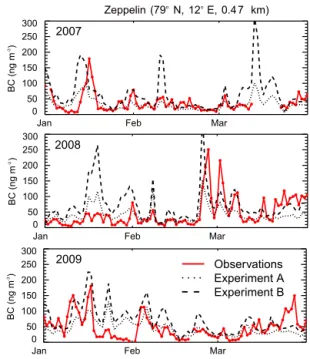
Figure 4 shows observed and GEOS-Chem simulated daily BCairfrom January to March at Zeppelin, a site that is
clos-est to the gas flares in the wclos-estern side of the extreme north of Russia. The inclusion of flaring emissions captures some of the large spikes in the observed BCair, such as those from
late February to March in 2008 and in January 2009. Stohl et al. (2013) found that flaring emissions captured observed large spikes at Zeppelin during a transport event in February 2010 with a high BC/CO ratio, a signature of gas-flaring
emissions (CAPP, 2007). The inclusion of flaring emissions results in enhanced BCair, for instance, in February 2007 and
in January 2008, which are not seen in the observations. This is largely from the lack of temporal variation of flaring emis-sions (Weyant et al., 2016). The temporal variation is, how-ever, difficult to characterize based on the current knowledge of flaring emissions on the western side of the extreme north of Russia (Stohl et al., 2013). Flaring emissions also increase BCair during the snow season (September to April) (by 16–
19 ng m−3)at Barrow and Alert, resulting in substantial re-ductions of discrepancies (from−47 to−15 % at Barrow and −67 to−46 % at Alert) (Fig. 5). The effect of flaring
emis-sions at Denali in the low Arctic is negligible, because the site is outside of the cold Arctic front (around 65–70◦N in Alaska) (Barrie, 1986; Ladd and Gajewski, 2010), which is a strong barrier for the meridional transport of BC (Stohl, 2006). BCair at Summit (3.22 km a.s.l.), which is mostly in
the free troposphere, is not affected by flaring emissions
ei-Jan Feb Mar
0 50 100 150 200 250 300
BC (ng m
-3)
2007
Jan Feb Mar
0 50 100 150 200 250 300
BC (ng m
-3)
2008
Jan Feb Mar
0 50 100 150 200 250 300
BC (ng m
-3)
2009
Zeppelin (79 N, 12 E, 0.4 7 km) o o
Observations Experiment A Experiment B
Figure 4.Observed (red solid) and GEOS-Chem simulated (dotted
– Exp. A, dashed – Exp. B; see Table 2 and text for details) daily BC
concentrations in air (ng m−3
)at Zeppelin from January to March
in 2007–2009.
ther. This is because the vertical transport of BC is sup-pressed by the stable atmosphere during the snow season in the Arctic (Stohl, 2006).
4.2 Dry deposition velocity
It is known that vd of aerosol particles over snow and ice
surfaces strongly depends on particle size, surface types and meteorological conditions and varies by orders of magnitude (Table 3). We estimatevdof BC particles as a function of
par-ticle properties, aerodynamic resistance, and surface types (Sect. 3.3). The results over the Arctic Ocean and Green-land are shown in Table 3, generally within the observed range. At Mt. Changbai, the model result of BCvd(0.09–
0.14 cm s−1)is an order of magnitude lower than that derived by Wang et al. (2014) (0.16–1.52 cm s−1). The resulting dry deposition fluxes are lower than observations by a factor of 5. We attribute the large discrepancies to two factors. First, the point measurements were at a mountainous site with complex terrain and micro-meteorological conditions. Neither can be resolved in a global model (He et al., 2014a). Second, the values reported by Wang et al. (2014) were estimated from relative enhancements of surface BCsnowbetween two snow
events. These estimates are known to have large uncertainties (a factor of 2) from the measured sublimation fluxes and the assumption of snow density (Wang et al., 2014).
Compared to the results of uniformvdof 0.03 cm s−1over
snow and ice, the updatedvdleads to larger dry deposition
rel-BC (ng
m
-3)
Jan Feb Mar Apr May Jun Jul Aug Sep Oct Nov Dec 0
20 40 60 80 100 120 140
BC (ng
m
-3)
Jan Feb Mar Apr May Jun Jul Aug Sep Oct Nov Dec 0
20 40 60 80 100 120 140
BC (ng m
-3)
Jan Feb Mar Apr May Jun Jul Aug Sep Oct Nov Dec 0
20 40 60 80 100 120 140
BC (ng m
-3)
Jan Feb Mar Apr May Jun Jul Aug Sep Oct Nov Dec 0
20 40 60 80 100 120 140
BC (ng m
-3)
Observations Experiment A Experiment B Experiment C Experiment D
Denali (63.7 N, 149. 0 W, 0.66 km) o o Barrow (71.3 N, 156. 6 W,0.01 km) o o
Alert (82.3 o N, 62.3 o W, 0.21 km) Zeppelin (79 N, 12 E, 0.47 km) o o
Summit (72.6 N, 38. 5 W, 3.22 km) o o
Jan Feb Mar Apr May Jun Jul Aug Sep Oct Nov Dec 0
50 100 150 200 250 300
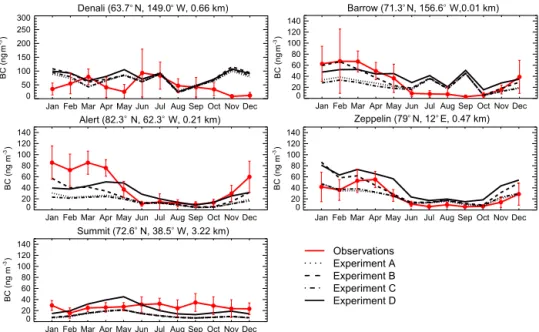
Figure 5.Observed (red solid) and GEOS-Chem simulated (black curves: dotted – Exp. A, dashed – Exp. B, dash dotted – Exp. C, solid –
Exp. D; see Table 2 and text for details) BC concentrations in air (ng m−3)at Denali, Barrow, Alert, Zeppelin, and Summit, averaged for
2007–2009. Also shown are standard deviations of observations (error bars).
atively unchanged total deposition fluxes. Simulated mean BC vd in the eight Arctic sub-regions (Fig. 1) are 0.03–
0.14 cm s−1, which is considerably larger that the uniform
value of 0.03 cm s−1 over snow and ice (Table 5).
Corre-spondingly, thevdare 19–195 % larger in most sub-regions,
with the largest increase in Greenland (by 195 %) and over Russia (by 87 %) (Table 5). We find that BC dry deposi-tion flux is more sensitive tovdin source regions (e.g.,
Rus-sia) than in remote regions, reflecting the high BCair in the
former. A comparable increase in vd of BC (from 0.03 to
0.08 cm s−1)in Russia and Alaska results in vastly differ-ent increases in BC dry deposition flux (87 % in Russia vs. 30 % in Alaska). As expected, larger dry deposition flux de-pletes BCairthereby reducing wet deposition flux but offsets
the reduction in wet deposition. As a result, both total depo-sition flux and BCsnowremain relatively unchanged (< 5 %)
in the eight sub-regions, except in Ny-Ålesund and Tromsø. In these latter two regions, the total deposition fluxes are 10– 15 % smaller. The lower deposition fluxes reflect efficient re-moval of BC aerosols over source regions. BC in Ny-Ålesund and Tromsø are primarily from Europe and Russia, trans-ported isentropically in the cold season (Stohl, 2006; Eleft-heriadis et al., 2009). Rapid dry deposition in these source regions results in enhanced boundary layer removal hence lower BC loadings in air and a reduced boundary layer out-flow (Liu et al., 2011).
The change in the fraction of dry to total deposition has important implications for BC radiative forcing in the Arc-tic. The fraction increases from 19 % (7–33 %) to 26 % (14– 41 %), by 14–73 %, with the largest increase in Russia (from 23 to 40 %) where BC deposition flux and BCsnow are the
largest in the Arctic (Tables 4 and 5). Typically, BC particles removed by dry deposition are externally mixed with snow particles, while those removed by wet deposition are inter-nally mixed with snow particles (Flanner et al., 2009, 2012). Internal mixing of BC with snow/ice particles increases the absorption cross section of BC/snow composites by about a factor of 2 (Flanner et al., 2012). The enhanced absorption further increases the snow-albedo radiative forcing (He et al., 2014b). It is thus conceivable that the larger dry deposi-tion fracdeposi-tion will lead to less internally mixed BC/snow com-posite and lower snow-albedo radiative forcing. This effect is critical before the melting season, because melting might quickly eliminate the differences in the mode of BC deposi-tion. Other post-depositional processes include wind-driven drifting and sublimation (Doherty et al., 2013). The former does not change the fraction of external and internal mixing of BC with snow. The latter might expose BC particles in the internally mixed BC/snow composite and reduce the fraction of internally mixed BC/snow composite. Yet this process oc-curs slowly in a relatively long time.
Unlike BCsnow, BCair is a strong function ofvd,
particu-larly during the snow season. With updatedvd, model results
fail to capture the seasonal cycle of BCairwith dramatic
de-creases during the snow season (by 20–23 ng m−3, 27–68 %) at Barrow, Alert, and Zeppelin (Fig. 5). The decreases at Barrow and Alert are a direct result of larger dry deposi-tion in the boundary layer because of substantially largervd
(0.07 cm s−1, Table 5). At Zeppelin (in Ny-Ålesund), where
vd is only marginally higher (17 %), the large reduction of
BCair(∼40 %) is largely attributed to the suppressed
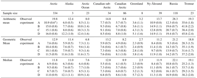
Table 4.Observed and GEOS-Chem simulated BC concentration in snow in the Arctic (ng g−1; see Fig. 1).
Arctic Alaska Arctic Canadian sub- Canadian Greenland Ny-Ålesund Russia Tromsø
Ocean Arctic Arctic
Sample size 334 3 23 34 86 8 39 118 23
Arithmetic Observed 19.8 12.4 8.0 14.8 8.8 3.2 13.7 28.3 19.3
mean experiment A 10.9 (0.6∗) 6.0 (0.5) 8.5 (1.1) 7.7 (0.5) 5.7 (0.7) 3.6 (1.1) 10.9 (0.8) 12.3 (0.4) 35.6 (1.8)
B 15.0 (0.8) 7.7 (0.6) 10.8 (1.4) 9.3 (0.6) 6.7 (0.8) 3.6 (1.1) 14.9 (1.1) 19.6 (0.7) 41.8 (2.2) C 15.1 (0.8) 8.0 (0.6) 10.3 (1.3) 9.1 (0.6) 7.0 (0.8) 4.3 (1.3) 12.8 (0.9) 20.7 (0.7) 38.4 (2.0) D 16.0 (0.8) 12.2 (1.0) 12.4 (1.6) 8.5 (0.6) 8.8 (1.0) 5.1 (1.6) 14.9 (1.1) 19.4 (0.7) 45.8 (2.4)
Geometric Observed 12.9 11.4 6.8 13.2 8.2 2.7 11.2 21.2 18.8
Mean experiment A 7.6 (0.6) 5.9 (0.5) 7.3 (1.1) 5.9 (0.5) 4.9 (0.6) 2.3 (0.9) 8.4 (0.8) 9.3 (0.4) 28.3 (1.5)
B 10.4 (0.8) 7.6 (0.7) 9.6 (1.4) 7.6 (0.6) 6.1 (0.7) 2.4 (0.9) 11.4 (1.0) 14.3 (0.7) 35.1 (1.9) C 10.1 (0.8) 7.9 (0.7) 9.3 (1.4) 7.3 (0.6) 6.3 (0.8) 2.8 (1.0) 9.7 (0.9) 13.9 (0.7) 31.6 (1.7) D 11.5 (0.9) 11.6 (1.0) 11.6 (1.7) 7.6 (0.6) 8.1 (1.0) 3.8 (1.4) 11.9 (1.0) 14.2 (0.7) 37.2 (2.0)
Median Observed 11.8 11.0 7.6 12.8 8.9 2.5 11.9 22.1 19.1
experiment A 6.9 (0.6) 6.3 (0.6) 6.4 (0.8) 5.5 (0.4) 4.1 (0.5) 2.3 (0.9) 8.4 (0.7) 10.8 (0.5) 25.2 (1.3) B 9.5 (0.8) 7.6 (0.7) 7.7 (1.0) 7.3 (0.6) 5.7 (0.6) 2.3 (0.9) 11.1 (0.9) 16.1 (0.7) 33.7 (1.8) C 8.7 (0.7) 7.8 (0.7) 8.5 (1.1) 7.3 (0.6) 6.0 (0.7) 3.2 (1.3) 9.2 (0.8) 16.1 (0.7) 29.2 (1.5) D 11.0 (0.9) 12.1 (1.1) 10.9 (1.4) 6.8 (0.5) 8.6 (1.0) 5.7 (2.3) 11.3 (1.0) 16.9 (0.8) 38.2 (2.0)
∗Ratio of model to observation.
Table 5.GEOS-Chem simulated BC dry deposition velocity (cm s−1), dry deposition flux (ng m−2day−1), and fraction of dry to total
deposition (%) in the Arctic.
Region Dry deposition Dry deposition flux Total deposition flux Dry deposition fraction
velocity (cm s−1) (ng m−2day−1) (ng m−2day−1) (%)
Exp. B Exps. C Exp. B Exp. C Exp. D Exp. B Exp. C Exp. D Exp. B Exp. C Exp. D
and D
Alaska 0.03 0.08 787 1018 1906 2393 2469 3665 33 41 52
Arctic Ocean 0.03 0.07 662 789 1520 4480 4227 4733 15 19 32
Canadian sub-Arctic 0.04 0.08 841 1192 2297 5669 5596 5013 15 21 46
Canadian Arctic 0.03 0.07 661 988 1948 3194 3289 3343 20 30 58
Greenland 0.03 0.10 262 772 1804 3887 4245 4481 7 18 40
Ny-Ålesund 0.12 0.14 2654 2322 4861 19 528 16 713 19 536 14 14 25
Russia 0.03 0.08 3092 5782 7288 13 647 14 465 12 336 23 40 59
Tromsø 0.12 0.13 5826 5110 9339 46 382 42 085 49 598 13 12 19
This dramatic decrease of BCairin winter with largervdand
the lack of winter and spring Arctic haze is one of the ma-jor reasons for using low vd in previous studies (Wang et
al., 2011; Sharma et al., 2013; Liu et al., 2011). However, this does not justify the use of a lowvd over snow and ice.
First, observations have shown very large variations of vd
(Table 3), which suggest that a uniform representation might involve large uncertainties. Second, observations ofvdover
snow and ice show very large values in certain regions, which is still underestimated by the resistance-in-series method. Third, besides dry deposition in boundary layer, BCairis
af-fected by many other factors, such as emissions, transport, and wet deposition (Sect. 4.3).
4.3 WBF in mixed-phase clouds
Our model results show that WBF increases BCsnowby 20–
80 % in the eight Arctic regions, except Canadian sub-Arctic, and increases BCair during the snow season by 25–
70 % (Figs. 2 and 7). Inclusion of a parameterization of the WBF process in the model suppresses the scavenging of BC in mixed-phase clouds and consequently enhances poleward transport. We validate the simulation of WBF and the associ-ated effects on global BC distribution in a companion study (Qi et al., 2016).
The parameterized WBF process not only increases BCsnow in the model Arctic but also changes the partition
of dry and wet deposition of BCsnow. Intuitively, WBF slows
fraction of dry to total deposition increases from 26 % (12– 41 %) to 35 % (19–59 %) on average in the eight Arctic sub-regions, thereby lowering the absorption of solar radiation due to less internally mixed BC-snow composite (Sect. 4.2). In Alaska, Canadian Arctic, and Russia, BC removed by dry deposition increases to more than 50 %. However, av-eraged globally, this fraction increases only slightly (from 19 to 20 %), indicating that the fraction in the Arctic is more sensitive to the WBF parameterization in our model.
The scavenging efficiency of BC, heretofore defined as the fraction of BC incorporated in cloud water drops or ice crys-tals in mixed-phase clouds, is strongly affected by the WBF parameterization and as a result varies temporally and spa-tially in response to varying temperature (Sect. 3.3). Thus, improved treatment of mixed-phase cloud processes, such as WBF and riming, is essential to improve the simulation of spatial and temporal distribution of BC. BC in Alaska and the Canadian Arctic are most sensitive to the WBF ef-fect in the Arctic in our model. WBF increases BCsnow by
55 % in Alaska and 43 % in the Canadian Arctic and reduces the model discrepancies to within 10 % (Table 4 and Fig. 3). BCair at Barrow in Alaska and at Alert in Canadian Arctic
are higher by 20–30 ng m−3 in winter, reducing the model discrepancies significantly (from −54 to−18 % at Barrow
and from −72 to −46 % at Alert) and enhancing the
sea-sonal variation (Fig. 5). Similar improvements are also seen at Summit in Greenland, where BCairincreases by 12 ng m−3
and the model discrepancy lowers significantly (from−48 to
3 %). This modeling result is consistent with recent observa-tions, which showed that a high riming rate was rare (12 %) in the North American sector of the Arctic and that WBF dominated in-cloud scavenging in mixed-phase clouds (Fan et al., 2011).
At Zeppelin where snow samples show rimed structures (Hegg et al., 2011), model discrepancy of BCair increases
to 63 from−10 % with the WBF effect included. Model
re-sults do not capture the magnitude of BCairin winter at
Bar-row, Alert, and Zeppelin (Fig. 5). BCairis well simulated at
Zeppelin but underestimated at Barrow and Alert in exper-iment A. BCair is well simulated at Barrow and Alert but
overestimated at Zeppelin in experiment D (Fig. 5) – similar results were shown in Sharma et al. (2013). Such apparent discrepancy can be partly attributed to the fact that models do not properly distinguish WBF-dominated in-cloud scav-enging at Barrow (Fan et al., 2011) and riming-dominated scavenging at Zeppelin (Hegg et al., 2011). Here we sepa-rate WBF- and riming-dominated conditions based on tem-perature and LWC (Sect. 3.3; Fukuta and Takahashi, 1999) in experiment D. However, model results still fail to capture the difference among the three sites. There are a number of reasons. First, LWC from GEOS-5 biased high compared to CloudSat observations (Barahona et al., 2014). In addition, the spatial distribution of LWC from GEOS-5 also has a large discrepancy (Li et al., 2012; Barahona et al., 2014). Second, this separation is based on a laboratory experiment, while
conditions in the real atmosphere are much more complex. Therefore, more field measurements are required to better separate the two conditions and better parameterize BC scav-enging efficiency.
Our model results show that the WBF parameterization ex-aggerates the positive bias of BCair in summer and delays
the transition from the late-spring haze to the clean summer boundary layer (experiment D). Previous studies found that the dominant process controlling low summertime aerosol at Barrow is the onset of local wet scavenging by warmer clouds (Garrett et al., 2010, 2011). The WBF parameteriza-tion has the effect of suppressing scavenging in mixed-phase clouds and thus slows down the onset of strong scaveng-ing by warmer clouds durscaveng-ing the transition from winter to summer. However, the strong scavenging of warm drizzling clouds in late spring and summer boundary layer (Browse et al., 2012), which enhances the winter–summer transition, is not considered in the present study. At high latitudes in summer, low stratocumulus cloud decks in the boundary and lower troposphere produce frequent drizzle (90 % of the time) and remove aerosol effectively (Browse et al., 2012). 4.4 Precipitation
We compute BCsnowas the ratio of BC deposition flux to
Alaska
Jan Feb Mar Apr May Jun Jul Aug Sep Oct Nov Dec 0
2 4 6 8 10 12 14
Precipitation (cm mon )
Arctic Ocean
Jan Feb Mar Apr May Jun Jul Aug Sep Oct Nov Dec 0
2 4 6 8 10 12 14
Precipitation (cm mon )
Canadian Arctic
Jan Feb Mar Apr May Jun Jul Aug Sep Oct Nov Dec 0
2 4 6 8 10 12 14
Precipitation (cm mon )
Canadian sub-Arctic
Jan Feb Mar Apr May Jun Jul Aug Sep Oct Nov Dec 0
2 4 6 8 10 12 14
Precipitation (cm mon )
Greenland
Jan Feb Mar Apr May Jun Jul Aug Sep Oct Nov Dec 0
2 4 6 8 10 12 14
Precipitation (cm mon )
Ny-Ålesund
Jan Feb Mar Apr May Jun Jul Aug Sep Oct Nov Dec 0
2 4 6 8 10 12 14
Precipitation (cm mon )
Russia
Jan Feb Mar Apr May Jun Jul Aug Sep Oct Nov Dec 0
2 4 6 8 10 12 14
Precipitation (cm mon )
Tromsø
Jan Feb Mar Apr May Jun Jul Aug Sep Oct Nov Dec 0
2 4 6 8 10 12 14
Precipitation (cm mon )
GEOS5
GPCP
CMAP
−1
−1
−1 −1
−1 −1
−1
−1
-Figure 6.Monthly precipitation (cm month−1)averaged over sub-regions in the Arctic for 2006–2008 (Fig. 1). Data are from the Goddard
Earth Observing System Model version 5 data assimilation system (GEOS-5 DAS), Global Precipitation Climatology Project (GPCP), and NOAA Climate Prediction Center Merged Analysis of Precipitation (CMAP).
precipitation (Serreze and Hurst, 2000) – 10–40 stations are required in 2.5◦grid cells (WCRP, 1997).
To probe the sensitivity of BC deposition and BCsnowto
precipitation, we conduct two additional model simulations, where we halve and double the precipitation rate in the Arc-tic, with other processes configured as in experiment D. We find that, in GEOS-5, during the snow season, nearly all cipitation is in the form of snow in the Arctic. Halving pre-cipitation leads to increases in BCsnowby 15–136 %, with the
largest enhancements in Greenland (136 %) and Ny-Ålesund (92 %) (Fig. 7). With precipitation halved, it takes a longer accumulation time for a given snow depth, which results in larger dry deposition (up to 153 % increases). Therefore, the ratio of BC dry deposition to snow precipitation increases as well. On the other hand, the ratio of BC wet deposition to snow precipitation, determined mainly by in-cloud
scaveng-ing of BC, remains largely unchanged. Overall, BCsnow
in-creases with halved precipitation. Doubled precipitation has the opposite effect. Indeed, BCsnowdecreases by 14–43 % in
the eight Arctic sub-regions. In addition, dry deposition de-creases by 35–62 % and the fraction of dry to total deposition decreases by 23–43 %. Although BCsnow as computed here
is sensitive to precipitation, the resulting medians of BCsnow
in the eight sub-regions are in agreement with observations within a factor of 2, except over Greenland (a factor of 5 too high) and Tromsø (a factor of 3 too high). Further analysis of the results at Greenland and Tromsø is in Sect. 4.5. The strong sensitivity of BCsnowcalls for a better constraining of
precipitation in the Arctic.
de-Table 6.Model simulations of BC in the Arctic (60 to 90◦N).
Model Global Arctic Arctic Arctic Arctic BCsnow BCsnow Year of
emissionb emissionb depositionb loadingc lifetimed biase re deposition
(Tg yr−1) (Tg yr−1) (Tg yr−1) (mg m−2) (day) (ng g−1) fieldb
GEOS- Experiment A 8.3 0.068 0.32 0.24 9.9 −5.3 0.15h 2006–2009
Chema Experiment B 8.5 0.115 0.38 0.27 9.5 −2.5 0.24h 2006–2009
Experiment C 8.5 0.115 0.37 0.25 9.2 −2.9 0.23h 2006–2009
Experiment D 8.5 0.115 0.37 0.43 16.3 −0.8 0.21h 2006–2009
Exp. D_50 % precip. 8.5 0.115 0.31 0.48 20.7 +5.8 0.22h 2006–2009
Exp. D_200 % precip. 8.5 0.115 0.40 0.37 12.6 −4.4 0.20h 2006–2009
AeroCom Phase If 7.8 0.069 0.11–0.22 – – −13.2–(−0.5)g 0.11–0.28 –
AeroCom HADGEM2 6.6 0.063 0.34 0.34 22.6 +18.7 0.18h 2006–2008
Phase II GOCART 10.3 0.058 0.29 0.14 16.0 +7.3 0.04 2006
OsloCTM2 7.8 0.068 0.28 0.07 6.9 +21.4 0.10h 2006
GISS-modelE 7.6 0.077 0.22 0.16 11.6 +7.8 0.21h 2004–2008
SPRINTARS 8.1 0.037 0.22 0.08 6.9 +5.3 0.06 2006
CAM4-Oslo 10.6 0.056 0.21 0.20 22.7 −0.2 0.12h Present-day
GMI 7.8 0.059 0.20 0.08 7.7 +1.9 0.10h 2006
IMPACT 10.6 0.039 0.16 0.05 – +3.8 0.18h Present-day
CAM5.1 7.8 0.056 0.13 0.02 – −13.0 0.23h 2006
aThis study.
bAeroCom model results are from Jiao et al. (2014).
cAeroCom models simulated Arctic Burdens are for year 2000 using only anthropogenic emissions from Samset et al. (2013). dLifetime is approximated by dividing the annual Arctic BC column burden by the annual Arctic deposition flux.
eBC snow concentrations were calculated using CLM4 and CICE4 models with monthly deposition field from AeroCom models (Jiao et al., 2014).
fPaticipating models are DlR, GISS, LOA, LSCE, MATCH, MPI-HAM, TM5, UIO-CTM, UIO-GCM,UIO-GCM-V2, ULAQ, UMI, CAM-Oslo (Jiao et al., 2014). gThis range is for the AeroCom Phase I models except for ULAQ, which is the only one to produce a positive bias of+10.7 ng g−1.
hThe regression is significant atα=0.05.
●
●
● ●
Alaska Arctic Ocean
Canada sub−Arcitc
Canadian Arctic Greenland Ny-Ålesund Russia Tromsø
200 % precipitation 100 % precipitation 50 % precipitation
1 2 5 10 20 50 100
Observations (ng g )−1
1
2
5
10
20
50
100
Simulations
(ng g )
−1
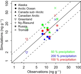
Figure 7.Same as Fig. 3, but for Exp. D with standard
precipita-tion (red symbols), 50 % precipitaprecipita-tion (green symbols), and 200 % precipitation (blue symbols). See text for details.
creases annual BC deposition by 16 % in the Arctic. This is because less precipitation removes fewer BC particles. BC lifetime in the Arctic, as determined by the BC loading and deposition, increases by 27 %. When precipitation is dou-bled, annual BC loading decreases by 14 %, while BC de-position increases by 8 %, resulting in a 23 % reduction of BC lifetime in the Arctic.
BCair is more sensitive to precipitation at Barrow, Alert,
and Zeppelin than at Denali and Summit (Fig. 8). When pre-cipitation is halved, annual BCair increases by 20–70 % at
Alert, by 10–40 % at Barrow and Zeppelin, and by 1–20 % at Denali and Summit. When precipitation is doubled, annual BCairdecreases by 20–50 % at Alert, by 10–40 % at Barrow
and Zeppelin, and by 2–20 % at Denali and Summit. Addi-tionally, BCair is more sensitive to precipitation in summer
than in winter. This is because the summer clean boundary layer in the Arctic is controlled by strong local scavenging (Garrett et al., 2010, 2011; Browse et al., 2012).
4.5 BC in snow in Greenland, Tromsø, and Canadian sub-Arctic
BCsnow is associated with much larger uncertainties over
short (hence shallower snow depth) than longer (hence larger snow depth) time periods. Because snow samples over Greenland were collected at the very surface (∼0 cm),
the computed BCsnow thus represents BC deposition only
through the duration of a day for direct comparisons. The short time duration thus largely explains the larger uncertain-ties in the estimated BCsnow. In Tromsø, observed BCsnow