Stochastic frontier analysis applied to the fisheries

(1)

UNIVERSIDADE DE LISBOA FACULDADE DE CIˆENCIAS DEPARTAMENTO DE ESTAT´ISTICA

E INVESTIGAC¸ ˜AO OPERACIONAL

STOCHASTIC FRONTIER ANALYSIS

APPLIED TO THE FISHERIES

Nuno Madeira Veiga

MESTRADO EM ESTAT´ISTICA 2011

(2)

(3)

UNIVERSIDADE DE LISBOA FACULDADE DE CIˆENCIAS DEPARTAMENTO DE ESTAT´ISTICA

E INVESTIGAC¸ ˜AO OPERACIONAL

STOCHASTIC FRONTIER ANALYSIS

APPLIED TO THE FISHERIES

Nuno Madeira Veiga

Disserta¸c˜ao orientada pela Prof. Doutora Maria Luc´ılia Carvalho e supervisionada pela Doutora Ivone Figueiredo

MESTRADO EM ESTAT´ISTICA 2011

(4)

(5)

Aknowledgments

A presente tese foi desenvolvida no ˆambito do projecto DEEPFISHMAN, FP7-KBBE-2008-1-4-02, Management and Monitoring of Deep-sea Fisheries and Stocks.

Quero agradecer...

`

A Dra. Ivone,

por ter acreditado no meu valor, pelo que me fez evoluir e aprender durante este tempo. `

A Prof. Luc´ılia,

por ter apostado em mim, pelo que me proporcionou e pelo que me transmitiu. `

A Prof. Isabel,

pelo apoio e pela ajuda para a apresenta¸c˜ao do poster. Aos meus colegas do Ipimar,

pela calorosa recep¸cão, pela fácil integra¸cão e pela inesgotável simpatia. Aos meus amigos,

por serem amigos no verdadeiro sentido da palavra. `

A minha namorada,

por todo o apoio, amor e paciˆencia que tiveste e tens para comigo e por seres a fonte da minha for¸ca.

Ao meu pai, irm˜a e cunhado,

pelo apoio incondicional ao longo destes seis anos.

`

A minha m˜ae,

por n˜ao me ter deixado desistir . . .

(6)

(7)

Abstract

In fisheries world the knowledge of the state of the exploited resource, is vital to guar-antee the conservation of the resource and the sustainability of the fishery itself. The present study is focused on the Portuguese longline deep-water fishery that targets black scabbardfish. This fish is a deep-water species and its landings have an important eco-nomical value for Portugal. The fleet that explores the species is composed by 15 vessels with a mean overall length of 17 m.

In the first part of this work Generalized Linear Model was used to standardize the Capture-per-unit-effort, so the first aim is to improve the estimate of CPUE, which is widely used as an index of stock abundance. This is done by reanalyzing the data stored at Portuguese General Directorate from fishery industry and in particularly the logbooks, which are used to record catch data as part of the fisheries regulation.

The second part focused on Technical Efficiency, which refers to the ability to mini-mize the production inputs or the ability to obtain the maximum output. In this study TE estimates were obtained through Stochastic Frontier Analysis. This methodology em-braces two science fields, Economy and Statistics, and has been the subject of studies in various areas but there are few applications to fisheries and the available ones are often studied from the economic point of view rather than a statistical one.

This work aimed to analyze the quality of the logbooks and identify the relevant factors to the CPUE estimation as the theoretical evaluation of SFA approach and the identification of the statistical differences between several models. TE of each vessel was estimated and was verify if the black scabbardfish fishery operating in Portugal mainland can be considered efficient.

Keywords:

Black scabbardfish, Catch-per-unit-effort, Generalized Linear Models, Stochastic Frontier Analysis, Technical Efficiency.

(10)

(11)

Resumo

Portugal é um pa´ıs costeiro com cerca de 1200 km de costa, fazendo da pesca uma das actividades mais importantes, económica e culturalmente. Uma das espécies mais pescadas em Portugal é o peixe-espada preto, fazendo desta espécie uma das mais estu-dadas devido ao seu impacto socioeconómico. Desde o século XVII que na Madeira, o peixe-espada preto é pescado, mas só em 1983 foi iniciada esta pesca em Portugal con-tinental, sendo Sesimbra a principal zona pesqueira. Assim sendo, foi de Sesimbra que vieram grande parte dos dados que foram usados neste trabalho.

A regula¸cão e a gestão da actividade pesqueira continuam a ser um dos maiores de-safios, sendo assim essencial a avalia¸cão do estado dos recursos explorados (neste caso o peixe-espada preto). Tal avalia¸cão é vital para procurar medidas que garantam a sus-tentabilidade do recurso e da pesca.

Um dos ´ındices de abundância mais utilizados é o CPUE (captura-por-unidade-esfor¸co), que é definido como a razão entre o total capturado e o total de esfor¸co aplicado nessa mesma captura. Apesar do seu frequente uso é sabido que o CPUE é influenciado por outros factores para além do n´ıvel de abundância. Assim, para minimizar essa influência, o CPUE é estandardizado de forma a diminuir ou até remover os eventuais factores de confusão. Para tal foram aplicados Modelos Lineares Generalizados (GLM), que não são mais do que uma generaliza¸cão dos Modelos Lineares. Essa generaliza¸cão permite que a distribui¸cão da variável resposta perten¸ca à fam´ılia exponencial (para além da Normal), e permite que a fun¸cão de liga¸cão entre a variável resposta e as variáveis explicativas seja uma fun¸cão monótona diferenciável.

Para estimar tal ´ındice, a fonte de dados é frequentemente o diário de bordo. Na União Europeia e desde a introdu¸cão de Pol´ıtica Comum das Pescas, que reúne várias medidas para garantir a sustentabilidade da pesca europeia, é obrigatório registar toda a viagem desde a partida do porto até ao desembarque. Além disso, dado que não há dados independentes da pesca, ou seja, não há estudos dirigidos para a recolha de dados através de amostragem, a estima¸cão deste tipo de ´ındices acaba por depender quase exclusiva-mente dos diários de bordo. Assim acabam por assumir uma importância vital quer na monitoriza¸cão quer na regulamenta¸cão da actividade pesqueira.

(12)

O preenchimento destes diários de bordo é feito pelos mestres das embarca¸cões no mar e é posteriormente introduzido numa base de dados pela Direçcão Geral das Pescas e da Aquicultura. Contudo há erros ou más interpreta¸cões no preenchimento dos diários de bordo que podem de alguma forma enviesar quer os resultados quer as conclusões de estudos neles baseados. Além de que os dados retirados dos diários de bordo reflectem sempre imensa variedade nas espécies capturadas além da espécie alvo. Apesar disto, os diários de bordo são a fonte de dados de vários trabalhos que visam estimar n´ıveis de abundância.

Desta forma, é necessário medir e quantificar o impacto que uma base de dados menos cuidada pode ter na qualidade e na veracidade dos trabalhos que nela se baseiam. É este objectivo que visa a primeira parte deste trabalho (chapter 2), usando os dados conti-dos nos diários de bordo da frota que opera em Sesimbra e que tem como espécie alvo o peixe-espada preto. Os factores e variáveis relevantes para a estima¸cão do CPUE também foram identificadas, assim como a respectiva influência.

Desta primeira parte do trabalho resultou uma análise extensiva e detalhada dos diários de bordo, permitindo identificar os erros e até nalguns casos corrigi-los através do conhecimento de trabalho anteriores e da comunidade pesqueira de Sesimbra. Análise essa que recorreu a várias ferramentas estat´ısticas (p.e. Análise de Clusters, Tabelas de Contingência, e Testes de Significância) e que foi suportada por análise gráfica (p.e. Scatter-plots, QQ-plots e Histogramas). Foi poss´ıvel então comparar os resultados obti-dos entre duas bases de daobti-dos, uma mais cuidada do que outra no que toca ao registo de observa¸cões. Diferen¸ca essa que foi bem vis´ıvel na percentagem de explica¸cão do modelo, onde houve um decréscimo de 20 pontos percentuais.

Inspirada nestes resultados, surgiu a ideia de aplicar outra abordagem e usar outra fonte de dados que não os diários de bordo. A sustentabilidade do recurso, para além de outros factores, passa pela utiliza¸cão eficiente de recursos de modo a garantir a renova¸cão constante do peixe para n´ıveis óptimos. Tal eficiência só pode ser atingida minimizando o desperd´ıcio dos recursos gastos durante a actividade pesqueira e maximizando o proveito socioeconómico dessa mesma actividade.

Apesar deste conhecimento geral, nem todos os produtores (neste caso embarca¸cões) são bem sucedidos em atingir n´ıveis satisfatórios de eficiência. Existem várias aborda-gens para estimar e avaliar a eficiência duma actividade económica, em particular Análise de Fronteiras Estocásticas (SFA), que combina dois campos da ciência, a Estat´ıstica e a Economia. Esta metodologia foi desenvolvida por Aigner and Schmidt [1977] e por Meeusen and van den Broeck [1977], e tem sido aplicada em vários campos e sido objecto de várias pesquisas, sendo até considerada por alguns autores como a melhor abordagem na presen¸ca da ineficiência. Dentro desta metodologia podem ser consideradas três tipos

(13)

CONTENTS ix

de eficiˆencia: T´ecnica (Technical Efficiency), Custo (Cost Efficiency) e Lucro (Profit Ef-ficiency).

Neste estudo apenas foi estimada a Eficiência Técnica que pode ser descrita como a habilidade de, dado um resultado fixo (output), minimizar a quantidade de variáveis (inputs) necessárias para obter tal resultado, ou a habilidade de maximizar o resultado obtido de um conjunto de variáveis fixas. O conceito é simples e até tem havido um crescente interesse em aplicar esta metodologia à actividade pesqueira, no entanto são poucos os trabalhos realizados sobre este tema, e os poucos que há são estudados duma perspectiva económica e não estat´ıstica. Assim este trabalho vem, de alguma forma, ten-tar preencher esse vazio realizando esta abordagem do ponto de vista estat´ıstico.

A segunda parte deste trabalho (chapter 3) tem então o propósito de avaliar esta abor-dagem teoricamente e verificar se é na prática uma ferramenta útil e de fácil aplica¸cão. Assim, dentro deste estudo, a eficiência técnica de todas as embarca¸cões que compõem a frota de peixe-espada preto de Sesimbra foram estimadas. Para tal foram recolhidos dados através de inquéritos aos envolvidos nesta actividade, sendo obtido dados relativos aos anos de 2009 e 2010.

Dos resultados foi poss´ıvel identificar diferen¸cas entre várias abordagens e modelos, avaliar a evolu¸cão da eficiência no tempo, procurando tendência e/ou sazonalidade e fi-nalmente verificar que a pesca do peixe-espada preto desenvolvida em Sesimbra pode ser considerada eficiente.

Palavras-chave:

Peixe-espada preto, Captura-por-unidade-esfor¸co, Modelos Li-neares Generalizados, Análise de Fronteiras Estocásticas, Eficiência Técnica.

(14)

(15)

Chapter 1 Introduction

On the Portuguese continental slope, in the south of ICES Division IXa, the long-line fishery targeting black scabbardfish was initiated in 1983 at fishing grounds around Sesimbra. In Madeira Island there is also a fishery targeting this species which dates back to the 17th century. At present, the fleet targeting black scabbardfish in Portuguese waters is composed by small vessels that still display artisanal features (see Figueiredo and Bordalo-Machado [2007] for detailed description).

Longline fishery is a commercial fishing technique which uses (as the term indicates) a long line, called mainline, with several branch-lines attached as Figure 1.1 shows. Fishing operations usually start at dusk and two manoeuvres generally occur: the newly baited longline gear is deployed into the sea and another longline gear, previously set in the last 24-48 hours is recovered, usually with the aid of a hauling winch. Thus the soaking time of the fishing gear in sea is more than 24h and on average 46h. The preparation of one single gear takes some time, since it can last more than half a day. According to the stakeholders, in Sesimbra to preserve and guarantee the freshness of the fish, only one fishing haul is made by trip.

At beginning, longlines had 3600-4000 hooks, however this number has been largely increased over time, since in 2004 number of hooks ranged from 4000 to 10000. Fishing activity takes place on hard bottoms along the slopes of canyons at depths normally rang-ing from 800m to 1200m; though 1450m has been reached in the last years. This fishery is also characterized by the fact that the fishing grounds are specific for each vessel, i.e. each fishing vessel around Sesimbra has a specific and unique place to fish. This fishery takes other deepwater species as a by-catch, i.e. during the fishery while attempting to catch the target fish, they unintentionally end up capturing other species, being the Portuguese dogfish and Leaf-scale gulper shark the principal species caught [Figueiredo and Gordo, 2005].

(16)

In the process of data collection, to evaluate the species abundance and the fishing impact, there has been in EU, since the introduction of the Common Fisheries Policy (CFP) in 1983, a requirement to record fish catches in a standard community format. This is done by skippers that record the activity at sea and such information is contained on the logbooks that might become an integral tool for monitoring and enforcement. In fact, since there is no independent data from the fishery, as the one commonly collected during directed surveys, the abundance index of black scabbardfish relies on information collected from the fishery itself.

Therefore this knowledge, detailed in logbooks, is vital to define fishery policies and this way to ensure a sustainable activity. Because of this importance is necessary to know, through the logbooks (and other data sources), which variables and factors are important in the performance of the fishery, being fundamental to this end, establish a correct mea-surement for that performance (CPUE) and estimate the efficiency of the vessels involved and what variables it depends.

This way in chapter 2 the quality of the logbooks data was analyzed in detail and the significant factors for the estimation of the CPUE were identified. Whereas chapter 3 aimed apply Stochastic Frontier Analysis to estimate the Technical Efficiency of the vessels involved in this fishery.

(17)

Chapter 2 CPUE study based on information

contained in logbooks

2.1 Introduction

Portugal is a coastal country with about 1200 km of coastline. Therefore the fishery have been throughout history, a present activity in the culture and in the economy of this country. This activity has become of crucial economic importance reinforcing the trade and the related arts. For any fishery the knowledge of the state of the exploited resource is vital for the evaluation of the fishing impact, as well as, for the proposal of management rules that guarantee the sustainability of the resource and consequently of the fishery.

These were the motivations for this study focused on the black scabbardfish fishery, which is the one of the most important fisheries ongoing in Portugal.

As mentioned above the data source used was the logbook. There are however errors or misinterpretations on how to fulfil these logbooks that might hinder its use and pur-poses related to stock status evaluation. Moreover data in logbooks sampled directly in the field, often reflect the presence of a variety of other species or habitats targeted by the fishermen, even within a single fishing trip. Consequently, some of the records in data may not be relevant to evaluate the stock status of only one target species. Despite this fact, the data contained in logbooks have been used in several working papers to calculate measures of effort like Catch-per-unit-effort (CPUE).

CPUE is defined as the total catch divided by the total effort spent to obtain that catch and is commonly used as an abundance index over time. That effort, in this case fishing effort, may be measured by several variables (e.g. number of vessels, soaking time and number of hooks) and in the recent years considerable energy has been applied by researchers to develop reliable measures of fishing effort. Despite the frequent use, it is

(18)

known that CPUE is influenced by many factors other than abundance. Thus to mini-mize that unwanted influence CPUE is standardized, through this process the effect of confounding factors is reduced or even removed [Maunder and Punt, 2004].

In statistic the fitted models have two main objectives, estimation of the model pa-rameters and the prediction of the study variable values. In CPUE standardization the appropriate modeling strategy is to build an estimation model, rather than a predictive. To do so, it was used the Generalized Linear Model (GLM), which is recognized as a valuable tool for the analysis of fisheries data [Maunder and Punt, 2004].

Linear Models (also known as Regression Model) are used when it is assumed that the study variable (known as the response or dependent variable) has a linear relationship (Y = βX + ε) with other variables (denoted as independent or explanatory variables) and the distribution of the response variable is assumed to be Normal. However these assumptions are rarely encountered in the real world and to overcome these restrictions the GLM, which are a flexible form of linear models, were built.

The GLM generalizes Linear Models by allowing two new possibilities: the distribu-tion of the response variable may come from any member of the exponential family other than the Normal (e.g. Gamma, Poisson, Binomial...) and the link function (the link between response variable and the independent variables) may come from any monotonic differentiable function (e.g. inverse function, log function...) as detailed in McCullagh and Nelder [1989]. Despite the limitations still imposed, the GLM have been acquiring an increasingly important role in statistical analysis.

Summarizing, the first part of this work critically analyzes the data contained in the logbooks from the Portuguese fleet operating with longline in Portugal mainland (Sesim-bra). The quality and mainly the reliability of the logbooks and the consequences of the absence of carefully collected data, were assessed and analyzed in detail. Finally after being found the best way to set the CPUE, the factors relevant for the estimation of the CPUE of black scabbardfish fishery were identified as well as their influence on the CPUE.

2.2 Materials and Methods

2.2.1 Data and Variables

Two different sets of logbook data were available: one covering the period from 2000 to 2005 and the second one covering the period from 2000 to 2008.

The first data set (covering five years) was, prior to this work, reviewed in detail. This set included trip data on the following variables: vessel identification code (ID); fishing gear; port and date of departure; port and date of arrival; number of fishing hauls

(19)

2.2 Materials and Methods 5

(NHAUL); soaking time (ST); ICES rectangle where fishing haul took place (ERECTAN); ICES subarea; caught species (SP); catch weight by species in kilogram (CATCH) and number of hooks used in each fishing haul (HOOKS). This last variable was obtained by detailed revision, so it was absent in the second data set.

This set had 9330 trips and since each trip had multiple records of different species, they produce a total of 32136 records from 31 vessels. This means that, for the variables SP and CATCH there were altogether 32136 observations (records) and for other variables, since they are unique for the each trip, there were 9330 observations (trips).

The data set was then restricted to trips in which deep-water longline (LLS) was used. This restriction was essential since the studied fishery only uses such fishing gear. The restriction resulted in 7095 trips with 24235 records (around 75% of initial number of records) and 28 vessels. Among these, positive catches of black scabbardfish were only reported for 22 in a total of 5507 records, which in this case coincided with the total number of trips, because a single species was being considered (about 60% of initial number of trips). However information on the number of hooks used was available only for 2514 trips (unfortunately, the fishermen do not usually fill this field in logbooks).

The second set included the data stored at the Portuguese General Directorate for Fisheries and Aquaculture (DGPA) database. This information covered data on a trip basis of all the variables mentioned before, except the HOOKS. In total the data set had 14319 trips with 77483 records (representing 102 vessels) but only 8764 trips with positive catches of black scabbardfish where LLS was employed (around 61% of initial number of trips).

Additionally information on the daily landings of vessels that landed in the Portuguese ports were also available. However in this database each record contained only information about the ID, port and date of arrival, fishing gear, SP and weight and selling price of the fish landed. In this case the number of records regarding positive catches of black scabbardfish was 52734, however due to multiple landings (in different ports) this number was actually 52051 (see Table 2.1 for summarized information).

Table 2.1: Summary of Database about missing variables (x means present)

Database _Period _{No of Records NHAUL} _{ST HOOKS ERECTAN}

1st _{Data set} _2000-2005 ₅₅₀₇ _x _x _x _x

2nd _{Data set} _2000-2008 ₈₇₆₄ _x _x _x

(20)

2.2.2 Exploratory Data Analysis

As previously stated, the analysis of both data sets was based on data restricted to the trips where the longline was the fishing gear used (LLS) and the quantity caught of black scabbardfish (BSF) was positive. Posteriorly three extra variables were considered. The first one called TOTAL was added to the two data sets and corresponds to the total weight caught per trip, i.e. the sum of the weight of all species caught in each trip.

As mentioned before the main by-catch species of the Portuguese black scabbardfish fishery are the sharks Portuguese Dogfish - CYO and Leafscale Gulper Shark - GUQ. Therefore the relationships between the CYO and GUQ catch values and the BSF catch values were evaluated. To do so, catch values of CYO and GUQ were considered as well as two new variables: i) PERC which corresponded to the percentage of BSF in the TOTAL; ii) RATIO which gives the percentage of BSF catches in the sum of catches of BSF, GUQ and CYO, i.e. CATCH of BSF /(CATCH of BSF + CATCH of CYO + CATCH of GUQ). These two last variables were taking into consideration due to the fact that the weight of the two deepwater sharks are very different from the weight of BSF.

Additionally there was also information on vessels technical characteristics, namely length-over-all (XCOMP), gross registered tonnage (XTAB) and power of the engine in horse power (XPOW). These features summarizes the main characteristics of the vessels and are invariant throughout time according to stakeholders.

1st _{Data set}

Data contained in the 1st _{set was analyzed to identify possible discrepancies on each}

variable values, particularly on soaking time (ST), number of hauls (NHAUL) and number of hooks (HOOKS). The analysis included i) graphical analysis (e.g. boxplots, histograms and scatter plots) and ii) confronting the data with the knowledge on the exploitation regime of the BSF fishery. The graphical analysis was made by plotting the CATCH of BSF versus each of the these three variables. To clarify some of the identified dis-crepancies, inquiries to stakeholders and to DGPA authorities responsible for database maintenance were made.

The analysis continued by defining criteria to distinguish vessels with a regular activ-ity targeting BSF from those for which the capture of BSF could be considered sporadic. Such restriction was critical to eliminate confounding vessels and consequently confound-ing observations in the data. This analysis was based on comparconfound-ing the cumulative sum of CATCH of BSF (per vessel) with the cumulative sum of total catch (of all species) and in the estimation of the proportion of BSF in that sum.

(21)

con-2.2 Materials and Methods 7

stant activity targeting BSF (15 vessels with 5440 records). To evaluate the relationship between CATCH and the variables ST, NHAUL and HOOKS, Pearson’s correlation co-efficients were estimated sustained by a graphical analysis. To exclude the potential confounding effect of the factor vessel, similar analysis was applied separately to a subset of three vessels selected using three criteria: i) they had the longest records; ii) they did not have problematic observations in variables HOOKS and ST; and iii) together they represented the majority of total records (51%).

The relationship between the two main by-catch species (GUQ and CYO) and the tar-get species (BSF) was also evaluated using the two variables previously described (PERC and RATIO). This analysis was done by estimating the Pearson’s correlation coefficient between PERC (same for RATIO) and CATCH of CYO, CATCH of GUQ and CATCH of CYOGUQ (i.e. CATCH of CYO + CATCH of GUQ).

The relation between the geographical location of fishing grounds (ERECTAN) and the catch of BSF was also investigated. To this end, since ERECTAN is a categorical variable, contingency tables were used to test the independence between the two variables. In this analysis two spatially adjacent rectangles 05E1 and 05E0 were joined, because they are next to each other and 05E1 is obviously an error since it is in the mainland (Fig. 2.1). The total catch of BSF (in kg) was discretized into the following levels: 0 – 500; 500 – 1000; 1000 – 1500; 1500 – 2000; 2000 – 2500; > 2500, which were defined taking into account the minimum and maximum catches and to prevent further problems in the application of independence tests. Particularly, the Pearson chi-square independency test which requires that all expected frequencies have to be at least one and no more than 20% of the expected frequencies can be less than 5 [Zar, 1996].

(22)

2nd _{Data set}

Through a crude analysis it was verified that the second data set contained a high number of errors, as for example: i) trips with more than 10 fishing hauls (NHAUL), such situation is impossible due to the duration of a fishing operation, when compared with the duration of a fishing trip; ii) more than 30 times of the median value of black scabbardfish caught per trip (CATCH of BSF), which is about 1 ton; iii) different soaking times (ST) assigned for different species caught in the same haul and in the same trip and iv) in some cases ST was swapped with the NHAUL (e.g. in the same trip, 12 hauls with 1 hour of soaking time). These cases are just examples of the complexity and type of errors that were present in a careless database. The procedure for the inspection and correction of data was the same applied for the 1st _{data set, however the final result of}

this correction was not so effective and efficient due to the data dimension and due to the long time that was required for such correction.

Since this data set contained a lot of conflicting and less reliable observations, a cross-checking was performed by comparing the BSF catches values recorded in the DGPA database (from hereon denoted as LBSF) with the BSF catches values recorded in the logbooks (2nd _{set and from hereon denoted as CBSF). Trips with extremely high}

discrep-ancies were excluded from the database.

The procedure applied to this data set was similar to the one applied to the 1st set, either in the treatment of the variables related to the by-catch species as well as in the selection of vessels and statistical rectangles (ERECTAN).

2.2.3 CPUE standardization using Generalized Linear Model

Standardization of commercial catch and effort data is important in fisheries where standardized abundance indices based on fishery-dependent data are a fundamental input to stock assessments [Bishop, 2006]. In the standardization of the CPUE through GLM, the variables to include in the model should be selected if there is an a priori reason to suppose that they may influence catchability. However this selection must be careful, because the inclusion of explanatory variables that are correlated should be avoided. To avoid this problem, estimation of correlation measures and corresponding graphical analysis were performed between some of the explanatory variables.

In GLM adjustment different combinations of explanatory variables were used and several output models were tested to understand the relationship between the CATCH of BSF (response variable) and the others variables. Because the 1st _{set contained more}

(23)

contribute more to explain the CATCH of BSF and to select the variables to enter in the model adjustment of the 2nd _{set. The GLM can be expressed through the following}

expressions:

The response variable Y has a distribution that comes from a member of exponential

family, with E(YYY ) = µµµ and constant variance σ2_;

The explanatory variables xxx1, ..., xxxp produce a linear predictor ηηη =

Pp

1xxxjβj, with

the βββ parameters to be estimated;

The link function g between the µµµ and ηηη may come from any monotonic differentiable

function ηi = g(µi), i = 1, . . . , n individual.

Several GLMs were adjusted to the final subset of data using a stepwise procedure and this procedure can be summarized in the following steps:

Step 1 - Selection of the distribution (under exponential family) that best fits to

the response variable. Graphical analysis was performed and the distributions were adjusted via the maximum likelihood method;

Step 2 - Selection of the variables to enter in the model. Maunder and Punt [2004]

suggest to always include in the model the factor year. In this case, since the tempo-ral aspect is the major goal of the abundance analysis and given that both the year as the quarter were available, these two variables (YEAR and QUARTER) were always included in the models. The following explanatory variables were also con-sidered: HOOKS, ERECTAN, XCOMP, XTAB, XPOW, PERCCYOGUG (which represented the percentage of Leafscale Gulper Shark and Portuguese Dogfish on the total weight caught, i.e. (CYO + GUQ) / TOTAL). The absolute values of CATCH of CYO and GUQ were not used because, as mentioned before, their weights are very different in scale from the weight of BSF. In the construction of this last variable the missing values of CATCH of CYO and GUQ were replaced by zero;

Step 3 - Choice of a link function compatible with the distribution of the proposed

error for the data. This choice must be based on a set of considerations made a priori [Turkman and Silva, 2000]. For the Gamma distribution the logarithmic link function is recommended, whereas the identity link is recommended for the Lognormal distribution;

Step 4 - Selection of the best model adopting a parsimonious criterion (model with

the smallest number of explanatory variables but a high fit to the data). The de-viance function and the generalized Pearson χ2 _{statistic were estimated to assess}

(24)

the models quality of adjustment. Both statistics follow an approximate χ2

distri-bution with n - p degrees of freedom, where n is the sample size and p the number of parameters. However asymptotic results may not be specially relevant even for large samples [McCullagh and Nelder, 1989]. The information criterion of Akaike, denoted as AIC and based on the log-likelihood function, was also used. The lower the value of AIC is, the better is the models adjustment. AIC is a flexible likelihood-based approach, which is commonly used in model selection, having the advantage of allowing the comparison of non-nested models. However has the disadvantage of usually choose a complex model (with more variables) instead of a simpler one. To measure the goodness of fit the adjusted coefficient of determination, which corre-sponds to the ratio of the residual deviance with the null deviance and its respective degrees of freedom (ρ2_{), was also used [Turkman and Silva, 2000];}

Step 5 - Model checking by residual graphical analysis. Plots of residuals against

different functions of the fitted values, as well as residuals against an explanatory variable in the linear predictor were performed (as suggested by McCullagh and Nelder [1989]). Three residuals were considered and in the following expressions the Turkman and Silva [2000] notation was used:

Standardized Pearson Residual:

RP_i = q yi− ˆµi \

var(Yi)(1 − hii)

, (2.1)

where hiiare the diagonal elements of the ’hat’ matrix, which describes the influence

of each observed value on each fitted value. Anscombe Residual: R_iA= qA(yi) − A(ˆµi) \ var(Yi)A′(ˆµi) , A(x) = Z 1 V1/3_(x)dx, (2.2)

where V (x) is the variance function. Standardized Deviance Residual:

R_iD = sign(yi− ˆµi) √ di q ˆ φ(1 − hii) , (2.3)

(25)

where ˆφ is the dispersion parameter estimate and di is the contribution of the i − th

observation for the deviation of the GLM.

Both the Pearson and Anscombe residuals are expected to have a distribution close to Normal, however generally the distribution of the Pearson residuals is very asym-metric for non Normal models. In the case of Deviance residuals, is recommended by McCullagh and Nelder [1989] to plot against fitted values or transformed fit-ted values (for each distribution family there is one specific transformation). It is expected that the distribution of these residuals occurs around zero with constant variance.

Step 6 - Identification of conflicting observations which can be categorized in three

different ways: leverage, influence and consistency.

An indicator of the influence of the i − th observation can be calculated by the difference ˆβˆβˆβ(i)− ˆβˆβˆβ, where ˆβˆβˆβ(i) denotes the estimates without the extreme point i and

ˆ

βˆβˆβ with it. If this difference is high, the observation i can be considered influential and its exclusion can produce significantly changes in the parameters estimates.

An isolated point of high leverage may have a value of hii such that nh_pii > 2

[Mc-Cullagh and Nelder, 1989], where hii are the diagonal elements of the ’hat’ matrix

and p is the trace of the ’hat’ matrix (i.e. the sum of diagonal elements). The ’hat’ matrix describes the influence of each observed value on each fitted value (i.e. the influence of YYY in µµµ), therefore the leverage measures the effect of the observation in the matching fitted value.

For the last kind of conflicting observation, an inconsistency observation can be considered as an outlier. Williams [1987] suggests plotting the likelihood residuals (detailed below) against i or hii to study the consistency of observation i.

RL_i = sign(yi− ˆµi)

q

(1 − hii)(RDi )2+ hii(RPi )2. (2.4)

Note that RD

i and RPi are respectively the Deviance and Pearson residuals detailed

(26)

2.3 Results

2.3.1 Exploratory data analysis

The knowledge already available for the longline fishery operation, allowed to identify the major inconsistencies both in the 1st_{and the 2}nd _{data sets. After a crude analysis the}

most obvious inconsistencies corresponded to null soaking time (ST) and to more than 10 fishing hauls per trip. Other discrepancies consisted on dates of arrival earlier than date of departure, however fortunately some of the discrepancies found were later corrected by logbooks scrutiny and through enquiries to the fishermen. As mentioned previously, the exploratory data analysis began to be made to the 1st _set.

1st _{Data set}

In this set the variables HOOKS was the first to be analyzed. The histogram of the number of hooks (HOOKS) used per trip, showed the existence of a group of trips in which the number of hooks was much smaller than the number commonly used. Note that despite this fact, the quantity of fish caught was similar in both groups (as can be seen in the scatter plot of Fig. 2.2). As a result it was considered only the trips in which it was used more than 3000 hooks (taking into consideration the knowledge of the stakeholders and the previous works on this matter).

Histogram of HOOKS HOOKS Density 2000 4000 6000 8000 0e+00 2e−04 4e−04 6e−04 8e−04 1e−03 2000 4000 6000 8000 Boxplot of HOOKS 2000 4000 6000 8000 0 1000 2000 3000 4000 5000 HOOKS vs BSF HOOKS BSF

Figure 2.2: Histogram, Boxplot and Scatter plot of CATCH of BSF versus HOOKS.

As mentioned previously, before analyzing the other variables, it is important to dis-tinguish between vessels with a regular activity targeting BSF and those for which the capture of BSF can be considered sporadic. There was no value set a priori, but this

(27)

2.3 Results 13

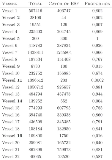
selection was based on two variables: sum of CATCH of BSF of each vessel (Tab. 2.2) and proportion of BSF catch values on the total catch considering the whole time period (i.e. sum of CATCH of BSF / sum of TOTAL, for each vessel and for all trips made). In this table vessels numbered as 2, 3, 9, 11, 14, and 19 (all in bold) had proportions of CATCH of BSF lower than 1.6%, which is very low compared with the remaining vessels. The vessel 5 (in bold), despite having 100% of CATCH of BSF only landed 300 kg of BSF, which was very low when compared with other vessels. Based on these results the subset of 15 vessels was considered for the remaining analysis resulting in a loss of only 0.5% of observations.

Table 2.2: Proportion of CATCH of BSF in the TOTAL catch from 2000 to 2005.

Vessel Total Catch of_BSF Proportion

Vessel 1 507416 406747 0,802 Vessel 2 ₂₈₁₀₆ ₄₄ _0,002 Vessel 3 ₁₉₅₅₁ ₁₂₉ _0,007 Vessel 4 235603 204745 0,869 Vessel 5 ₃₀₀ ₃₀₀ ₁ Vessel 6 418782 387834 0,926 Vessel 7 1438811 1245804 0,866 Vessel 8 197534 151408 0,767 Vessel 9 ₆₇₃₀ ₁₀₀ _0,015 Vessel 10 232752 156885 0,674 Vessel 11 _1396512 ₂₃₃ _0,0002 Vessel 12 1050712 925657 0,881 Vessel 13 484794 457478 0,944 Vessel 14 ₁₃₉₂₅₂ ₅₅₂ _0,004 Vessel 15 774293 607795 0,785 Vessel 16 394740 339338 0,860 Vessel 17 436599 345385 0,791 Vessel 18 158184 132950 0,841 Vessel 19 ₁₀₉₈₀₀ ₁₇₅₀ _0,016 Vessel 20 259081 165732 0,640 Vessel 21 862399 759973 0,881 Vessel 22 40065 23520 0,587

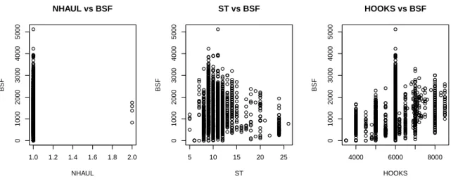
To evaluate the relation between CATCH of BSF and the variables ST, NHAUL and HOOKS (potential measures of effort), Pearson’s correlation coefficients were estimated (Tab. 2.3) sustained by a graphical analysis. All the correlations obtained were relatively low even when different combinations of the three variables were considered (e.g. NHAUL × ST).

Beginning with the evaluation of the variable NHAUL, for most of the fishing trips only one fishing haul was performed, remaining only four trips in which two hauls were

(28)

recorded (Fig. 2.3), and yet when two fishing hauls were performed the catch value of BSF did not increased. This lack of variability did not allow to consider the number of hauls as a variable, so NHAUL was not taken into account in the remaining analysis. Notice that this variable was the only one, among the three variables, for which the independency hypothesis with CATCH of BSF was not rejected, with p-value ≈ 0.8.

As for the variable ST, this had a quite large range, however using the knowledge available on fishery, ST < 24h are almost impossible since the fishing gear stays at the fishing ground at least 24h. Thus the values of ST lower than 24h were considered as errors, such errors could probably resulted from a generalized misinterpretation of the variable by fishermen. Instead of including the soaking time they introduced the travel time to the fishing ground. Thus this variable may loose its utility in this study, however through the Pearson’s independency test, the independency was rejected with p-value ≈ 6e-06.

In the analysis of the ST it was verified, through a graphical analysis, the existence of two main groups of records (ST < 24h and ST ≥ 24h). However in Table 2.4 the trips with ST ≥ 24h were only registered in 107 trips and it was not possible to identify a vessel or a group of vessels that systematically reported ST ≥ 24h. This way this variable was not taken into account for the remaining analysis, since ST did not correspond to the soaking time of fishing haul in sea.

The analysis of HOOKS showed that, among the three variables, this one was the most significant (null hypothesis rejected with p-value ≈ 0), in sense that it had the highest value on Pearson’s coefficient (Tab. 2.3) and the plot showed a slight positive trend (Fig. 2.3). Despite these facts, the variable did not achieve high indices of linear correlation with CATCH of BSF (only 0.31).

Table 2.3: Pearson’s coefficient between CATCH of BSF and the variables HOOKS, ST and NHAUL.

Pearson’s Correlation HOOKS ST NHAUL

Catch of BSF 0.31 -0.09 0.005

Next it was considered the subset of three vessels (the choice was based on three criteria detailed before) and it was considered only the variables HOOKS and ST (Tab. 2.5). For this subset the Pearson’s correlation coefficient, between CATCH of BSF and HOOKS, decreased when compared with the global value. For ST the correlation coeffi-cient increased for Vessel 3, but the improvement was not significant nor regular among the vessels (with positive and negative values). Therefore since neither of the variables showed significant differences in correlation with CATCH of BSF, the 15 vessels were again considered.

(29)

2.3 Results 15 1.0 1.2 1.4 1.6 1.8 2.0 0 1000 2000 3000 4000 5000 NHAUL vs BSF NHAUL BSF 5 10 15 20 25 0 1000 2000 3000 4000 5000 ST vs BSF ST BSF 4000 6000 8000 0 1000 2000 3000 4000 5000 HOOKS vs BSF HOOKS BSF

Figure 2.3: Plot of CATCH of BSF against the variables: NHAUL, ST and HOOKS.

Table 2.4: The total number of records and the number of records with at least 24h of ST per Vessel. Vessel No of records No of records with ST ≥ 24h

Vessel 1 510 3 Vessel 2 299 0 Vessel 3 682 72 Vessel 4 693 0 Vessel 5 120 0 Vessel 6 246 1 Vessel 7 468 0 Vessel 8 316 0 Vessel 9 695 0 Vessel 10 265 30 Vessel 11 270 0 Vessel 12 90 0 Vessel 13 328 1 Vessel 14 426 0 Vessel 15 31 0

Table 2.5: Pearson’s coefficient between CATCH of BSF and HOOKS / ST for a subset of three vessels.

Vessel _{/ Variable} _HOOKS _ST

Vessel 1 0.14 -0.16

Vessel 2 -0.08 -0.09

Vessel 3 0.19 0.09

To study the correlation between catches of BSF (represented by RATIO and PERC) and the main by-catch species (CYO and GUQ), the estimates of Pearson’s correlation coefficient were estimated and are presented in Table 2.6. All the estimates were signif-icant (p-value ≪ 0.01 for all estimates) and greater than 0.5 (in modulus). Therefore

(30)

catch levels of sharks affects the catch levels of BSF, particularly catches of CYO as can be observed in the variable RATIO. This analysis supported the fact that the catches of the two deep-water sharks have significant negative correlation with CATCH of BSF.

Finally regarding the ERECTAN variable, the null hypothesis of independence be-tween ERECTAN and the catches of BSF was rejected (X2 _{≈ 1035 and p − value ≈0).}

Table 2.6: Pearson’s coefficient between PERC/RATIO and CATCH of: CYO; GUQ and CYO+GUQ.

Pearson’s Coefficient CATCH of CYO CATCH of GUQ CATCH of CYOGUQ

PERC -0.53 -0.52 -0.68

RATIO -0.75 -0.65 -0.70

For the adjustment of the GLM model a new factor associated with the vessels char-acteristics was created. It is important to note that there are different vessels, both in characteristics and in the total catch of BSF, therefore it is necessary to quantify the weight and the significance of these differences in characteristics on the total catch of BSF.

Considering each vessel as a factor is clearly an exaggeration, when it comes to degrees of freedom and because there are vessels that are similar in their main features. Therefore the vessels were grouped by the variables that best describes them: XTAB; XPOW and XCOMP. The levels of these factors correspond to the groups identified after a cluster analysis was applied to the matrix of vessel’s characteristics. As those characteristics were found to be highly correlated (Tab. 2.7), one of them should be enough to characterize the vessels, consequently four different cases were considered and groups of vessels were defined based on the results from the following cluster analysis (Fig. 2.4):

In the first case all the three vessels characteristics were considered at once. Due

to the high correlation between them, it was used for clustering the Mahalanobis distance, which is the most appropriate distance function for these cases. This way five clusters were identified with the complete-linkage approach, which resulted in the assembly of a new discrete variable: CLUSTER-ALL with five levels.

Then it was considered a feature at a time. For the cluster analysis on XTAB,

the results were added as CLUSTER-XTAB, and for the variables XCOMP and XPOW the procedure was similar. In all three analyzes the Euclidean distance and the average-linkage approach were used. For all approaches four groups were identified.

(31)

2.3 Results 17

Table 2.7: Pearson’s correlation coefficient between vessels characteristics.

Variables XTAB XCOMP

XCOMP 0.91

XPOW 0.93 0.85

Figure 2.4: Dendrogram for all characteristics (left above), for XCOMP (right above), for XTAB (left below) and for XPOW (right below).

(32)

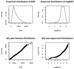
Finally the empirical distribution of CATCH of BSF was analyzed through a graphical analysis. In Figure 2.5 it appears that the variable had a positively skewed distribution (Lognormal and Gamma characteristics) and the same figure suggests the Gamma as the distribution that best fits to the data instead of the Lognormal (by the QQ-plot). Despite this fact, both distributions were later considered in the models adjustment.

0 2000 4000 0e+00 4e−04 Empirical distribution of BSF BSF Density 2 4 6 8 0.0 0.2 0.4

Empirical distribution of log(BSF)

log(BSF) Density 0 1000 3000 5000 0 2000 4000

QQ−plot Gamma Distribution

BSF Gamma 2 3 4 5 6 7 8 5 6 7 8 9

QQ−plot lognormal Distribution

log(BSF)

Lognor

mal

Figure 2.5: Graphical analysis of CATCH of BSF (left) and logarithm of CATCH of BSF (right).

2nd _{Data set}

This set contained much more errors than the first one, therefore the catch data on black scabbardfish reported at the logbooks (from hereon denoted as CBSF) was compared with the corresponding data from daily landings (from hereon denoted as LBSF). The analysis of their empirical distributions (Fig. 2.6) clearly indicated the existence, in the former, of extreme values, while the distribution of the LBSF seems to be much more in agreement with the empirical distribution observed for the 1st _{data set (Fig. 2.5).}

The corresponding difference between BSF catches registered in logbooks and daily landings was further assessed by computing the linear regression between them (Fig. 2.7). Although a close agreement was expected, high discrepancies were observed (Pearson’s correlation coefficient around 0.65). To trim the data the 99% quantile of the absolute differences between CBSF and LBSF was determined and all the observations which exceeded that quantile were removed from the 2nd _{set, excluding this way the higher}

differences between the two data sets. Figure 2.8 plots the empirical distribution of the new restricted data set which become quite similar and the variability of points around the regression line is much lower. Pearson’s coefficient correlation was higher than 0.95, which indicates a strong linear relation between them.

(33)

2.3 Results 19

Note however that the unmatched observations, because of discrepancies in dates, were not taken into account in this procedure. Therefore it was not possible to calculate the differences for all trips recorded in 2nd _{set, this way conflicting observations still remained}

in this set. After a detailed analysis of these observations, it was decided to remove the CBSF above the 99.5% quantile and below the 0.5% quantile.

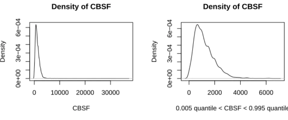
Summarizing, were applied two criteria, the first one excluded the higher discrepancies between CBSF and LBSF, and the second one removed the extreme values of CBSF. At the end, comparing the two empirical densities, the improvement is clearly visible and after these restrictions 78 vessels remained in the data set (Fig. 2.9).

0 10000 20000 30000 0e+00 6e−04 Empirical Distribution of CBSF BSF − Logbooks Density 0 2000 4000 6000 0e+00 4e−04 Empirical Distribution of LBSF BSF − Landings Density

Figure 2.6: Empirical Distribution of BSF from logbooks (left) and from daily landings (right).

0 1000 2000 3000 4000 5000 6000 7000 0 5000 15000 25000 35000 CBSF vs LBSF BSF from Landings CBSF from Logbooks

Figure 2.7: Catch of BSF from logbooks plotted against Catch of BSF from landings records.

The criteria adopted for the 1st_{data set, to differentiate vessels with a regular activity}

targeting BSF, was also applied to the 2nd _{data set. However an additional criterium}

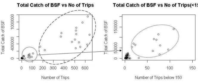
was included, since this set had a higher number of vessels. This way, the total number of trips was also used to avoid vessels with a very short time activity. To identify these vessels, for each vessel the number of trips was plotted against total CBSF (Fig. 2.10).

(34)

In the left plot it was easily identified 16 vessels, based on catches values and number of trips (inside the superior ellipse). However on the right side (which is a zooming of the left side of the figure) the selection becomes more difficult, because the number of trips and the catches values are lower. Nevertheless 11 vessels were distinguished in the dashed ellipse, which started the activity recently. Applying these criteria only 27 vessels from 78 vessels remained in the data, although this reduction just reflects a decrease of about 2.5% of number of observations (trips) and a loss of 3% of total of CBSF (sum of catch of BSF for all vessels).

0 2000 4000 6000 8000 0e+00 4e−04 Empirical Distribution of CBSF BSF − Logbooks Density 0 2000 4000 6000 0e+00 4e−04 Empirical Distribution of LBSF BSF − landings Density

Figure 2.8: Empirical Distribution of BSF from logbooks (left) and from landings records (right), using the observations with differences below 99% quantile.

0 10000 20000 30000 0e+00 3e−04 6e−04 Density of CBSF CBSF Density 0 2000 4000 6000 0e+00 3e−04 6e−04 Density of CBSF 0.005 quantile < CBSF < 0.995 quantile Density

Figure 2.9: Density of all observations and observations between 0.5% and 99.5% quantiles of CBSF.

Although the categorical variable ERECTAN was also available for the 2nd _{set, the}

level of detail was much lower than in the 1st_{set. In fact there were about 16% of records}

under the category IX, which encompass all the ERECTAN commonly frequented by the vessels and which results in an undoubtedly great loss of information, even further in such an important variable. This way, after this loss only 22 vessels were considered for the application of the GLM.

(35)

2.3 Results 21

Figure 2.10: Total catch of BSF versus number of trips (left) and the same plot zoom in (right).

2.3.2 Generalized Linear Model

1st _{Data set}

The 1st _{set is a subset of the 2}nd _{set, that was fully scrutinized in a previous work.}

So the GLM procedure was used first on this set as a way to identify the most relevant explanatory variables. In the model the response variable was CATCH of BSF (not be confounded with CBSF from 2nd _{set). In this method was also considered the factors}

YEAR and QUARTER, the interaction between them, the factor ERECTAN, the vari-ables HOOKS and PERCCYOGUQ and finally the group index levels identified on cluster analysis (CLUSTER). For detailed information about the models applied in this section see Annex 1.

The adjustment of the GLM was done through a stepwise procedure; which select the best model by AIC criterion (minimum), which tends to choose complex models with many variables. Several explanatory variables were essayed and the adequacy of the fit was evaluate based on the estimated generalized Pearson statistic and on the Deviance statistic. The p-value in both statistics was always 1, so the selected model was never rejected and Table 2.8 summarizes the results for all models tested for this data set.

Information criterion (AIC) should not be compared across different data sets, thus the models used for this set should all have the same response variable. Therefore it was not possible to compare the models with Gamma distribution with model 6, which uses the Lognormal distribution. However a substantial advantage in using information-theoretic criteria is that they are valid for nonnested models, so it was possible to compare all models with Gamma distribution since they have the same data set.

(36)

Using the Gamma distribution the best model was the number 2, because it had the lowest AIC and dispersion parameter, and the highest ρ2_{. In this model the variable}

HOOKS, which is missing from the 2nd _{data set, was included. But despite this, the}

model 5 (forcibly without HOOKS) showed that in fact the HOOKS was not so influen-tial, because the values of dispersion parameter and the ρ2 _{remained the same and the}

increase in AIC is very slight.

With Lognormal distribution, model 6 presented the highest ρ2 _{(0.62) among all}

mod-els (including the Gamma modmod-els) but this was not greatly different from the one obtained in model 2 (0.61). Since the two models came from different distributions and the ρ2 _were

identical, the comparison relied on the dispersion parameter; which showed that model 6 (0.184) deviates much more than model 2 (0.115). This is a strong indicator of the difference in goodness of fit.

Table 2.8: Resume of GLMs applied for 1st

data set.

Model 1 Model 2 Model 3 Model 4 Model 5 Model 6

Distribution Family Gamma Gamma Gamma Gamma Gamma Lognormal

Link Function Log Log Log Log Log Identity

Null Deviance 423.69 423.69 423.69 423.69 423.69 538.51 Residual Deviance 174.91 161.36 170.00 166.99 163.06 202.40 ρ2 _0.58 _0.61 _0.59 _0.60 _0.61 _0.62 Dispersion Parameter φ 0.131 0.115 0.126 0.123 0.117 0.184 AIC 16645 16554 16612 16594 16564 1291.7 Selected Variables: YEAR X X X X X X QUARTER X X X X X YEAR × QUARTER ERECTAN X X X X X X HOOKS X X X X PERCCYOGUQ X X X X X X CLUSTER X X X X X X

The residual analysis of models 2 and 6 (Fig. 2.11) presented a better fit for model 2 in relation to the hypothesis of normality of the residuals (mean around zero and constant variance). Two normality test were applied, the Lilliefors (test 1) and the Pearson test (test 2). For model 2, the normality hypothesis was not rejected (p-value ≈ 0.1 for test 1 and p-value ≈ 0.5 for test 2), whereas for model 6 the both tests rejected it with p-value ≈ 0. Thus according to the normality test, model 2 gave a better fit than the model 6.

Standardized deviance residuals were plotted against fitted values for the two models. McCullagh and Nelder [1989] said that if the data are extensive, which happened in this case, no analysis can be considered complete without this plot. The null pattern of this

(37)

2.3 Results 23

plot is a distribution of residuals with zero mean and constant range, i.e. no trend, which is verified in Figure 2.12.

Standard Pearson Residuals

Standard Pearson Residuals

Density −1.0 −0.5 0.0 0.5 1.0 0.0 0.4 0.8 −3 −1 0 1 2 3 −1.0 0.0 1.0

QQ−Plot Normal Distribution

Standard Pearson Residuals

Sample Quantiles Pearson Residuals Pearson Residuals Density −4 −3 −2 −1 0 1 0.0 0.4 0.8 −3 −1 0 1 2 3 −3 −2 −1 0 1

Pearson Residuals

Sample Quantiles

Figure 2.11: Histogram of Pearson’s Residuals (left), QQ-plot of Pearson’s Residuals (right) from Model 2 (above) and from Model 5 (below).

0 1000 3000 5000 −8 −6 −4 −2 0

Standard Deviance Residuals vs Fitted Values

Fitted Values from Model 2

Standard De viance Residuals 5 6 7 8 −8 −6 −4 −2 0

Standard Deviance Residuals vs Fitted Values

Fitted Values from Model 6

Standard De

viance Residuals

Figure 2.12: Standard Deviance Residuals plotted against Fitted Values from Model 2 (left) and from Model 6 (right).

The residuals were also plotted against the explanatory variable PERCCYOGUQ for both models 2 and 6 (Fig. 2.13). No trend was observed in the linear predictor for both models, which once again was a good indicator [McCullagh and Nelder, 1989], since the residuals are suppose to be uncorrelated with explanatory variables. Note nevertheless greater dispersion on the residuals from model 6.

(38)

0 20 40 60 80 100 −4 −3 −2 −1 0 1 PERCCYOGUQ vs Residuals PERCCYOGUQ

Residuals from Model 2

0 20 40 60 80 100 −4 −3 −2 −1 0 1 PERCCYOGUQ vs Residuals PERCCYOGUQ

Residuals from Model 6

Figure 2.13: Deviance Residuals plotted against PERCCYOGUQ from Model 2 (left) and from Model 6 (right).

Therefore, according to all the goodness of fit indices (AIC, dispersion parameter and ρ2_{), considering the residual graphical analysis and the normality test, and following a}

parsimonious criterion, the chosen model was model 2.

2nd _{Data set}

As the best model from the 1st _{set was obtained with the vessels grouped by XCOMP,}

the same cluster analysis was applied to the 2nd _{set. The repetition of this analysis was}

necessary due to the fact that the number of vessels in this data set was higher than in the previous one. Unfortunately, it was not possible to have access to this variable in one vessel, however as this vessel was one of the less influential in the data set (represented 1% of total trips), it was removed, resulting on 21 vessels with 6976 observations. For this restricted data set, the cluster analysis resulted in the identification of three groups (Fig. 2.14).

The remaining set of explanatory variables selected by the GLM model adjusted to the 1st _{set were then used in the adjustment of GLM model to the 2}nd _{set. Both Gamma}

distribution (Log link function) and Lognormal distribution (Identity link function) were considered. The model based on Lognormal distribution was considered to verify that the adjustment results were always worse for the 2nd _{set, independently of the family}

distribution (Tab. 2.9).

The percentage of explanation (ρ2_{) declined about 33%, and the dispersion parameter}

(for the model 1, with Gamma distribution) doubled, which clearly shows the significance of this worse adjustment.

Considering from hereon only the model 1, for both estimates of the generalized Pear-son statistic and Deviance statistic, the p-value was equal to 1. However the graphical

(39)

2.3 Results 25

analysis of the residuals suggested that the Normal assumption was not fulfilled (Fig. 2.15). Compared to the 1st _{set, Pearson residuals deviates a lot from a normality}

hypoth-esis, while the Anscombe Residuals did not do as bad, however both residuals failed in the normality test, i.e. the normality hypothesis was rejected with p-value ≈ 0.

5 12 13 2 7 9 4 11 21 8 17 14 20 1 18 3 6 15 19 10 16 0 2 4 6 Cluster Dendrogram hclust (*, "average") Euclidean_Distance Height

Figure 2.14: Dendrogram of XCOMP from cluster analysis.

Table 2.9: Resume of GLMs of 2nd

data set.

Model 1 Model 2 Distribution Family Gamma Lognormal

Link Function Log Identity

Null Deviance 2833.6 3314.5

Residual Deviance 1662.5 1896.3

ρ2 _0.412 _0.426

Dispersion Parameter φ 0.227 0.273

AIC 106361 10754

Standardized deviance residuals against fitted values (ˆµ) showed a wide variation of the residuals around zero (Fig. 2.16). Since the Gamma distribution was applied, the transformation 2log(ˆµ) suggested by McCullagh and Nelder [1989] was also tried, however the plot did not improve.

(40)

Pearson Residuals Pearson Residuals Density −1 0 1 2 3 0.0 0.4 0.8 −4 −2 0 2 4 −1 0 1 2 3

Pearson Residuals

Sample Quantiles

Histogram of Anscombe Residuals

Anscombe Residuals Density −2 −1 0 1 2 0.0 0.2 0.4 0.6 0.8 −4 −2 0 2 4 −2 −1 0 1

QQ−Plot Anscombe Residuals

Theoretical Quantiles

Sample Quantiles

Figure 2.15: Histogram (right above) and QQ-plot (left above) of Pearson Residuals. Histogram (right below) and QQ-plot (left below) of Anscombe Residuals from Model 1

500 1000 2000 −8 −6 −4 −2 0 2

Standard Deviance Residuals vs û

Fitted Values Standard De viance Residuals 10 11 12 13 14 15 16 −8 −6 −4 −2 0 2

Standard Deviance Residuals vs 2ln û

Fitted Values Transformed

Standard De

viance Residuals

Figure 2.16: Density of the Standard Deviance Residuals versus Fitted Values (left) and versus Trans-formed Fitted Values (right)from Model 1

The analysis proceeded with the identification of isolated departures (conflicting ob-servations). The measures suggested by McCullagh and Nelder [1989] and by Turkman and Silva [2000] were followed. In Table 2.10 are presented the absolute frequencies for all discordant observations for each vessel. It was chosen to focus only on influential obser-vations, since these are the observations that can change the coefficients. Unfortunately

(41)

2.3 Results 27

were detected 600 influential observations, which represents almost 10% of the data. So it was verify and identify the more influential vessels and there was one that stood out from the others, the vessel 4 (in bold). This vessel had almost 100% of the influential observations, so it was tried the same model but this time without vessel 4. However, the improvement was insignificant (Tab. 2.11).

Table 2.10: No of conflicting observations per Vessel.

Vessel No of Observations Leverage Influential Consistency % of Influential

Vessel 1 528 65 48 18 9% Vessel 2 94 0 5 5 5% Vessel 3 470 2 21 24 4% Vessel 4 ₁₀₄ ₉₉ ₁₀₀ ₂ 96% Vessel 5 146 0 4 8 3% Vessel 6 502 25 74 41 15% Vessel 7 402 1 5 4 1% Vessel 8 415 38 50 18 12% Vessel 9 208 1 21 30 10% Vessel 10 425 4 11 7 3% Vessel 11 31 12 14 4 45% Vessel 12 615 22 21 2 3% Vessel 13 61 1 0 0 0% Vessel 14 376 23 28 9 7% Vessel 15 62 2 18 16 29% Vessel 16 501 13 18 8 4% Vessel 17 513 12 18 9 4% Vessel 18 443 2 72 103 16% Vessel 19 412 3 30 19 7% Vessel 20 321 30 33 12 10% Vessel 21 347 2 9 10 3% Total 6976 357 600 349 9%

Table 2.11: Resume of GLM without Vessel 4. Model 3

Distribution Family Gamma

Link Function Log

Null Deviance 2817.8

Residual Deviance 1646.9

ρ2 _0.414

Dispersion Parameter φ 0.229

(42)

2.4 Discussion

This part of the work had the ultimate purpose to identify the most important and useful variables and information to assess stock abundance. Prior to that, it was necessary to identify the errors and misunderstandings regarding the filling of logbooks, which are currently the most important source of data. Such errors can lead to erroneous and biased conclusions and the consequences are quite visible when the results from both data sets are compared. For the first set (which was subject to revision and reintroduction of data) the chosen model explains almost 62% whereas the same model explains less than 42% in the second set. So the first conclusion is that a good filling of the logbooks is an essential starting point to a good statistical analysis and in fact the data contained in logbooks is far from the desired quality.

Regarding to the purposes related to the CPUE, the logbooks are record on trip basis and some of the variables (such as ERECTAN and PERCYOGUQ) are trip dependent, so this way the CPUE was defined by catch per trip. To identify the variables relevant for the estimation of the CPUE, is important to find which variables should be considered in the GLM procedure. After a detailed analysis, based on graphical and cluster analysis, correlation coefficients, contingency tables and the knowledge of the stakeholders, it was concluded that the variables such as the temporal (YEAR and QUARTER) and spa-tial indicators (ERECTAN) are essenspa-tial in understanding and assessing the abundance. Moreover the vessels characteristics (economical variables), although many of them are strongly correlated and biological variables, such as the presence of natural predators (PERCCYOGUQ), are also important to assess the stock status.

All of these variables and additionally the HOOKS, which is correlated with catch values, were considered in GLM. These same variables, based on GLM results, should be considered in CPUE standardization. In fact, if the logbooks were correctly filled, vari-ables such as HOOKS and ST could be more significant for the evaluation and estimation of the stock. Nevertheless we conclude that the variables where the filling should be more careful, is the capture of both the target species and accessory species.

As seen throughout this work, by the nature of the variables, fishing activity is a process very complex that encompasses many branches of science (Biology, Economy, Ge-ology). Hence, other variables should be explored such as: skipper skills and education; number of workers in sea and in land; occurrence of technical problems and presence or absence of marine mammals.

However, although these variables are qualitative, there is a strong possibility that they will be erroneously filled, so the defenders of the logbooks as a valid and a reliable source of data, must be aware of this errors and possible misleading analysis. To account

(43)

2.4 Discussion 29

for that source of errors, it would be important to invest in guiding stakeholders in order to explain the importance of a proper filling of logbooks.

No less important is the filtering that the fishery regulators should do when enter-ing the data in databases, in order to detect discordant observations and then to assess the true facts. Taking into consideration that it might interfere with the fishing process, it is especially important to instruct fishermen and skippers about the importance of a correct filling of the logbooks and only combining the work of scientists with the fishing community will the sustainability of sea and of artisanal fishing be achieved.

(44)

(45)

Chapter 3 Fishery technical efficiency through

stochastic frontier analysis

3.1 Introduction

The management and regulation of fisheries continues to be one of the challenges of the marine world. These issues are particularly important for Portugal, one of the coun-tries with the highest fish consumption in the world. The sustainable management of fish stocks and the efficient utilization of resources must guarantee the renewal of the fish resource to optimum levels, minimize waste and maximize the social and the economic benefits of the fishing activity [Flores-Lagunes and Schnier, 1999].

The maximization of social and economic benefits from fisheries requires the produc-tion to be optimized, which involves maximizing the profit and minimizing the expense associated with the exploitation. Despite this, it is known that not all producers are equally successful in solving the optimization problems by utilizing the minimum inputs required to produce the maximum output, i.e. not all producers are succeed in achieving a high level of efficiency [Kumbhakar and Lovell, 2000].

Several approaches are available for the evaluation of the efficiency of an economical activity, in particularly, Stochastic Frontier Analysis (SFA). This approach is commonly used, since in the presence of inefficient producers, SFA emerges as the best theoretical approach. This procedure was developed in the 70´s by Aigner and Schmidt [1977] and by Meeusen and van den Broeck [1977] and since then has been subject to considerable econometric research in several fields such as health, agriculture and industry.

SFA allows to estimate the efficiency of each producer, as well as, the average efficiency of all producers involved in the production process and can be applied to estimate and analyze Technical Efficiency (TE), as well as Cost and Profit Efficiency.