Shear wave velocities in a construction landfill

(1)

FACULDADE DE CIÊNCIAS

DEPARTAMENTO DE ENGENHARIA GEOGRÁFICA, GEOFÍSICA E ENERGIA

Shear wave velocities in a construction landfill

Mestrado em Ciências Geofísicas

Especialização em Geofísica Interna

Joana Filipa Formigo Santos

Dissertação orientada por:

Prof. Doutor. Luís Manuel Henriques Marques Matias

Dr. Hélder Jorge Tareco Hermosilha

(2)

I would like to thank Dr. Luís Matias and Hélder Hermosilha for having accepted to be my advisers during this final stage of my Master’s degree. Dr. Paula Costa and Dr. Fernando Marques who helped me with the bibliographic research. A very special thank you to all my work colleagues at Geosurveys, who helped me in this period with their knowledge and companionship. Jaime Machado, who helped me and motivated me during this troubled year. And finally, to my family, who supported my decisions and enabled me to finalize my thesis.

(3)

This report presents the Multichannel Analysis of Surface Waves (MASW) on a construction landfill. The main goal of the survey is to determine the shear wave velocities (𝑉𝑆) in order to estimate the dynamic properties of the soil. The velocity of shear waves (𝑉𝑆) were obtained from the Rayleigh wave’s dispersion. The present document reports the acquisition and processing of 28 seismic profiles (approximately 3225 m for MASW data) acquired between March and July 2015. In the acquisition, a linear array of 24 geophones spaced by 1.2 m was used for the active measurements. Since the method uses vertical impulse (PEG 40 and sledge hammer) and vertical recording, it was also possible to determine the compressional wave velocities derived from refraction analysis, using the Rayfract

Seismic Refraction & Borehole Tomography® software. The 2D compressional wave models were used

to infer the thickness/ geometry of the layers, as well as preliminary input for MASW data processing /modeling, since applying an a priori model minimizes the dispersion of the final results. The processing consists of two main stages: imaging dispersion curves of surface waves and the estimation of near-surface shear-wave velocity by inversion of Rayleigh waves. Finally, a 2D S-wave velocity section was generated due to the CMP roll-along acquisition format. For the gridding process, the Golden Software's Surfer® was used, placing each S-wave profile (𝑉𝑆 versus depth) in the middle of the seismic spread with which it was calculated. Finally, each line was placed in its location and represented Voxler 3 3D

software®, allowing a better perception of the distribution of the dynamic properties of the soil along

the landfill. Shear wave velocities (VS) generally increase with depth, but they can differ due to site conditions, water content, tide levels, landfill operation procedures, like compaction made on site, among others.

Key-words: MASW, Surface Waves, Shear waves, Landfill

Resumo (resumo em Português)

Com este trabalho pretende-se determinar a velocidade das ondas de cisalhamento (𝑉𝑆) num aterro

através do método da análise multicanal de ondas de superfície (MASW), estimando consequentemente as propriedades dinâmicas do solo. A velocidade das ondas de cisalhamento (𝑉𝑆)

foram obtidas a partir da dispersão das ondas de Rayleigh.

O presente documento relata a aquisição e processamento de 28 perfis sísmicos adquiridos entre Março e Julho de 2015. Na aquisição foi usado um conjunto de 24 geofones verticais com uma frequência natural de 10 Hz. Os recetores estavam ligados entre si com um espaçamento de 1,2 m, sendo deslocados em conjunto 4.8 m após a realização de um par de tiros. Por cada posição foram realizados 2 tiros, com diferentes distâncias ao primeiro geofone, 2.4 e 9.6 m, mas apenas o tiro mais afastado (9.6 m) foi usado para a obtenção das ondas S com o método MASW. De acordo com as condições do sítio, a fonte utilizada foi a PEG-40 ou um martelo.

Uma vez que o método utiliza um impulso vertical e receção vertical, também foi possível determinar a velocidade das ondas longitudinais (VP), derivadas da análise de refração usando o software Rayfract Seismic Refraction & Borehole Tomography ®. Para este método, ambos os tiros com diferentes

distâncias foram usados para a análise das ondas refratadas. Os modelos de ondas de compressão 2D foram utilizados para aferir a espessura e número de camadas, como modelo preliminar para o processamento em MASW. A inserção de um modelo a priori permite uma melhor modelação da curva

(4)

Para a inserção dos dados no software Rayfract Seismic Refraction & Borehole Tomography, todas as distâncias e posicionamentos inerentes à aquisição tiveram de ser convertidos em números de estações, utilizando como unidade de medida a distância entre geofones. Estabeleceu-se como estação 0 a posição do geofone mais próximo do tiro (G1).

Para a obtenção dos modelos 2D da velocidade das ondas compressivas, foram picadas as primeiras chegadas.

Posteriormente, criou-se um modelo de camadas baseado no modelo de ondas refratadas para a análise das ondas superficiais. O processamento das ondas superficiais consiste basicamente em duas etapas principais: (1) obtenção do espectro de velocidades, que corresponde à dispersão da energia relacionando a frequência com a velocidade de fase. Neste espectro de velocidades podem-se distinguir diversos modos de propagação das ondas superficiais, no entanto só o modo fundamental foi picado; Posteriormente segue-se (2) a estimativa da velocidade de cisalhamento através da inversão do modelo a priori criado. Finalmente, os perfis 2D da velocidade das ondas s foram gerados devido à aquisição em série realizada. Para o processo de interpolação espacial, utilizou-se o Golden Software Surfer®, onde cada perfil vertical 𝑉𝑆 foi representado no meio dos 24 geofones, entre o 12º e o 13º.

Com o método MASW produziram-se cerca de 695 perfis verticais 1D para as ondas S, perfazendo um comprimento total de 3225 m. Na refração, para o cálculo da velocidade das ondas P, foram utilizados 1396 tiros, resultando num comprimento total de 4267 m.

Finalmente, cada modelo 2D de velocidade das ondas S foi representada por um software 3D - Voxler

3, permitindo assim uma melhor perceção da das propriedades dinâmicas do solo ao longo do aterro.

Através da disposição dos modelos verifica-se que o substrato rochoso vai ficando mais profundo à medida que se aproxima do mar, sendo também visível que a espessura de sedimentos do aterro é maior junto à costa do que para o seu interior. Fazendo um balanço geral, as linhas adquiridas em épocas diferentes apresentam velocidades diferentes nos sedimentos do aterro, nomeadamente os perfis adquiridos em Março apresentam velocidades cisalhantes inferiores aos adquiridos em Junho e Julho. Este facto pode dever-se à água presente no solo derivada da época das chuvas, que ocorre em Março. Ademais, os perfis mais próximos da costa apresentam velocidades inferiores a todos os outros perfis, independentemente da data de aquisição, e da energia de compactação inerente ao local. A velocidade das ondas de cisalhamento (𝑉𝑆) tende a aumentar com a profundidade, mas pode diferir

com as condições do local, mais precisamente com a presença de água decorrente das chuvas ou da variação do nível de marés. As heterogeneidades na compactação de aterros também podem influenciar a sua velocidade.

Neste trabalho, as inversões de velocidades podem ser vistas em todos os modelos 2D da velocidade das ondas S, entre os 0 m (MSL) até à base rochosa. Esta inversão encontra-se na mesma cota do nível freático e reflete, provavelmente, as variações das marés. Esta camada de baixa velocidade acima do substrato rochoso, em ocasiões de chuvas intensas, pode tornar ainda mais baixa a resistência ao cisalhamento.

Para uma análise mais aprofundada da velocidade das ondas S, foram escolhidos três perfis: L01, L02 e L06 de modo a compará-los entre si. No L02, fez-se um levantamento das marés referentes aos 2 dias de aquisição, com o objetivo de analisar o efeito das marés na velocidade das ondas s. Nesta análise foi visível a mudança de maré que existia entre os dois dias de aquisição. Posteriormente, realizou-se uma comparação entre os perfis L01 e L02 de modo a perceber a influência da época das

(5)

atingia uma velocidade mínima de 293 m/s, mesmo estando o perfil L02 situado numa zona de maior energia de compactação.

Por fim compararam-se dois perfis adquiridos na mesma época, mas que se localizavam em zonas com diferentes energias de compactação: L01 e L06. As velocidades mínimas atingidas na camada de inversão não diferem significativamente, sendo em L06, 𝑉𝑆𝑚𝑖𝑛=217 m/s. No entanto, apesar da energia de compactação do local onde L06 foi adquirida ser muito superior à do local onde a linha 01 foi adquirida, as velocidades cisalhantes do aterro não se apresentam superiores no modelo 2D obtido. Possivelmente a proximidade à costa e consequente influência da água, tenha maior impacto na variação da velocidade do que a energia de compactação. No entanto é possível verificar no perfil L06, uma mudança de velocidade entre as zonas com diferentes energias de compactação.

Relativamente a análise do 𝑉𝑆30, todos os modelos apresentam valores superiores a 360 m/s, o que classifica o solo como muito denso ou como rocha “macia”, no entanto os perfis são muito heterogéneo sentre si..

Para uma melhor avaliação dos dados e classificação do terreno, seria vantajoso realizar uma série de análises ao aterro depois de compactado, como perfuração, ensaios in situ, SPT, amostragem e os ensaios de laboratório. Estas análises possibilitariam uma comparação da velocidade das ondas S com modelos empíricos utilizando os ensaios SPT. Inclusive, o cálculo do modo de distorção seria mais verossímil caso fossem disponibilizados valores da densidade.

(6)

i

List of Figures

FIGURE 1-MASWPROCESSING SEQUENCE.[XIA ET AL.,2014] ... 3

FIGURE 2-GENETIC ALGORITHMS SEQUENCE FOR SURFACE WAVE ANALYSIS ... 4

FIGURE 3-LOCATION OF THE AREA BEFORE THE CONSTRUCTION OF THE LANDFILL.(IMAGE ADAPTED FROM GOOGLE EARTH) ... 7

FIGURE 4-LOCATION OF THE AREA AFTER THE CONSTRUCTION OF THE LANDFILL.(IMAGE ADAPTED FROM GOOGLE EARTH) ... 9

FIGURE 5-DISPOSITION OF THE DIFFERENT COMPACTION ENERGIES ALONG THE SURVEY AREA. ... 10

FIGURE 6–SURVEY SEISMIC PROFILES ACQUIRED IN MARCH 2015(BLUE LINES) AND JUNE/JULY 2015(GREEN LINES)(WGS84). . 11

FIGURE 7–EQUIPMENT USED IN DATA ACQUISITION. A)GEOD 24 FROM GEOMETRICS B)ACCELERATED WEIGHT DROP PEG-40 .. 12

FIGURE 8–OFFSET DIAGRAM OF THE SEISMIC SPREAD USED FOR THE SURVEY (NOT TO SCALE). ... 13

FIGURE 9–SOURCE (BLUE) AND RECEIVER (ORANGE) GEOMETRY FOR 4 SHOT POSITIONS SHOWING THE DISTANCE BETWEEN SHOTS, GEOPHONES AND THE STATIONS USED FOR PROCESSING. ... 14

FIGURE 10-REPRESENTATION OF THE MEASUREMENT POSITIONS ACQUIRED ACCORDING TO THE TOPOGRAPHIC VARIATIONS.THE BLUE POINTS REPRESENT SHOT POSITIONS AND THE RED ONES GEOPHONE POSITIONS IN THE LANDSTREAMER. ... 16

FIGURE 11–EXAMPLE OF TOPOGRAPHIC CONSTRAINTS:(A) TRENCH AND (B) TOPOGRAPHIC SLOPE. ... 17

FIGURE 12–EXAMPLE OF OBSTACLES THAT FORCED A SPATIAL SHIFT IN THE PROFILE:(A) PRESENCE OF A VEHICLE AND (B) PAVEMENT BRICKS. ... 17

FIGURE 13– A)FREQUENCY SPECTRUM OF SOURCE 2-SLEDGEHAMMER REGARDING THE 10070 OF L03 AND B)FREQUENCY SPECTRUM OF SOURCE 1-PEG40 REGARDING SHOT 10018 OF L03. ... 19

FIGURE 14–PHASE VELOCITY SPECTRUM ON THE LEFT AND FREQUENCY SPECTRUM ON THE RIGHT FOR A)L3 SHOT 10010; B)L3 SHOT 10022; C)L8 AND SHOT 10052; D)L11 AND SHOT 10010 AND E)L13 AND SHOT 10026. ... 21

FIGURE 15-PROCESSING WORKFLOW APPLIED TO THE SEISMIC LINES.ROUNDED BOXES REPRESENT THE PROCESSING STEPS AND GREY BOXES REPRESENT THE INPUT/OUTPUT PRODUCTS. ... 22

FIGURE 16–SHOT GATHERED ANALYSIS (SHOT 10010, L01) FOR REFRACTED WAVE ANALYSIS. ... 23

FIGURE 17-2D COMPRESSIONAL WAVE VELOCITY MODEL OBTAINED FOM L01.MASWPROCESSING ... 24

FIGURE 18-INITIAL THICKNESS MODEL CREATED FOR SHOT 10006 OF L01.NOTE THAT THE REPRESENTATIVE POINT FOR EACH SHOT IS LOCATED 23.4 M FROM THE SHOT’S POSITION, AS EXEMPLIFIED IN FIGURE 9. ... 24

FIGURE 19-SHOT GATHERED ANALYSIS (SHOT 10010, L01) FOR REFRACTED WAVE ANALYSIS - SELECTION OF THE SURFACE WAVES. 25 FIGURE 20–PICKING OF THE FUNDAMENTAL VIBRATION MODE – DISPERSION CURVE IN THE F-V DOMAIN. ... 26

FIGURE 21-DISPERSION CURVE IN THE F-K SPECTRUM:(A) AMPLITUDE AND (B) LOGARITHM OF THE AMPLITUDE. ... 26

FIGURE 22–INTRODUCTION OF THE INITIAL THICKNESSES MODEL BASED ON THE REFRACTION METHOD. ... 28

FIGURE 23–FIRST INVERSION RESULTS:VELOCITY SPECTRUM AND DISPERSION CURVE (A); MISFIT EVOLUTION (B); AND 1D SHEAR WAVE VELOCITY MODEL OBTAINED FOR L1 FOR SHOT 10006. ... 29

(9)

iv

FIGURE 24–SECOND INVERSION RESULTS:VELOCITY SPECTRUM AND DISPERSION CURVE (A); MISFIT EVOLUTION (B); AND 1D SHEAR WAVE VELOCITY MODEL OBTAINED FOR L1 FOR SHOT 10006. ... 29 FIGURE 25–COMPARISON BETWEEN THE DISPERSION CURVE AND THE FINAL MODEL CREATED ... 30 FIGURE 26–EXAMPLE OF A CONVERSION FROM LAYER THICKNESS GIVEN BY THE 1D MODEL TO THE DEPTH OF HALF A LAYER USED TO

GENERATE THE 2D SHEAR WAVE VELOCITY MODELS. ... 31 FIGURE 27–3D MAP SHOWING THE SHEAR WAVE VELOCITY MODELS FOR THE STUDY AREA. ... 33 FIGURE 28–SHEAR WAVE VELOCITY MODEL FOR A)L01 AND B)L06 RESULTANT FROM THE INTERPOLATION OF ALL 1D𝑽𝑺 MODELS

OBTAINED FOR EACH LINE. ... 34 FIGURE 29-TIDES PLOT (ABOVE) REGARDING THE ACQUISITION TIME OF THE SHOTS.NOTE THAT THE LINE'S ACQUISITION BEGINS ON

THE RIGHT SIDE (1ST_A_{CQUISITION DAY}_);_{AFTER THE SHOT}_10060,_{THE LINE WAS ACQUIRED IN THE SECOND DAY}_,_{HAVING A} DIFFERENT TIDES PLOT. ... 37 FIGURE 30-BOTH FORMS OF GARDNER'S RELATIONS APPLIED TO LOG AND LABORATORY SANDSTONE DATA-[CASTAGNA ET AL.,

1993] ... 38 FIGURE 31–2DDENSITY MODEL CALCULATED TO L01 FROM THE 2DP-WAVE VELOCITY MODEL OF THE SAME PROFILE. ... 39 FIGURE 32-2DSHEAR MODULUS CALCULATED TO L01 FROM THE 2DS-WAVE VELOCITY MODEL AND THE DENSITY MODEL OF THE

SAME PROFILE ... 39 FIGURE 33-2D COMPRESSIONAL WAVE VELOCITY MODEL OBTAINED FOR A)L02 AND B)L06. ... 46 FIGURE 34-TIDES PLOT FOR A)1ST_{DAY OF ACQUISITION B}₎₂ND_{DAY OF ACQUISITION}₍_HTTP_://_WWW_._TABUADEMARES_._COM_{) ... 47}

(10)

v

List of Tables

TABLE 1-SOIL PROFILE TYPES ... 5

TABLE 2–EQUIPMENT AND DATA ACQUISITION PARAMETERS. ... 12

TABLE 3-LINE IDENTIFICATION FROM ACQUISITION AND PROCESSING ID. ... 15

TABLE 4-THICKNESS MODEL USED FOR SHOT 10006 ... 25

TABLE 5-RELATION BETWEEN WAVE LENGTH AND MAXIMUM DEPTH PENETRATION, RELATIVELY TO THE DISPERSION CURVE OF SHOT 10006 OF L01(SEE FIGURE 20) ... 27

TABLE 6-INITIAL 𝑽𝒔 PROFILE USED FOR SHOT 10006 ... 28

TABLE 7-ACQUISITION LOG FOR L02 ... 36

TABLE 8-NOTATION USED ... 43

TABLE 9-SEISMIC REFRACTION QC FOR L01 ... 44

TABLE 10-SEISMIC REFRACTION QC FOR L02 ... 44

(11)

vi

Abreviations

1D – 1-Dimensional 2D – 2-Dimensional 3D – 3-Dimensional

AWD – Accelerated Weight Drop Acq - Acquisition

DGPS – Differential Global Positioning System GA – Genetic Alhorithms

GI – Geophone Interval ID – Identification

MASW – Multichannel Analysis of Surface Waves MPPD - Marginal Posterior Probability Density MSL – Mean Sea Level

PEG – Propelled Energy Generator QC – Quality Control

RMS- Root mean square

SEG-2 – Convention from the Society of Exploration Geophysicist (SEG) for raw or processed shallow seismic or digital radar data

SNR – Signal to Noise Ratio S/R – Source/Receiver

UTM – Universal Transverse Mercator

(12)

1

1. Introduction

During my internship in the company: Geosurveys Portugal – Geophysical Consultants, I had the chance to do my thesis with the data obtained on a MASW Survey realized on a company project. Regarding that fact, the location and identification of the survey area are confidential. During this work, I establish a method to get reliable results from the multichannel analysis of surface waves, which include a previous refraction analysis.

1.1. Soil characterizations

The geomechanical characterization of the shallow layers is very importante to understand the location in study. The near surface P and S-wave seismic velocities provide valuable information for studies of ground motion behavior. [Carvalho et al., 2009; Akin et al., 2011] Where the shear wave velocity is a fundamental parameter required to define the dynamic properties of soils. It is useful in the evaluation of foundation stiffness, earthquake site response, liquefaction potential, soil density, site classification, soil stratigraphy and foundation settlements. [Akin et al., 2011] There are several methods for estimating shear waves, such as borehole logging, seismic reflection profiles or surface wave’s inversion. [Carvalho et al., 2009] However, shear wave velocities of soil profiles are most accurately determined using in-situ seismic measurements because in-situ measurements involve very low strain levels, and the measured values can be used to obtain the maximum shear modulus (𝐺𝑚𝑎𝑥) at a particular depth in a soil deposit. The small strain shear modulus, 𝐺𝑚𝑎𝑥 is an important parameter in seismic analyses of landfills and is also related to the compressibility of municipal solid waste. It can be calculated using elasticity theory through the following equation: [Akin et al., 2011; Hanumantharao, C., & Ramana, G. V., 2008]

𝐺𝑚𝑎𝑥= 𝜌𝑉𝑆2

In the absence of a soil's density value it can be assumed, since slight variation of density has a small influence in the estimated value. [Hanumantharao, C., & Ramana, G. V., 2008]

1.2. Refraction surveying

The P-wave refraction survey was conducted mainly for the geometrical characterization of the structures of the landfill. The very shallow water table limits the P-wave velocity variations in the saturated soft sediments, and the primary objective of the test was the identification of the base of the soft sediments. The acquisition geometry was designed considering the desired investigation

(13)

2

depth. Long spreads for P-wave refraction were used to achieve greater investigation depth and identify possible lithological boundaries below the water table and lateral variation.

1.3. Refraction method

The seismic refraction is a fast, efficient and non-invasive method. This method is based on the generation of seismic P waves that propagates on the subsoil and refract in the interfaces with increasing propagation velocities in depth, and with sufficiently different elastic characteristics. The major limitation of this method is that it cannot identify a low speed layer in the middle of two layers with higher speeds. Which means that the velocity of propagation of P-waves has always to increase in depth. [Redpath, 1973].

1.4.

MASW surveying

The software winMASW® allows analyzing seismic data to determine the vertical profile of the shear waves. The MASW method is based on the phenomenon of dispersion study of surface waves. [Neves et al., 2014]

1.5. Surface Waves

The surface waves result from the interaction between P and S waves when they reach a surface. These propagate along the surface, decreasing its amplitudes almost exponentially when they go deeper. The surface wave are dispersive, i.e. different frequencies propagate with different speeds, known as phase velocity. (Neves et al., 2014)

Mainly, there are two types of surface waves: Rayleigh and Love waves. In this thesis only the Rayleigh waves will be discussed. Surface wave methods are especially appealing in measuring 𝑉𝑆 in landfills, because they are non-intrusive method. The shear wave velocities can be derived from inverting the dispersive phase velocity of surface waves using a process called multichannel analysis of surface waves (MASW). (Xia et al., 2004)

1.5.1. MASW Processing

MASW estimates S-wave velocity from multichannel vertical component data. It consists in three parts: 1) data acquisition; 2) dispersion-curve picking and 3) Inversion. Furthermore, a 2D S-wave velocity section can be generated when surface wave data are acquired in a standard CMP roll along acquisition format.

(14)

3

Figure 1- MASW Processing sequence. [Xia et al., 2014]

 Surface-wave data acquisition

The type of surface waves acquired depends on the source, direction of impact and geophones orientation. When the source is a vertical impact and geophones are vertical component, the surface waves analyzed are Rayleigh. The maximum penetration depth in a homogeneous medium is about one wavelength [Elisoft – geophysical software and services, 2015]. The currently accepted rule of thumb for the maximum penetration depth is approximately half the longest wavelength. Normally, the longer the geophone spread, the higher the resolution of the dispersion image. To avoid spatial aliasing, the receiver spacing should be less than half the shortest measured wavelength.

 Dispersion curves of surface waves on multi-channel record.

In this step, proceeds to the picking of the dispersion curve in the F-V domain or F-K domain. The conversion is made through the relation: 𝑣 =𝑓_𝑘, where 𝑣 is the phase velocity associated to the frequency 𝑓 and wave number 𝑘. [Dal Moro et al., 2003] 𝐹 − 𝐾 spectrum consists in an image representing the energy density. This image uses the colour intensity to show the amplitudes of the data at different frequency and wave-number components. Moreover, as the wave field is only characterized by Rayleigh waves, it is possible to see several propagation modes, reliable separated; which is possible only through a channel recording method combined with an appropriate multi-channel data-processing technique [Tselentis & Delis , 1998]. Such curves are later used for the inversion process, which eventually provides subsurface information of use in geological or geotechnical applications [Dal Moro et al., 2003]

 Inversion of dispersion curves of surface waves

The Rayleigh-wave phase velocity of a layered earth model is a function of frequency and four earth properties: P-wave velocity (𝑉𝑃), S-wave velocity (𝑉𝑆), density (𝜌), and thickness of layers (ℎ).

(15)

4

Where 𝑓 is the frequency in Hz, 𝑐 is the Rayleigh wave phase velocity at frequency 𝑓.

Analysis of the Jacobian matrix provides a measure of dispersion-curve sensitivity to these earth properties where shear-wave velocity is the dominant influence on a dispersion curve in the high-frequency range (>2 Hz), therefore only S-wave velocities are considered unknowns in the inversion. [Xia et al., 1999]

The disadvantage of the inversion method is the non-uniqueness of the solutions, namely the possibility of obtaining many layers, relatively close to the solution, which satisfy the observed data. For this method to be applied successfully, it is necessary to restrict some parameters, like establishing an initial starting model for the inversion process, to minimize the dispersion of the final result. This initial model might be defined using the layer thicknesses obtained by other seismic the methods, like refraction for example. [Neves et al., 2014]

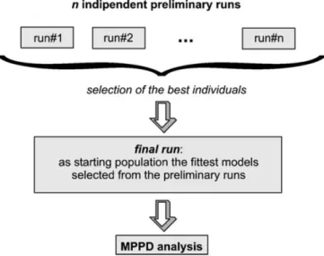
However, in the processing software used, the method used for the inversion of the dispersive curve is based on an optimization process (genetic algorithms) [Dal Moro, 2007).] This method implemented a two-step inversion, the first one starts with several preliminary “parallel” runs and the second one uses the previously determined fittest model as starting population. (Figure 2)

Figure 2- Genetic Algorithms sequence for surface wave analysis

The key element for any kind of optimization is the model evaluation, which is performed by means of an objective function that allows a quantitive estimation of the model. For that it’s considered the RMS value of the difference between the observed and calculated phase velocities, i.e. the dispersion curve.

𝑂𝑏𝑗𝑒𝑐𝑡𝑖𝑣𝑒 𝐹𝑢𝑛𝑐𝑡𝑖𝑜𝑛 = −√∑ (𝑣𝑜𝑏𝑠,𝑖− 𝑣𝑐𝑎𝑙,𝑖) 2 𝑛

𝑖=1 𝑛

(16)

5

where 𝑛 represents the number of observed frequency– velocity couples, 𝑣𝑜𝑏𝑠,𝑖 the observed phase velocity at the 𝑖th frequency and 𝑣𝑐𝑎𝑙,𝑖 the calculated velocity for the considered model (individual of the current population).

 2D S-wave velocity sections.

If surface wave data are collected in a CMP roll-along acquisition fashion, a 2D S wave velocity section can be generated with gridding software by placing each S-wave profile (𝑉𝑆 versus depth) in the middle of the geophone spread with which it was calculated. [Xia et al., 2004]

1.6. S- waves

𝑉𝑆,30 can be estimated using existing 𝑉𝑆 measurements. The results in terms of 𝑉𝑆,𝑍 i.e. time-average shear wave velocity in the topmost z meters are calculated according to:

𝑉𝑆,𝑍= 𝑍 ∑ 𝐻𝑖 𝑉𝑆,𝑖 𝑁 𝑖=1

in which 𝑁 is the number of layers used for the discretization of the model from the surface to 𝑧 and 𝐻𝑖 and 𝑉𝑆,𝑖 are the thickness and shear wave velocity for each layer 𝑖, respectively. Moreover 𝑉𝑆,𝑍 can be used to compare the expected site amplification for two different shear wave velocity profiles. The Next Generation Attenuation ground motion prediction equations use the shear wave velocity of the top 30 m of the subsurface profile (𝑉𝑆,30) as the primary parameter for characterizing the effects of sediment stiffness on ground motions.

The Caltrans Seismic Design Criteria classifies sites based on VS of the top 30 m of the soil profile (𝑉𝑆30). Sites are divided into the six categories (Soil Profile Types A through F) presented in Table 1.

[Wair, B. R. & DeJong J. T., 2012]

Table 1- Soil Profile Types

Site Class Soil Profile Name 𝑽𝑺𝟑𝟎

A Hard Rock >1500 m/s

B Rock 760 to 1500 m/s

C Very dense rock and Soft Rock 360 to 760 m/s

D Stiff Soil 180 to 360 m/s

E Soft soil <180 m/s

F Soils Requiring Site Specific Evaluation -

(17)

6

1.7. Purpose and objectives of the survey

This survey was performed in a construction landfill, aiming to evaluate the dynamic response of the soil, through the estimation of the shear wave velocities. The velocities of the shear waves were obtained from the Rayleigh wave’s dispersion using the Multichannel Analysis of Surface Waves method (MASW). Additionally, and because the method uses vertical impulse and vertical recording, it was also possible to determine the compressional wave velocity (from refraction analysis).

(18)

7 2. SITE CONDITIONS

As said before, the location and identification of the survey area in this study is confidential, so the geological context, as well as its representation, will be without coordinates or other identifying information.

2.1. Topography and Geomorphology

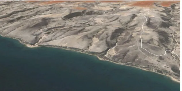
The survey area is near the coastline represented in Figure 3. Onshore site develops according to the continental tectonics, where erosion landforms are structural plains, which were built due to the slow increase of the sedimentary thickness of the crust and the continuous rise of the water level. The site is mainly on the highlands of flat top surface with an absolute elevation of over 200 m, known as a plateau, which belongs to one type of structural plain. The site gradually becomes hilly terrain from east to west and develops into coastal cliffs when meeting the coastline. Some parts of the site are explored areas of limestone which develop karst topography such as cavities, sink holes and slump zones. Concerning the mass movements, a large number of seasonal streams flow from east to west, where the drainage patterns across the site are typically dendritic and are characterized by irregular branching of tributary control.

The coastline is made up of long sandy beaches interrupted by rocky shores and steep cliffs that rise about 120 meters above sea level. The offshore site develops coastal erosion landform, whose type is called wave cut terrace – this inclines towards the sea and its outer edge and is roughly parallel to the coastline.

(19)

8

2.2. Regional Geology

The regional geology is dominated by Proterozoic formation, whilst Neoproterozoic formation occurs in the western part of the country. The onshore section is characterized by a transformed margin which has a distinctive, mainly progradational stratigraphic architecture with long-term sedimentary gaps and high-elevation marine terraces resulting from moderate Upper Cretaceous–Cenozoic to major Quaternary uplifting. Margin style also governs spatial variations in the volume of offshore sediment dispersed in the associated deep-sea fans.

The age and lithology of the geological formations existing in the survey area are the following:

 Holocene marine deposits: sand, gravel, clay, etc.

 Cenomanian-turonian: oolitics and pisolitic limestones, marl (mudstone) and conglomerate.

 Cenomanian: limestone, oolites, dolomite and conglomerate.

 Albian: limestones, marl (mudstone) and gypsum conglomerates.

 Apcian: marl (mudstone), limestone and gypsum.

2.3. Field Tests and landfill construction

A geotechnical survey was conducted in the area before the construction of the landfill, including drilling, in situ tests, SPT, sampling and laboratory tests.

That investigation classified the site stratigraphic according to the following: Soil layers:

a. Marine deposits;

b. Loose, fine-grained, silty sand; c. Very soft clay.

Rock units:

d. Moderately weathered Limestone; e. Moderately weathered Mudstone;

Before the construction of the landfill, the harbor basin was dredged. After the excavation, there were mainly two sorts of rock units: moderately weathered limestone (d) and moderately weathered mudstone (e).

(20)

9

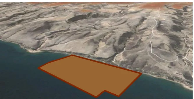
Figure 4- Location of the area after the construction of the landfill. (Image adapted from Google Earth)

2.4. Compaction of the landfill

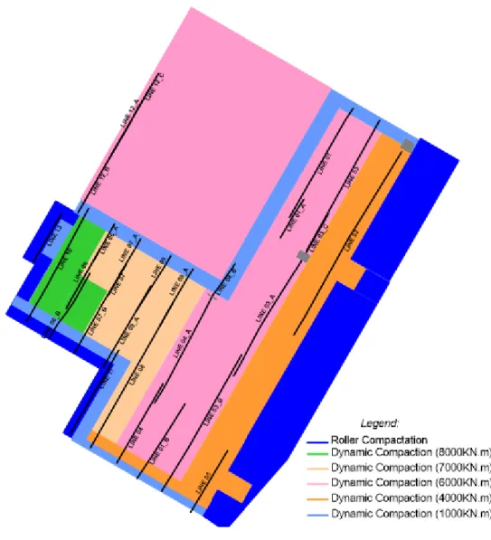
During the construction, the landfill was compacted. The aim of the compression of the landfill is to increase the resistance to the strain disturbance of the soil under the action of external forces; reduce possible volumetric variations, reducing the empty spaces and consequently the water absorption capacity and the percolation decreases, making the soil more stable.

There is no information regarding the moisture content, but concerning the area compression, Figure 5 shows a representative scheme of the compression energy inherent to the survey area. [Das, B. M., (2010)].

(21)

10

Figure 5- Disposition of the different compaction energies along the survey area.

The primary technique used in the compaction of the landfill was the dynamic compaction. This process consists primarily of dropping a heavy weight repeatedly on the ground at regular intervals. The weight of the hammer used varies over a range of 80 to 360 kN, and the height of the hammer drop varies between 7.5 and 30.5 m. The stress waves generated by the hammer drops aid in the densification. The degree of compaction achieved at a given site depends on the following three factors: 1). Weight of hammer; 2). Height of hammer drop and on the 3). Spacing of locations at which the hammer is dropped. However there are no references regarding this values. [Das, B. M., (2010)].

(22)

11 3. DATA ACQUISITION

The present document reports the acquisition and processing of 28 seismic profiles, acquired between March and July 2015, using geometries favorable to the refraction and MASW methods.

The survey was conducted along the profiles shown in Figure 6 and, despite the acquisition orientation, the seismic lines are mostly oriented NNE-SSW with a maximum length of 354 m.

(23)

12

3.1. Equipment and Data Acquisition Parameters

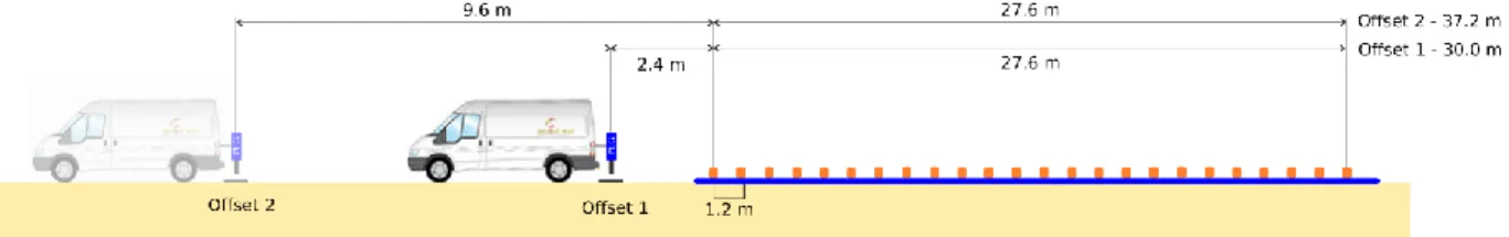
The equipment and data acquisition parameters were carefully selected in order to meet the requirements and goals of the project. The energy was generated by two different sources used during the survey: the Accelerated Weight Drop (AWD) seismic source PEG-40 and the sledgehammer + base plate. The source used for each shot was selected according to the weather and site conditions/limitations. The land streamer used had 24 channels (vertical geophones) spaced 1.2 m, with a total active length of 27.6 m, and the recorder was an exploration seismograph Geode 24 channels (Figure 7). The acquisition parameters are summarized in Table 2.

Table 2– Equipment and data acquisition parameters.

Source 1 AWD PEG 40

Weight 40 kg

Number of stacked Shots per offset 1-2

Source 2 Sledgehammer

Weight 5 kg

Number of stacked Shots per offset 5

Shot Offset 2.4, 9.6 m

Streamer Land Streamer

Number of channels 24

Geophone Interval (GI) 1.2 m

Total Active Length 27.6 m

Geophone OYO 10 Hz

Geophone Type Vertical

Recorder Geode 24 from Geometrics

Sampling Rate 0.125ms

Record Length 1.5 s

Format SEG-2

GPS Trimble R8 DGPS receiver with base station

(a) (b)

(24)

13

3.2. Geometry

To process the refraction data, Rayfract® software was used. This has the particularity of using station numbers, instead of real distances, to define the shots and geophones’ positions. Regarding that fact, the geophones’ spacing of 1.2 m was used as the measuring unit of all the remaining positions/distances. To accomplish this limitation, a multiple offset geometry was used, along with the source and the first geophone distanced by 2.4 m and 9.6 m, respectively offset 1 and offset 2 (Figure 8). The multiple offsets, at 2.4 m and 9.6 m, had the aim of increasing the resolution on shallow layers and of achieving greater depths of investigation, respectively.

For the refraction P wave, two shot offset were processed, however, for the MASW, only the larger shot offset was used to guarantee the desired investigation depth.

In order to increase the signal to noise ratio, for each offset 2 or 5 shots were stacked, according to the selected source (2 stacks using PEG-40 and 5 with the sledgehammer).

Figure 8 – Offset diagram of the seismic spread used for the survey (not to scale).

The space increment along the line was set at 4.8m (spread advance in line); meaning, when the two shots for that spread position are executed, the system is moved forward 4.8m and a new set of shots, in the 2 different offsets, are executed (Figure 9).

The raw recorded data has the geometry assigned for each shot in distance. These distances were converted into stations with intervals of 1.2 m (minimum station spacing). Figure 9 shows the relation between source and receiver positions and their respective distances and station numbers.

(25)

14

Figure 9– Source (blue) and receiver (orange) geometry for 4 shot positions showing the distance between shots, geophones and the stations used for processing.

Station number 23 22 21 20 19 18 17 16 15 14 13 12 11 10 9 8 7 6 5 4 3 2 1 0 -1 -2 -3 -4 -5 -6 -7 -8 -9 -10 -11 -12 -13 -14 -15 -16 -17 -18 -19 -20 Distance (m) -27.6 -26.4 -25.2 -24.0 -22.8 -21.6 -20.4 -19.2 -18.0 -16.8 -15.6 -14.4 -13.2 -12.0 -10.8 -9.6 -8.4 -7.2 -6.0 -4.8 -3.6 -2.4 -1.2 0.0 1.2 2.4 3.6 4.8 6.0 7.2 8.4 9.6 10.8 12.0 13.2 14.4 15.6 16.8 18.0 19.2 20.4 21.6 22.8 24.0 Shotposition 1 G24 G23 G22 G21 G20 G19 G18 G17 G16 G15 G14 G13 G12 G11 G10 G9 G8 G7 G6 G5 G4 G3 G2 G1 S1 S2 Shotposition 2 G24 G23 G22 G21 G20 G19 G18 G17 G16 G15 G14 G13 G12 G11 G10 G9 G8 G7 G6 G5 G4 G3 G2 G1 S3 S4 Shotposition 3 G24 G23 G22 G21 G20 G19 G18 G17 G16 G15 G14 G13 G12 G11 G10 G9 G8 G7 G6 G5 G4 G3 G2 G1 S5 S6 Shotposition 4 G24 G23 G22 G21 G20 G19 G18 G17 G16 G15 G14 G13 G12 G11 G10 G9 G8 G7 G6 G5 G4 G3 G2 G1 S7 S8

Acquisition reference point (middle of the streamer) Shot offset

Geophone position Sequence progression

(26)

15

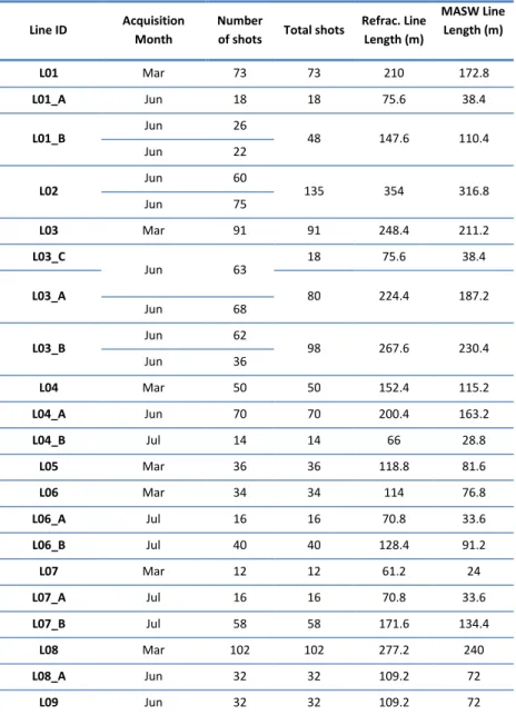
3.3. Line Identification

The lines were identified by the line number (e.g. L01) followed, if applicable, by the portion of the line “_A” or “_B” stem (e.g. L01_A). The following table (Table 3) shows the line ID used henceforth in this report, the month of acquisition, the number of shots, the line length in meters for both methodology refraction and MASW. Some of the lines acquired in different days were merged whenever they match the following criteria:

 Correspondence to a continuation of a previous line (have the same alignment, without a lateral shift);

 Have the same topography (the topography did not change due to an addition of construction landfill material);

 The lines are acquired within a short period of time in order to have a similar level of compaction and water content.

Table 3 - Line identification from acquisition and processing ID. Line ID Acquisition

Month

Number

of shots Total shots

Refrac. Line Length (m) MASW Line Length (m) L01 Mar 73 73 210 172.8 L01_A Jun 18 18 75.6 38.4 L01_B Jun 26 48 147.6 110.4 Jun 22 L02 Jun 60 135 354 316.8 Jun 75 L03 Mar 91 91 248.4 211.2 L03_C Jun 63 18 75.6 38.4 L03_A 80 224.4 187.2 Jun 68 L03_B Jun 62 98 267.6 230.4 Jun 36 L04 Mar 50 50 152.4 115.2 L04_A Jun 70 70 200.4 163.2 L04_B Jul 14 14 66 28.8 L05 Mar 36 36 118.8 81.6 L06 Mar 34 34 114 76.8 L06_A Jul 16 16 70.8 33.6 L06_B Jul 40 40 128.4 91.2 L07 Mar 12 12 61.2 24 L07_A Jul 16 16 70.8 33.6 L07_B Jul 58 58 171.6 134.4 L08 Mar 102 102 277.2 240 L08_A Jun 32 32 109.2 72 L09 Jun 32 32 109.2 72

(27)

16

3.4. Navigation and Positioning

A criterious positioning procedure was made. The topographic survey was carried out using a RTK system. A measurement (x y, and z) was performed at the 1st shot position and for geophones 1, 12 and 24 (G01; G12; G24; S01 in Figure 9); at the last shot position and again for geophones 1, 12 and 24 (G01’; G12’; G24’; S##’); and in areas with curves in the profile and topographic variations, such as trenches or slopes (Figure 10). The positioning was based on the WGS84 datum and the elevations are relative to Mean Sea Level (MSL).

Figure 10- Representation of the measurement positions acquired according to the topographic

variations. The blue points represent shot positions and the red ones geophone positions in the landstreamer.

Although the survey area is relatively flat and all the lines range from 2 to 4 m above sea level, the same profile of the topographic variations is always less than 1 m.

3.5. Data Acquisition Constraints

During daytime there was construction work in progress on the site. Therefore, the MASW survey was conducted at night in order to avoid ambient/seismic noise. The acquisition was sometimes constrained by obstacles in the planned lines, adverse weather conditions and infrastructures, such as trenches (Figure 11). Small curves or even small spatial shifts from the planned profile were made when it was necessary to bypass some obstacles (vehicles or pavement bricks - Figure 12).

L09_A Jul 52 52 157.2 120 L10 Jun 70 70 214.8 177.6 L11 Jul 54 54 162 124.8 L12_A Jul 42 42 133.2 96 L12_B Jul 60 60 176.4 139.2 L12_C Jul 18 18 75.6 38.4 L13 Jul 26 26 94.8 57.6

(28)

17

For example, in the case of a trench, besides the position of the geophones G01, G12 and G24, other geophone positions had to be measured in order to get all the topographic variations.

(a) (b)

Figure 11 – Example of topographic constraints: (a) trench and (b) topographic slope.

(a) (b)

(29)

18 4. SIGNAL ANALYSIS

In order to ensure that the data could be processed successfully, all the acquired seismic data underwent a thorough quality control procedure of the signal quality, positioning and acquisition geometry. The following QC was implemented for each line:

 Refracted wave check for selected shots by a shot to gather analysis;

 Noise analysis and signal saturation assessment;

 Positioning quality control – the lines have to follow some requirements, such as overlapping with previous acquired profiles, matching what was planned or, if the profiles do not match due to constraints/obstacles in the field, they should have been approved;

 The geometry needs to be respected and checked before processing. Therefore, the source and receiver offset was controlled for each land shot, in order to ensure that the chosen geometry was preserved.

4.1. Source Analysis

Due to the weather conditions, the landfill was muddy, which made it difficult to use of the van and, consequently, the PEG-40. As a result, some shots had to be done with another source – the sledgehammer. In the L03, eight shots (10169-10176) were acquired with a sledgehammer. Hence, in order to understand which frequency is generated from the two sources, the frequency spectrum of the sources is described below (Figure 13).

(30)

19 (b)

Figure 13 – a) Frequency spectrum of Source 2-Sledgehammer regarding the 10070 of L03 and b) Frequency spectrum of Source 1-PEG 40 regarding shot 10018 of L03.

The amplitude spectrum analysis allows the identification of the dominant frequency or period corresponding to the maximum amplitude value. Considering the two spectrums, it is possible to conclude that PEG-40 has a higher dominant frequency than that of the sledgehammer. In both cases, the frequency was limited to the highest amplitudes for the processing.

4.2. QC Data Issues

During the QC analysis, some issues were detected in the data:

 Some data was affected by low frequency resonance depredating velocity spectrum and, therefore, making the dispersion curve picking impossible. This issue is identified in:

o Shots 10010 and 10022 of L3 (Figure 14 – a) and b) respectively); o Shot 10052 of L8 (Figure 14 – c).

 Some shots were also affected by the plate’s vibration, due to the coupling of the base plate to a hard surface, leading to a rebound of the base plate and causing subsidiary pulses and ringing effects:

o Shot 10010 of L11 presents high frequency noise; therefore, this profile was processed in MASW using the maximum frequency content of 50 Hz (Figure 14 – d));

o Shot 10026 of L13 was not processed in MASW because it shows multiple pulses caused by the plate’s vibration (Figure 14 – e)).

(31)

20 (a)

(b)

(32)

21 (d)

(e)

Figure 14 – Phase velocity spectrum on the left and frequency spectrum on the right for a) L3 shot 10010; b) L3 shot 10022; c) L8 and shot 10052; d) L11 and shot 10010 and e) L13 and shot 10026.

(33)

22 5. SEISMIC DATA PROCESSING

Twenty-eight seismic profiles were processed using MASW and refraction methodologies were used, respectively, winMASW® and Rayfract® software. The generic processing flow applied to the data was organized as in Figure 15. All the shots were used in the refraction methodologies, whereas, in the MASW, only the far offset shots were processed.

Figure 15 - Processing workflow applied to the seismic lines. Rounded boxes represent the processing steps and grey boxes represent the input/output products.

The use of the refraction processing was crucial for the MASW processing, because without an a priori processing to establish near surface structure (velocity and thickness), the dispersion of the results after inversion was tremendous.

(34)

23

5.1. Refraction Processing

The seismic refraction processing was done using Rayfract® software after importing the following data (Figure 15):

- SEG-2 with nominal geometry assigned; - Topographic insertion.

The processing in Rayfract® included the picking of the first arrival (Figure 16), for every shot and every channel where the SNR allows accurate picking.

The analyses of the first arrival picking was done for every line, allowing a minimal RMS error of the Rayfract models (see Appendix A: Notation used)

Figure 16– Shot gathered analysis (shot 10010, l01) for refracted wave analysis.

A 2D compressional wave velocity model in grid format (*.grd) was obtained for each line plotted using

the Golden Software's Surfer® (see Figure 17, using the Delta-t-V method. This pseudo-2D turning ray

inversion method was chosen because it delivers continuous 1D depth 𝑽_𝑺. velocity profiles for all profile stations and it has a better vertical resolution than the other inversion methods available in the software.

The 2D compressional wave models were used to infer the thickness/geometry of the layers, as preliminary input for MASW data processing/modeling (see Figure 18).

(35)

24

Figure 17 - 2D compressional wave velocity model obtained fom L01.MASW Processing

For each shotpoint with 9.6 m S/R offset, a 1D 𝑽𝑺 vertical velocity model was located in the middle of

the spread between the 12th and the 13th geophone (see red star in Figure 9). The source offset of 2.4m wasn´t used because it would not cover the desired investigation depth.

5.1.1. Model Creation

Since the objective is to characterize the landfill, the upper velocity limit of the 2D compressional wave velocity model was defined at 𝑽𝑷=𝟑𝟓𝟎𝟎 𝒎𝒔−𝟏 for each line. The lower limit wasn´t standard because the 𝑽𝑷𝒎𝒊𝒏 was different for each model. However, the thicknesses of each layer 𝒉 range were around 500 𝒎𝒔−𝟏 (see Figure 18 ) in order to establish the surface layers of the 1D 𝑽_𝑺 vertical velocity model.

Figure 18 - Initial thickness model created for shot 10006 of L01. Note that the representative point for each shot is located 23.4 m from the shot’s position, as exemplified in Figure 9.

(36)

25

Table 4- Thickness model used for shot 10006

𝑽𝑷 (𝒎𝒔−𝟏) 𝒉 (𝒎) - 500 2.3 500 - 1000 2.8 1000 - 1500 2.2 1500 - 2000 1.5 2500 - 3000 1.4 3000 - 3500 1.6 3500 - ∞

5.1.2. Velocity Spectrum and dispersion curve picking

For each shot, superficial waves were selected (Figure 19) to represent the velocity spectrum.

Figure 19 - Shot gathered analysis (shot 10010, l01) for refracted wave analysis - selection of the surface waves.

The velocity spectrum corresponds to an energy scatter plot that relates the frequency with the phase velocity for surface waves.

(37)

26

For picking the dispersion curve, the points that belonged to a particular propagation mode of a surface wave were selected and the fundamental mode (Figure 20) was picked in the f-v domain. Sometimes, the interference of different modes can alter the apparent dispersion characteristics of the fundamental mode or result in higher modes being misinterpreted as fundamental. Therefore, the picking was only made up until the interference of a higher mode.

All the 1D shear wave models resulted from the fundamental vibration mode picking of the velocity spectrum. Besides that, sometimes, a higher mode can be visible in the data such as in Figure 20, yet it wasn't consistent in all data.

Figure 20 –Picking of the fundamental vibration mode – dispersion curve in the F-V domain.

After the picking in the f-v domain, it is possible to see the dispersion curve in the f-k spectrum (Figure 21).

(a) (b)

(38)

27

5.1.3. Maximum depth penetration

The maximum penetration depth in a homogeneous medium is about one wavelength. The currently accepted rule of thumb for the maximum penetration depth is approximately half of the longest wave length (λ/2) or (λ/2.5) [Elisoft – geophysical software and services, 2015]. This value is the outcome of the relationship between velocity and the frequencies represented in the dispersion curve:

λ=𝑉𝑓 𝑓

Table 5 - Relation between wave length and maximum depth penetration, relatively to the dispersion curve of shot 10006 of

L01 (see Figure 20) F (Hz) Vf (m/s) λ (m) Depth (m) 19.484 395.000 20.273 8.109 10.136 20.649 352.370 17.065 6.826 8.532 22.719 317.599 13.980 5.592 6.990 26.729 295.272 11.047 4.419 5.523 31.387 289.546 9.225 3.690 4.613 35.915 290.107 8.078 3.231 4.039 40.185 292.611 7.282 2.913 3.641 44.584 295.915 6.637 2.655 3.319 48.853 299.264 6.126 2.450 3.063 52.476 301.971 5.754 2.302 2.877 55.839 304.226 5.448 2.179 2.724 59.203 306.081 5.170 2.068 2.585

In this particular shot, the maximum penetration depth was approximately 10 m.

5.1.4. Modeling and Inversion of the dispersion curve

The initial thickness model created, based on the refractive method, is introduced at this stage of processing (Figure 18), and then adjusted to the velocities of each layer and bedrock to adjust to the velocity spectrum (Figure 22).

(39)

28

Figure 22 – Introduction of the initial thicknesses model based on the refraction method.

Table 6- Initial 𝑽𝒔 profile used for shot 10006

𝑽𝒔 (𝒎𝒔−𝟏) 𝒉 (𝒎) 340 2.3 280 2.8 320 2.2 400 1.5 520 1.4 650 1.6 700

_∞

Having finalized the adjustments of the model to the dispersion curve, the second phase was the inversion of the model created. This inversion is made by means of an optimization process (genetic algorithms) that requires the computer a big calculation effort. (Dal Moro et all, 2007)

In the inversion, two 1D 𝑉𝑆 models were obtained: the “best” model (in terms of lower misfit, i.e the discrepancy between the observed and the calculated curve) and a medium model calculated by means of MPPD (Marginal Posterior Probability Density). However, just the best model was considered further on. The next figure shows the results of the first inversion. (Figure 23)

(40)

29

Figure 23 –First inversion results: Velocity spectrum and dispersion curve (a); misfit evolution (b); and 1D shear wave velocity model obtained for L1 for shot 10006.

To improve the results, namely the misfit evolution of the model to the velocity spectrum, a second inversion was made with the best output of the first inversion – the best model. In this inversion, its limits were adjusted to achieve a better approximation with the dispersion curve.

The next figure shows the results of the second inversion. (Figure 24)

Figure 24 –Second inversion results: Velocity spectrum and dispersion curve (a); misfit evolution (b); and 1D shear wave velocity model obtained for L1 for shot 10006.

(41)

30

As it was expected, the error decreases, reaching a “misfit evolution" of 1% between the “fittest model” and the dispersion curve.

5.1.5. Model Validation

The 1D shear wave velocity model obtained in the second inversion must be compared with the dispersion curve of the fundamental mode in order to determine if the misfit is satisfactory (Figure 25).

Figure 25– Comparison between the dispersion curve and the final model created

For the interpolation, each and every S-wave profile (𝑉𝑆 versus depth) was displaced/ incremented with its respective topographic elevation, as represented in Figure 26. Also, the layer thickness, given by the software winMASW®, was converted to the depth of half of the layer, considering 2 points for the first layer (1/2 layer and the topography), both with the same velocity and a middle point for the remaining layers (see example in Figure 26).

(42)

31

Figure 26– Example of a conversion from layer thickness given by the 1D model to the depth of half a layer used to generate the 2D shear wave velocity models.

To generate a 2D 𝑉𝑆 section, all 1D 𝑉𝑆 models per line are interpolated and plotted using Golden Software's Surfer®

(43)

32 6. RESULTS AND DISCUSSION

The 2D shear wave velocity section was obtained for each profile using Golden Software's Surfer® and interpolating all 1D 𝑉𝑆 models of the respective line (Figure 26). The interpolation was performed using the Triangulation methodology (Golden Software, Inc, 2014) with a spacing of 0.2 m and anisotropy ratio of 5. The model was filtered using a low pass filter (moving average) with a filter size of 3 rows x 5 columns.

The lines were plotted from southwest (SW) to northeast (NE), independently of the acquisition orientation.

For a better perception of the evolution of the dynamic properties of the soil along the landfill, all the 28 2D shear velocity models were paced in its locations and represented by a 3D software - Voxler 3® by Golden Software, on a representative scheme of the area under study.

In addition to that, every model has its own 𝑉𝑆30 graphic on top, rightly placed. This value it’s an output of the software winMASW for every 1D 𝑉𝑆 profile. This estimation, however, goes beyond the maximum penetration depth, so after the layer stratification, the bedrock is assumed with the same shear wave velocity until the 30 m of depth.

(44)

33

(45)

34

Concerning the sea location, at northwest from the survey, it is possible to see the deepening of the bedrock towards the sea. However, the landfill is at the same height relative to the average level of the sea water due to the higher thickness of sediments above.

Regarding the acquisition time, the lines acquired in March (rainy season) (Table 3) present lower velocities above the bedrock, this is probably due to the high water content in the landfill in that time season. On the contrary, as expected, the remaing lines, in general, present higher velocities in the landfill. However, closest to the sea, the shear waves velocities models tend to decrease its velocities in the landfill, for example L04_B, L12_B, L12_A, etc. (Figure 6 and Figure 27).

Besides, several elements may affect the shear wave’s velocities, such as tides, uneven compression in the landfill, different soils, which can lead to different elastic properties, etc.

A deeper analysis could be done to each shear wave velocity model, so three profiles were chosen to compare L01, L02 and L06 (Figure 28 and Figure 29-b)).

Figure 28–shear wave velocity model for a) L01 and b) L06 resultant from the interpolation of all 1D 𝑽𝑺 models obtained

(46)

35

The purpose of comparing L01 and L06 is to understand the influence of different compaction energies (Figure 5) on shear wave velocities. For that effect, the lines were acquired in the same season to eliminate other factor influences.

Analyzing these two models, the differences in the depth of the bedrock is clearly visible, changing approximately 5 m. The minimum shear wave velocity achieved in both models is not significant. In model 06, 𝑉𝑆𝑚𝑖𝑛= 217 𝑚/𝑠 where as in model 01, 𝑉𝑆𝑚𝑖𝑛 = 245 𝑚/𝑠.

However, despite the L06 being acquired in a zone with higher compaction energy (7000-8000 kNm) than the L01 (6000 kNm), the shear wave velocities in L06 are lower than in L01. Perhaps the proximity of the sea may have a greater influence than the compaction energy made on site or the materials used in each section of the landfill were different, having consequently a different responses.

The purpose of comparing L01 and L02 is to understand the influence of the rainy season in the landfill behavior. Comparing this two models, the minimum velocity in L01, as it was already said above, is 𝑉𝑆𝑚𝑖𝑛= 245 𝑚/𝑠, where as in model 02, 𝑉𝑆𝑚𝑖𝑛= 293 𝑚/𝑠. The lines acquired in June reveals higher minimum velocities (almost 50𝑚/𝑠) than the one acquired in March, even though L01 being located in a bigger energy compaction zone.

6.1. 𝑽𝑺𝟑𝟎 Analysis

All the lines analyzed present a 𝑉𝑆30 above 360 𝑚/𝑠, which means that, by Caltrans Seismic Design Criteria, all the soils are considered in the site class C - Very dense soil and soft rock.

However, there are some diferences between the lines. For instance, there are models with very low values for the 𝑉𝑆30, such as L04_B, L10, L11 and L13 and models with a great variety, like L02 or L07_B. Althought, the lack of information regarding the site, namely the soil conditions and composition prevent a deeper analysis.

6.2. Tides Influence

Finally, to exemplify the tides influence in the shear wave velocities models, due to the water level variation, I used L02 to make this analysis because it was acquired in two different days.

Analyzing the log acquisition of this line (Table 7), regarding the day and hour, a tides plot for each day was taken and plotted (Figure 34). These tides plots relate the sea level, in meters, with the time of the day, indicating also the high and low tides periods.

For a better visualization and characterization, the tides plot were edited and selected for the acquisition period of each shot (Figure 29).

(47)

36

Table 7 - Acquisition log for L02

Station File name Date Hour

-8 10002 1st_{acq. day} _2:02 -12 10004 1st_{acq. day} _2:09 -16 10006 1st_{acq. day} _2:16 -20 10008 1st_{acq. day} _2:21 -24 10010 1st_{acq. day} _2:25 -28 10012 1st_{acq. day} _2:30 -32 10014 1st_{acq. day} _2:38 -36 10016 1st_{acq. day} _2:43 -40 10018 1st_{acq. day} _2:48 -44 10020 1st_{acq. day} _2:54 -48 10022 1st_{acq. day} _3:04 -52 10024 1st_{acq. day} _3:08 -56 10026 1st_{acq. day} _3:14 -60 10028 1st_{acq. day} _3:20 -64 10030 1st_{acq. day} _3:24 -68 10032 1st_{acq. day} _3:29 -72 10034 1st_{acq. day} _3:34 -76 10036 1st_{acq. day} _3:37 -80 10038 1st_{acq. day} _3:43 -84 10040 1st_{acq. day} _4:53 -88 10042 1st_{acq. day} _5:00 -92 10044 1st_{acq. day} _5:12 -96 10046 1st_{acq. day} _5:16 -100 10048 1st_{acq. day} _5:22 -104 10050 1st_{acq. day} _5:26 -108 10052 1st_{acq. day} _5:32 -112 10054 1st_{acq. day} _5:36 -116 10056 1st_{acq. day} _5:45 -120 10058 1st_{acq. day} _5:55 -124 10060 1st_{acq. day} _6:01

Station File name Date Hour

-128 10062 2nd_{acq. day} _2:30 -132 10064 2nd_{acq. day} _2:35 -136 10066 2nd_{acq. day} _2:39 -140 10068 2nd_{acq. day} _2:43 -144 10070 2nd_{acq. day} _2:47 -148 10072 2nd_{acq. day} _2:51 -152 10074 2nd_{acq. day} _2:54 -156 10076 2nd_{acq. day} _2:59 -160 10078 2nd_{acq. day} _3:09 -164 10080 2nd_{acq. day} _3:12 -168 10082 2nd_{acq. day} _3:16 -172 10084 2nd_{acq. day} _3:30 -176 10086 2nd_{acq. day} _3:34 -180 10088 2nd_{acq. day} _3:37 -184 10090 2nd_{acq. day} _3:42 -188 10092 2nd_{acq. day} _3:48 -192 10094 2nd_{acq. day} _3:51 -196 10096 2nd_{acq. day} _3:54 -200 10098 2nd_{acq. day} _3:58 -204 10100 2nd_{acq. day} _4:01 -208 10102 2nd_{acq. day} _4:04 -212 10104 2nd_{acq. day} _4:10 -216 10106 2nd_{acq. day} _4:23 -220 10108 2nd_{acq. day} _4:26 -224 10110 2nd_{acq. day} _4:30 -228 10112 2nd_{acq. day} _4:34 -232 10114 2nd_{acq. day} _4:38 -236 10116 2nd_{acq. day} _4:41 -240 10118 2nd_{acq. day} _4:48 -244 10120 2nd_{acq. day} _5:08 -248 10122 2nd_{acq. day} _5:14 -252 10124 2nd_{acq. day} _5:17 -256 10126 2nd_{acq. day} _5:25 -260 10128 2nd_{acq. day} _5:28 -264 10130 2nd_{acq. day} _5:31 -268 10132 2nd_{acq. day} _5:35 -272 10134 2nd_{acq. day} _5:38

(48)

37

Figure 29 - Tides plot (above) regarding the acquisition time of the shots. Note that the line's acquisition begins on the right side (1st_{Acquisition day); after the shot 10060, the line was}

(49)

38

As we can see the tides level has a real impact in the shear wave velocity model, a lower velocity layer follows the tides level along the line, reaching a maximum elevation in the highest tides, in both days. Furthermore, the differences in tides level is visible in the shear wave’s velocity (transition between shots 10060 and 10062). However, the differences in the tides only change the saturation level, because a higher zone still affected with water.

6.3. Elastic Modulus

[Mavko, G. et al, 2009]

summarizes some popular and useful 𝑉

𝑃

− 𝜌. Density is a simple

volumetric average of the rock constituent densities and is closely related to porosity by:

𝜌

_𝑏

= (1 − 𝜙)𝜌

₀

+ 𝜌

_𝑓1

where 𝜌

0

is the density of mineral grains, 𝜌

𝑓1

is the density of pore fluids, and 𝜙 is the porosity.

Figure 30 - Both forms of Gardner's relations applied to log and laboratory sandstone data- [Castagna et al., 1993]

Using the equation selected in red, it was possible to estimate the density from the P-wave models. However, this was only an estimation, because the equation is intended for consolidated rocks, wich is not the case of landfill in study. Above it is the result of the density model calculation using the equation referred.

The following profiles (Figure 31 & Figure 32) were disposed with a vertical scale of 1:15 and a horizontal scale of 1:30.

(50)

39

Figure 31 – 2D Density model calculated to L01 from the 2D P-wave velocity model of the same profile.

With the density values calculate, it is already possible to achieve the shear modulus (Figure 32), through the formula: 𝐺𝑚𝑎𝑥= 𝜌𝑉𝑆2. However, due to the high uncertainties and approximate equations, this is only an example, not being calculated for all profiles performed in the landfill.