Sonae Indústria : equity valuation

(1)

Sonae Indústria

Equity Valuation

Mafalda Fortunato de Almeida Espiñeira

Nr 152109329

(2)

Abstract

The objective of this dissertation is valuing Sonae Indústria, the second largest wood panel payer in the world, using the most appropriate valuation approaches. Being field of valuation exceptionally complex, it is crucial to address the main issues and mechanisms behind an equity valuation.

In order to do this, I will analyse the main valuation methods and theories of academic literature as well as advantages and disadvantages. Afterwards, I compare with Millennium Investment Banking, explaining the main differences in assumptions as well as methodology used.

(3)

Acknowledgments

I would like to express my sincere gratitude to Professor José Tudela Martins, the Dissertation Advisor who contributed for the final quality of my work as well as for all availability; to Mrs. Catarina Castro, Mr. Diogo Pimentel, Mr. Luis Santos and all team of Santander Asset Management for all contributions, recommendations and knowledge and expertise that they gave me; to my friends of the Equity Valuation workshops, namely Francisco Pereira dos Santos, Catarina Mourinho and Ricardo Ortigão Ramos; all my friends and family.

(4)

1 -

Introduction

The purpose of this dissertation is to determine the equity value of Sonae Indústria, linking theoretical frameworks and practice. Therefore, the dissertation will be presented four parts: the literature review that give us a background about the field of valuation its principal valuation approaches and their advantages and disadvantages; a brief description of company as well as its strategy and future trends; Sonae Industria’s valuation where it is include assumptions in order to reach the equity value; the last one, it will made a comparison with Millennium Investment Banking.

(6)

2 - Literature Review

“Every asset, financial as well as real, has a value” and “ any asset can be valued” (Damodaran, 2002). All valuation methods have the same goal: to find the value of the firm.

2.1 - Overview

Valuation plays an important role in several areas of Finance, from Mergers and Acquisitions (M&A) to portfolio management. As Damodaran (2006) declares “Valuation can be considered the heart of finance”.

Before developing the valuation of any company, it is crucial to address the main issues and mechanisms behind an equity valuation. As Copeland et. al (2000) argues that valuation permits business managers to make value-increasing decisions, enhance strategic and financial decision making and, consequently, create value to maximize shareholder value.

Fernández (2007) also stated that valuation is a key factor of corporate finance, recognizing the importance of valuation as a mean to identify its business units that help to generate and to destroy economic value within the company.

Behind every major resource-allocation decision in a company lays some calculation of what it is worth. The resource-allocation process presents three types of valuation problems, as managers need to be able to value operations, opportunities and ownership claims. Although valuation is always a function of three factors: cash, timing and risk. (Luerhman, 1997)

The field valuation is extremely vast, complex and subjective. As Young el al. (1999) declares, there is “valuation overload”, which means that there is a large variety of different approaches, each one with its own assumptions, advantages and disadvantages.

(7)

Indeed, there is not a unique path to get to the final value of a set of assets or a company. Depending on the nature of the company, the information available and the purpose of the valuation, we should choose the methods that can be considered preferable, most accurate in determining the value (Booth, 2007). So, the first step in valuation is deciding which valuation method is most appropriate for a given company. Although the end-results are estimated based on quantitative methods, each of these methods/approach requires a different set of assumptions, made by each single analyst which has a subjective perspective. This will be reflected in the final value, i.e., different results for the same company (Damodaran, 2002).

However, all valuation models are no more than a different way of expressing the same underlying asset, which means that they are mathematically equivalent: if we make the right judgments it will lead to similar values. The similarities among models imply four main practical implications: consistency (on the assumptions), comparison (valuation models can be compared directly), uniqueness (one single fair value estimate no matter how many approaches we use) and consistency without uniformity.

If we merge both Damodaran (2006) and Fernández (2007), we can differentiate four types of valuation methods. Firstly, Discounted Cash Flow (DCF) valuation, which relates the value of an asset, it is equal to the sum of the Present Value (PV) of expected future cash flows of that asset; the second one, Liquidation and Accounting Valuation, which is founded on the principle that a firm’s value lies in its balance sheet. This means that the value of assets are not taking into account the future cash flow generate by firm; the third approach, Relative Valuation, estimates the value of an asset by looking at the price of “comparable” assets relative to a common variable like earnings, cash flows, book value or sales; finally, Contingent Claim Valuation that uses option pricing models like Binomial Model or Black and Scholes to compute the value of assets.

(8)

secondly, the value of a risky asset is equals to a certainty equivalent cash flow discounted at a risk free rate. In the third one, we apply an adjusted present value, where the value of a firm is the sum of the value of the business, 100% financed by equity and marginal effects of debt financing. The last is excess returns.

In this section, I will concentrate more on DFC and Relative methods since I will use it in Sonae Indústria valuation, while Contingent Claims and Liquidation approach will not be discussed in detail.

2.2 - Valuation Methods

2.2.1- Discounted Cash Flow (DFC)

Damoradan (2006) states “we buy most assets because we expected them to generate cash for us in the future”. In a DCF approach, we begin with a simple preposition that the value of an asset is not what someone perceives it to be worth but it is a function of the expected cash flows on that asset.

These methods centres on the idea that the value of an asset is the present value of the expected cash flows on the asset, discounted back at a rate that reflects the riskiness of these cash flows.

There are two different approaches in DCF valuation: either value the entire business (firm perspective) or just value the equity stake in the business (equity valuation). We can compute the value of the equity stake through the value of entire business after subtract net debt and minorities interests.

According to Damodaran (2206), this approach is the most used in academia and comes with the best theoretical credentials.

(9)

2.2.1.1 – Firm Valuation Approach

In this variant of the DCF model, we value the firm (entire business) to discount Free Cash Flows to the Firm at a risk - adjusted discount rate.

FCFF is the amount of cash earned by a firm after paying all operation expenses, taxes and reinvestment needs, but before paying any interest or dividends debtholders or equityholders (Damodaran, 2005).

2.2.1.1.1 - WACC

WACC-based model calculates the value of the firm by discounting the expected future cash flows at a rate that represents all financing sources (equity holders, debt holders or both) used to generate these same cash flows, called weighted average cost of capital (WACC).

The formula to calculate a firm’s value is divided in two parts. First, it calculates the present value of expected future cash flows up to a certain point in the future and, second, the terminal value (TV). According to Young, M. et al. (1999, TV is the principal component of firm’s value and very sensitive to changes in the discounted rate or in terminal growth rate.

The WACC can be defined as a tax adjusted discounted rate, which means that it is

(10)

We can find different expressions of the WACC, but the most common are:

Although WACC is one of the most common used valuation methods due to its simplicity, the WACC concept presents some limitations. WACC requires a set of restrictive assumptions that sometimes are not taken into consideration. WACC always works well under assumption that target of debt ratio over firm market value is held constant over that period of time.

As Luerhman (1997) says, “WACC has never been that good at handling financial side effects” and “not very convincingly”. This means that WACC should be adjusted not only to tax shields but also to issue costs, financial distress costs and changes in financial structure. The last adjustment is the one that is usually miscalculated, forgetting the two components to compute the WACC: the cost of equity and the cost of capital, that also changes, since it’s a function of the given capital structure.

An alternative for valuating a firm is to apply the APV method, which is more transparent and adaptable for firms with dynamic and complex capital structure, or to compute the value of WACC every year, but requires a set of assumptions (Koller et al., 2005).

Despite the large amount of critics, WACC is suitable only for the simplest and most static capital structure (Luehrman, 1997).

2.2.1.1.2 – APV

Luerhman (1997) argues that “the better alternative for valuing a business operation is to apply the basis DCF relationship to each of a business’s various kinds of cash flows

(11)

and then add up the present values”, which is called adjusted present value and replaces the WACC as the DCF methodology of choice among generalists.

This method avoids some of the miscalculations that can occur when computing the WACC- based model and can provide relevant information since it “can help managers analyse not only how much an asset is worth but also where the value is comes from” (Luerhman, 1997).

In this approach, we start to compute the value of firm as if it was completely financed by equity. As we add debt to the company, we need to take into account two effects: the benefits of having debt because interest expenses are tax deductible and the costs of borrowing that increase expected bankruptcy costs. The value of firm if it is 100% equity financing is given by:

After calculating the value of the unlevered firm, the next step is to evaluate the expected tax benefit from a given level of debt.

How to discount the effect of tax savings? Based on the initial study of Miller and Modigliani (1963), and recently developed by Cooper and Nyborg 2006), academics conclude that the value of the tax shield is the present value of the interest tax savings discounted back at the cost of debt. According Luerhman (1997), the tax shield should be discounted at a rate that reflects the riskiness of this cash flow, which is the cost of debt.According to Damodaran (2006), the present value of taxes shields formula is the following:

(12)

The last step is estimating expected bankruptcy costs. The expected bankruptcy costs are the present value of the loss in a firm in case of distress and it is not common to appear in the APV formula because the expected bankruptcy costs are difficult to compute (Damodaran, 2006).

As Koller et al. (2005) argues the Enterprise Value is the sum of the different components of value, therefore, the value of a firm can be written as:

For Luerhman (1997) the “APV always works when WACC does, and sometimes when WACC doesn’t, because it requires fewer restrictive assumptions”.

When comparing these two approaches, we can conclude that APV method is more flexible, transparent, providing more information than WACC. However, the main criterion to choose between them is usually the capital structure of firm, i.e. companies with changing capital structures should implement APV approach while firms with static debt ratio will be use WACC.

(13)

2.2.1.1.3 - Capital Cash flow (CCF) valuation

This method is equivalent to the free cash flow of the firm valuation, being the main difference the way that tax shields are treated. In WACC method interest tax shield are excluded from the free cash flows while CCF uses all free cash flows available for capital provides and interest tax shield. This way, CFF discounts these cash flows at a before-tax cost of capital (WACCBT).

As Ruback (2002) affirms, CFF and WACC methods are two different ways of valuing cash flows using the consistent assumptions.

2.2.1.1.4 – Excess return model

Damoradan (2010) argues that, in this type of valuation, the cash flows are split into excess return cash flows and normal return cash flows. The normal return is defined as the earnings the risk-adjusted return (cost of capital or equity) while the excess return is any cash flows above or below this normal return.

The most used model is the Economic Added Value (EVA), which is defined as a measure of the surplus value created by an investment or portfolio of investments.

Economic Value Added = (Return on Capital Invested – Cost of Capital) X (Capital Invested) = After – tax Operating Income – (Cost of Capital) X Capital Invested

However, there are some authors that try to explain that the relationship between this valuation and stock returns is not perfect.

(14)

2.2.1.2 – Equity Valuation Approach

In this valuation approach, the equity stake in the business is the expected future cash flows for the equity investors discounted at a rate that is appropriate for the equity risk in the company.

2.2.1.2.1 - Dividend Discount Model (DDM)

Among all DCF models, Dividend Discounted Model is the oldest variant of discounted cash flows. This method assumes only dividends as cash flows to equity and then discounts them at the cost of equity.

Where:

E (EDSt) is equal to expected dividend per share in period t Ke is equal cost of equity

This model has two main inputs: expected dividends and the cost of equity. In order to compute the expected dividend we need to assume expected future growth in earnings and payout ratios. The cost of equity (ke) is estimated using the CAPM that will be discussed later on.

The DDM benefits from its simplicity, intuitiveness and, as Damodaran (2006) argues, requires fewer assumptions than other DCF approach. Indeed, it presents limitations (Vernimmen, 2005) suchas the difficulty to estimate the growth rate of dividend. Analysts use this method when companies pay a high level of dividends, i.e. in firms with mature business and stable earnings.

(15)

2.2.1.2.2 - Free Cash Flow to Equity (FCFE)

The free cash flow to equity model is one variant of the Dividend Discounted Model; it discounts potential dividends instead of actual dividends. According to Damodaran (1994), free cash flow is the one that “captures the cash flow left over all reinvestment needs and debt payments”.

Where:

FCFEi is the Cash flow generated by the company in explicit period

FCFE = Net Income + Depreciations and Amortizations – Capital Expenditures – Changes in Working Capital – (debt repayments – New Debt issued).

RVn is equal to residual value of the company in the year n Ke= cost of equity

g = expected growth rate these cash flow

Comparing FCFF valuation and FCFE, we can notice that FCFF approach reduces the mistakes concerning the financing structure once FCFF uses a pre-debt cash flow whereas FCFE takes into account debt repayments and new debt issuances (Damodaran, 2006). Indeed, both methods are theoretically equivalent if we make consistent assumptions. I am not going to exploit this method because I will not use it in Sonae Industria’s Valuation.

2.2.1.3 - Issues behind DCF

As mentioned before, the cost of capital reflects not only two financing sources but also the capital structure of firm and taxes (TC).

(16)

2.2.3.1 Cost of equity

In order to estimate the cost of equity, the capital Asset Pricing Model (CAPM) is the most common model among academics. The cost of equity is a function of three components: market risk premium (RM-RF), the beta of the company (B) and risk free rate (RF). Markowitz (1959) was the first academic that related expected return and risk in order to achieve an optimal investment portfolio and later developed by Sharpe (1964) and Lintner (1965). However, there are others ways to compute the cost of equity such as Arbitrage Pricing Theory (Ross, 1976) and Multi-factor model (Fama and French, 1996) but in this section I will focus in CAPM method. Below we can find the equation recommended to calculate cost of equity.

Where:

RF = Risk free rate Bu = Beta unlevered Bl = Beta levered

(Rm – Rf) = Market risk premium

Risk free rate (Rf)

As Damodaran (2008) states, the risk free rate is the return one gets in an “investment where we know the expected return with certainty”, which means that default risk is equal to zero. This author argues that there are two features that have to be considered. The first one is that “there can be no default risk”. The second is that there has to be “ no reinvestment risk”. Thus, the only securities that don’t have default risk associated with the reinvestment are the government security, precisely zero-coupon

(17)

bonds. In addition, the risk free asset must have the same, or close, to the time to maturity as the investment.

Finally, the risk free rate should be consistent with the cash flows in terms of currency due to the levels of inflation. For example, countries where the inflation is stable, it is more appropriate nominal rates while in countries where this indicator is more volatile, real rates should be used (Damodaran, 2008).

Beta (B)

Beta measures the exposure to a systematic risk and the relative risk of an asset (Damodaran, 2002). This component of CAPM reflects also the sensitivity of security’s return to the return of the market portfolio. The beta for an asset can be estimated by doing a regression of returns on any assets against returns on the index representing the market portfolio, over a reasonable time period. The beta of the market must be one.

There are three issues that can affect the estimation of beta: choice of market index, that sometimes is influenced by some stock; return internal; and the problem related to the time period. Beta is calculated based on historical returns and as Rosenberg and Rudd (1982) states, firms can change their business, structured, stage in life cycle, etc. over the period, making the beta value volatile. Thus, Copeland et al. (2000) recommend the use of a published estimated beta for listed firms (I will do this in my Sonae Indústria valuation).

It is important to mention the difference between levered beta and unlevered beta. Levered beta includes both operational risks and financial risks and it should be more risky than unlevered beta. The formula below shows us the relation between these two betas.

(18)

Market Risk Premium

Damodaran (2008) states that the market risk premium is the additional return that investors demand for the average risk stock investment, instead of investing in a risk free asset. The same author explores factors that can affect risk premium ERP (equity risk premium) such as risk aversion, information available, economic risk, liquidity and catastrophic risk.

There are several approaches to estimate the market risk premium. One way is the historical approach, which looks at historical excess return; the survey method that involves asking investors what they require as expected returns for investing in risky assets today; and finally, implied premium approach.

2.2.3.2 - Cost of debt

As Damodaran (2006) states, “the cost of debt measures the current cost of debt for the firm”, that is the cost of debt to finance a certain project. The cost of debt symbolizes the cost of borrowing funds for the firm and depends on three factors: risk free rate, default risk of company and the tax shields associated with level of debt. It is important to take into account the distinction between before and after tax costs of debt and market value and book value of debt. A common error is not taking into account the issue costs of debt that has influence in Kd.

In order to obtain the default spread, if the firm has outstanding long-term debt, we can estimate its yield to maturity of those bonds. Another approach is looking at interest coverage ratio and financial rating (Damodaran, 2002).

2.2.2 - Relative valuation

According to Damodaran (2002) in discounted cash flow valuation the final goal is to find the value of assets, given their cash flows, growth and risk characteristics, while in

(19)

relative valuation (or peer group), the objective is to value assets, based on how similar assets are currently priced in the market.

This analysis is very useful and simple and can be used alone or as a support to a discounted cash flow model. As Ruback (1996) says relative valuation offers “explanatory power to DCF” and is “helpful to use it to make comparisons with the market”.

Goedhart, Koller and Wessels (2005) states that when multiples are used properly, it can help companies to make a more accurate forecast in DCF valuations and can also “generate insights into key factors creating value in the industry”. These authors argue that there are four basic principles to apply multiples correctly: find firms with similar ROIC and growth projections use forward-looking multiples, use enterprise value multiples and adjust these enterprise value for non-operating items.

We can divide multiples in two main groups: the enterprise value and equity value multiples. The first ones are better than equity value multiples because they cannot be manipulated through changes in capital structures (Goerdhart et al., 2005). An example is EV/EBITDA that depends on growth and ROIC.

There are several multiples based on financial indicators such as cash flows, assets, and book value, among others. According to Kaplan and Ruback (1996), the most used are the price-earnings ratio (PER) and the enterprise value to EBITDA (EV/EBITDA). The last one, i tis more appropriated than thePER, since it is not sensitive to non-operating items like depreciations and can’t be manipulated.

Finally, Goedhart et al. (2005) argues that the enterprise-value multiples shall be adjusted for non operating items with the most common being pensions liabilities, employee stock options, operating leases and excess cash and non-operating assets.

(20)

2.3 - Cross-border valuation

Since the early 1990s, some authors consider the main economical and social phenomenon was Globalization that helps companies to internationalizations their business as well as contributed for their growth.

In today’s increasingly global marketplace, valuating cross border investments has been became an important issue that affect equity valuation. Therefore, it is relevant take into consideration macroeconomic conditions and bureaucratic issues that are different in from country to country. Bring in mind these, the assumptions and methodologies used there are not the same from all countries and, consequently, assumptions and methodologies used will also vary.

There are several issues that have implications in cross-border valuations. The most common are: the choice of currency, foreign or domestic, in which to execute the analysis; use foreign or domestic tax rates; how is the best calculation of cost of capital in order to discounted the cash flows; how is it the most appropriated risk unique to cross-border investment like foreign exchange risk, political risk, etc.

There are two different ways for make a cross-border valuation. In the first one, the future cash flows are discounted at the appropriated foreign-currency rate. The second one, the expected cash flows should be discounted to home-currency rate. As we can see, the currency conversion is the principal factor.

The table below show us the two alternatives of valuating cross –border investments as well as the main differences.

(21)

Initial analysis

• Forecast foreign-currency free cash flows

• Incorporate expected foreign currency inflation rates • Use appropriate effective tax rate

• Include terminal value

Method A

• Determine foreign-currency discount rate.

• Use project-specific capital structure.

• Use project-specific beta.

• Calculate present value in foreign currency.

• Convert to home currency using the spot exchange rate.

Method B

• Forecast future exchange rates using parity relationships and convert cash flows to home currency.

• Determine home-currency discount rate.

• Use project-specific capital structure.

• Use project-specific beta.

• Calculate present value in home currency.

(22)

3 – Industry and company analysis

In this section I will present brief describe of Sonae Indústria, how it is organized and future prospect. Afterwards I will analyse the wood panels industry, most important characteristics as well as tends.

3.1 – Company presentation

Sonae Indústria was founded in 1959 under the name Sonae, Sociedade Nacional de Estratificados, SARL. During the last decades, this company has been experience some restructuring and, nowadays, it is the second largest wood panel player in the world with the total revenues of €1358,54 million and market capitalization of €214,3 million.

Since 27th December 2007, Sonae Indústria was incorporated in the PSI 20 Index, with a free-float of 49%. Its performance in the Portuguese stock exchange can be seen in the appendix 1.

The business structure of Sonae Indústria replicates the system it is organized in terms of operations. In each country, the company is controlled through subsidiaries. For example, in France is held by ISOROY (100%), which in turn is held by both Tafisa, SA (98,78%). The full corporate structure of Sonae Indústria can be observed in detail in the appendix 2.

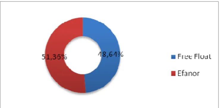
Sonae Industria’s shareholder structure can be seen in the chart below.

(23)

As we can see, the main shareholder of Sonae Indústria is Efanor Investimentos, SGPS with 51,36%, which is 100% owned by Mr. Belmiro de Azevedo.

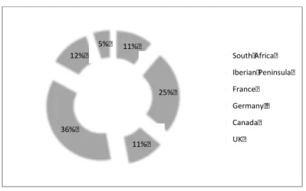
Currently, it is considered as a multinational firm, with production assets located in Portugal, Spain, Germany, France, United Kingdom (UK), South Africa and Canada. These locations are grouped in three main regions: Iberia, Central Europe that includes Germany, France and UK; the last one, Rest of the Worlds that encompasses Canada and South Africa. Internationalization expansion is crucial for the company, being the area with the largest proportion of sales Central Europe. The graph below, show us the total volume of sales per country.

Illustration 3.2: total volume of sales by country

Sonae Indústria 2010 annual report

Sonae Indústria is a wood panel producer with a broad product range that is based in three main categories of rawboards:

• Particleboard (PB): Engineered wood products made from wood particles (wood chips, sawmill, among others) that together with a suitable binder are pressed and extruded.

11% 25% 11% 36% 12% 5% South Africa Iberian Peninsula France Germany Canada UK

(24)

• Medium-density fibreboard (MDF): Engineered wood product manufactured by breaking down softwood (wood from conifers, e.g. pine and spruce) into wood fibres and mixing it with wax and resin.

• Oriented strand board (OSB): Engineered wood product produced by layering stands of wood in specific orientations. Strands of timber are resin-coated, then lain in layers, with the grain in each layer being oriented differently to maximise strengths and stability. The material is then cured under conditions of extreme heat and pressure, creating a dense, very string, dimensionally stable, durable engineered panel.

Illustration 3.3: total volume of sales by product

Sonae Indústria 2010 annual report

The Group is able to offer a wide range of wood-panel based products with main applications in the residential and commercial construction, office and home furniture, coverings and decoration. Downstream products are higher value added and a source of differentiation. Downstream products are transformed in higher value added and a source of differentiation. Over 90% of its capacity assigned to the manufacture of Particleboards (PB) and medium density fibreboards (MDF).

21% 17% 1% 8% 29% 9% 5% 2% 8% PB MDF HB OSB MF CTS TG Flooring Orhers

(25)

3.2 – Overview of wood panels industry

During the last decades, the wood panels industry has recorded significant growth rate. The industry took advantage of technological innovation in order to increase the use of its products in construction and furniture. The flexibility of use and the advantage of structured wood panels in home building have been a strong marketing tool, with the majority of people being familiarized with terms like MDF.

Nowadays, the wood panels industry has a global installed capacity of c. 1000mn m3/year.

Illustration 3.4: World Installed Capacity (c. 100mn m3)

Source: Euwid

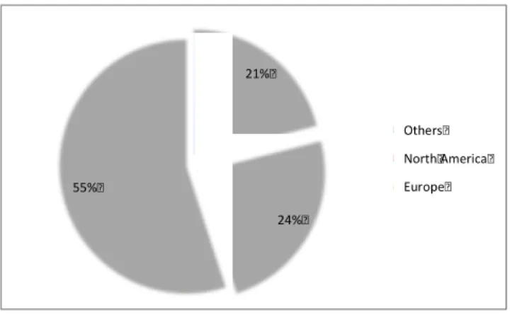
As wee can see, the main markets are Europe and North America but are also the more mature ones. However, due to the most dynamic growth registered in emerging economies such as Latin American and Eastern Europe (mainly Russia), they have been becoming the focus of attention from industry players. (Please refer to appendix 3)

The wood panels industry is a sector has a high sensitive to shift in demand and supply operating. There are two main factors that can explain: the business of wood panels is leveraged on the economic cycle and, on the other hand, market structure that explain the main difference among regions. Consequently, sometimes companies faced

21% 24% 55% Others North America Europe

(26)

Over the past years, the competition in this sector has been high. It is very fragmented market with some players at with low pricing power, except in some regions. Only natural wood, that presenting adaptation for specific client’s needs, appears as direct substitute product. Therefore, there are not significant threat concerns on substitutes products once wood derivatives products offer the best and efficient solution for its consumption target at lower price. The threat of new entrants is medium once it is necessary to reach economics of scales, several lawyers to follow, high initial investments and solid know-how (Please see to appendix 4).

In the last years, the price of wood panels have shown an increasing trend, namely in Europe, where the application of Kyoto principles has some influence through increased demand for recycled wood (which is one of main input in wood panels) from biomass energy producers. We can compare with pulp and paper industry that is another intensive wood consumer that must be considered in the price cycle wood. Difference in forest management policies among region also influences strongly the volatility of these prices and availability. In South Africa, wood panel price volatilities tend to be normalized with the implementation of new policies for forest development and maintenance.

It is important to refer that the wood panel market is mainly local, mostly due to high weighted of transport costs versus production costs. Therefore, producers tend to locate production line near their target market. In the cases where there are discrepancies between supply and demand in distant markets, the company practices a more expensive price in order to try to cover this “extra cost”. In that sense, the wood panels industry is normally seen not as a global but rather as multi-regional.

At the cost side, the price of raw materials and chemicals as the main concerns, the price of raw boards has been increasing, especially due to rising demand from petition industry (namely pulp and biomass) as well as it may be strongly affected by energies prices, some chemicals costs and wood price variations.

(27)

In relation to chemical costs, these are mostly related to urea (50%), methanol (35%) and other chemicals as well as water (15%). It is important take into account that the price of raw materials described before, after the slump from the 2008 they have been registering a slight growths.

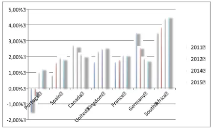
In what concerns of demand, the wood panel industry has a high correlation with GDP growth given that it reflects on available income of households (GDP macroeconomic expectations can be seen in appendix 5). The reason why the locations of Sonae Indústria’s plants are projected against the estimates of GDP growth is because wood panel revenues are significant correlated with construction activity, which is strongly affected by the economic performance on each country.

Illustration 3.5: Macroeconomic Estimates, GDP per country

In the future, changes in the technology may force producers to capacity replacements that otherwise would not need to occur. The last one occurred in the 90’s. All in all, the industry is becoming more capital intensive, given the company’s dimension and investment capacity.

Vertical integration through investments in downstream capacity protects profitability -2,00% -1,00% 0,00% 1,00% 2,00% 3,00% 4,00% 5,00% Port ugal Spai n Cana da Uni ted King dom Fran ce Germ any Sout h Af rica 2011 2012 2014 2015

(28)

The last but not the least, the current macroeconomic situation economic in Europe affects the business model of this industry.

3.3 – Impact of Economic Downturn

The global wood panel industry has faced complicated years due to the impact of recent Euro Sovereign crisis. Furthermore, key players in this sector have been adjusting their production levels face demand shortage.

Based on macroeconomic data, analysts stated that this data evidence better results than expected for the consensus. An example of this is Industrial confidence show us that it has been returned to pre-crisis levels. Employment rate and household confidence continues with a slow growth in countries with advanced economies but expanding in emerging markets, reflecting subdued employment.

There are other factors that may have had impact in the drop wood panels sales in G7 countries. These factors are mainly lack of credit availability, increases in oil prices, environmental issues and governments. The fits one helped, it was more contributed for decline in wood panels sales around the world.

Therefore, Sonae Indústria has been adjusted their business models according to the Financial and economic crisis.

3.4 – Sonae Indústria’s strategy

As already mentioned, Sonae Indústria is one of the largest wood panel’s players in the world, with a high leverage on innovation and operational efficiency not discarding the aim of growing supported by a strong balance sheet.

(29)

Sonae Indústria’s strategic goal guideline is to increase profitability in the market in which it operates. Top line growth per se is meaningless without the generation of a sustainable margin that is ultimately the main driver behind value creation; this goal is not only desirable but also utterly necessary.

An important part of the risk and opportunities of Sonae Indústria lies in the possible market structure changes that may occur locally. The degree of concentration in the different local markets determines broadly the profitability of each local business model. Some products show for higher margins (like OBS) than others (like particleboards), but it is the local market structure that determines and eventually offsets differences in profitability between production lines. This explains mainly why the French lines have been less profitability and partially why the South African have until recently been extremely profitable. The global expansion strategy allows for the some international diversification of local risks. The acquisition of a competitor has recently influenced the market structure in Central Europe. Therefore, increase profitability and improve competitiveness in Central Europe.

Taken into account all the issues discussed early, Sonae Industry’s management have been thinking in selling its plan in Russia since nature of the market is complex; they also will expect to sell of non-core assets, as is the case of Lure’s plant in France. On the other hand, the company keeps in mind the expansion in the US East Coast but the economic situation put the plan in stand-by. They also will expect

This company thinks that a good strategy would be to increase its exposure in Africa due to a five main issues:

I. Demand potential for wood panels products that should be supported by powerful macro conditions, accelerated spending on infrastructures and an undeveloped housing and construction sectors. Moreover, the Angolan government has recently announced that it plans to promote the development of the wood and furniture industries in the country.

(30)

III. Low competition. There is no wood panels production capacity in the country. Despite the potential human resources constrain, Sonae Indústria would benefit from a first-mover position.

Overall, Sonae Indústria believes the entrance in new and emerging markets would match its medium-long term strategy, set the bases for an extended presence in Southern Africa, and enhances its growth and earnings profile.

During the crisis, Sonae Indústria’s short-term strategy is minimizing working capital being extremely selective in making investments and looking for the opportunities; create a strong P&L by reducing fixed costs and increasing plants efficiency.

(31)

4 - Sonae Indústria Valuation

In this section I will show the valuation of the company, taking into account the main valuation approaches that I analysed previously as well as the strategy of the company and evolution of wood panels industry.

Due to the fact that Sonae Indústia operates in three different geographical areas: Europe, Africa and North of America, my initial aim was to do my valuation through Sum-of-the-Parts (STOP) by markets. However, the company did not provide all information that I needed to use this type of approach, consequently I chose a free cash flow to the firm WACC-based and the relative valuation based on the available information.

I will project cash flow from 2011 to until 2016, considering an explicit period of five years once it is the expected time that the Sonae Indústria will take to obtain stable annual cash flows. The terminal value will compute based on the last expected cash flow and I will assume an annual growth of 2%. This assumption of annual rate is consistent with the growth of geographies where company operates (that is in mature phases of lifecycle (except Africa that it is an emergent country but presents only 11% of sales).

In order to estimate the value of the expected cash flows, I will calculate their main drivers such as the company’s revenues, operating margin, Capex, depreciations and amortisations ad working capital.

Regarding relative valuation, I will start to define which is the most appropriate peer group for Sonae Indústria and then I will apply PER and EV/EBITDA multiples.

(32)

4.1 - Sonae Indústria Key Drivers

4.1.1 – Revenues

It is considered one of the main drivers; therefore it is important to understand all variables that can influence revenues. Sonae Indústria disclosed their revenue information according to four geographical areas: Iberia, Central Europe, South Africa and Canada. In order to reach a more accurate forecast of the revenues in each area for Sonae Indústria, we need to compute separately the production and price.

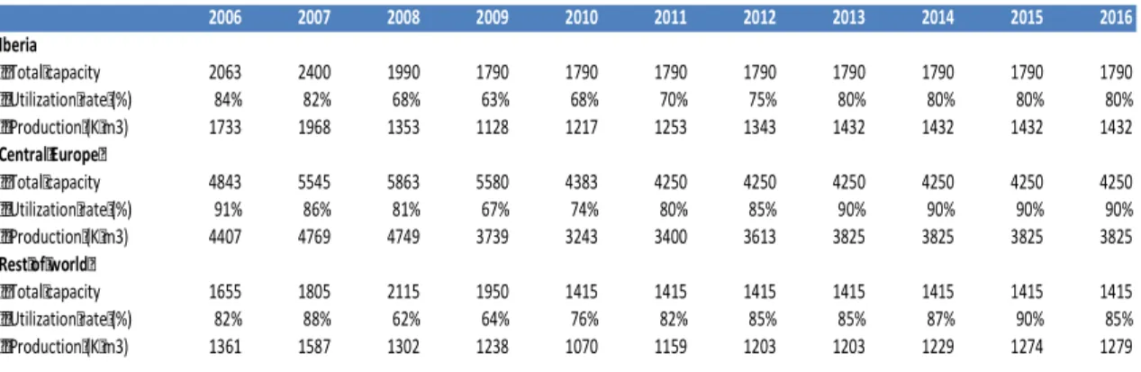
A) Production

Sonae Indústria is one of the largest global players of wood based panels in Europe and worldwide with installed capacity of 7455 m3. This company benefits from very high levels of capacity utilization rate, however, in recent years it has been faced over capacity and adjusting its production structure to market conditions. Thus, it has been

stated to close old and less efficient capacities and undertaking productivity improvements across its facilities.

Illustration 4.1 – Total Production per region

Source: Company data

Capacity projections are based on Sonae Indústria estimates, which, according to their expansion plan in medium term, this company doesn’t expect to have more capacity

2006 2007 2008 2009 2010 2011 2012 2013 2014 2015 2016 Iberia Total capacity 2063 2400 1990 1790 1790 1790 1790 1790 1790 1790 1790 Utilization rate (%) 84% 82% 68% 63% 68% 70% 75% 80% 80% 80% 80% Production (K m3) 1733 1968 1353 1128 1217 1253 1343 1432 1432 1432 1432 Central Europe Total capacity 4843 5545 5863 5580 4383 4250 4250 4250 4250 4250 4250 Utilization rate (%) 91% 86% 81% 67% 74% 80% 85% 90% 90% 90% 90% Production (K m3) 4407 4769 4749 3739 3243 3400 3613 3825 3825 3825 3825 Rest of world Total capacity 1655 1805 2115 1950 1415 1415 1415 1415 1415 1415 1415 Utilization rate (%) 82% 88% 62% 64% 76% 82% 85% 85% 87% 90% 85% Production (K m3) 1361 1587 1302 1238 1070 1159 1203 1203 1229 1274 1279

(33)

reductions. In relation to the current installed capacity once they consider that the “business is adjusted to the current macro economic conditions faced in the last two years”. However, the management recognizes that capacity can experience decreases in capacity in Iberia and Central Europe due to the low demand if the macroeconomic conditions worsen. In my projections of utilization rate I didn’t consider any capacity reductions (For more details per region, please refer to appendix 6).

Looking at the past, we can see that Sonae Indústria decreased their utilization rate between 2008 and 2009 due to the rebalance between demand and supply.

B) Price

To estimate the prices (per cubic meter), the first process is to look at the historical evolution of prices in the different geographic areas. These historical prices were computed based on total sales in each region divided by the total production per cubic meter.

One of the main difficulties was to get the data. As Sonae Indústria didn’t provide enough information that I needed to compute the price for three different types of products for each specific country, the first assumption is that the three types of wood panels have the same price.

The best way to compute the future price was to use the inflation rate. As the company disclosed only the sales of the different countries that operate in Euros i.e. as the price was already converted from the local currency to euro, the other assumption is that the future price is based on the inflation rate in Europe (Please refer to appendix 7). In other words, the future prices of the products of the different geographies grow at inflation rate in Europe.

(34)

Illustration 4.2 – Price by geographical areas

C) Total volume

Once we analyse the historical data and forecast the main inputs that I discussed previously, such as capacity in the different areas geographic as well as the corresponding price, we have all the information to compute the expected volume of sales of the regions that Sonae Indústria operates:

I – The total production obtained at the end of each period for each area was obtained by multiplying the utilization rate by total capacity per m3.

II – In order to support my assumption of price, I looked at the expected annual average consumer price (Inflation) for the Euro zone in the next five years, according to published in the WEO of International Monetary Fund. Thus, futures prices grow at inflation in Euro zone.

III – Lastly, the total sales at the end of each period by region were obtained by multiplying the total production by future price. In order to obtain the sum-of-the – parts it is only the sum of total sales of each geographic area.

Illustration 4.3 – Total volume of revenues by area

Price (Eur/m3) 2006 2007 2008 2009 2010 2011 2012 2013 2014 2015 2016 Iberia 264,9 270,8 334,8 302,4 301,5 308,3 313,6 319,2 324,9 331,4 337,7 Central Europe 216,5 252,9 206,4 185,4 213,0 217,9 221,6 225,5 229,6 234,2 238,7 Rest of World 254,95 218,01 278,21 212,29 234,52 239,82 243,96 248,26 252,75 257,78 262,71 2006 2007 2008 2009 2010 2011 2012 2013 2014 2015 2016 Revenues (in M€) Iberia 459,0 533,0 453,0 341,0 367,0 386,3 421,1 457,1 465,3 474,6 483,7 Central Europe 954,0 1206,0 980,0 693,0 691,0 740,7 800,6 862,6 878,2 895,7 912,8 Rest of world 347,0 346,0 362,1 262,9 251,0 278,0 293,4 298,6 310,5 328,3 335,9 Internal sales -41,12 -18,03 -26,05 -14,02 -16,44 0 0 0 0 0 0 Total Revenues 1718,88 2066,97 1769,1 1282,9 1292,6 1405,0 1515,1 1618,3 1654,0 1698,5 1732,4

(35)

According to the table below, the major part of the total volume derives from Central Europe that represents around 51% of total sales but Iberia and Central Europe together represent approximately 80% of the total volume. It is important that there are two comparable markets that are in a similar position of life cycle: they are in the mature phases.

In the past, due to the depressed macro situation that Europe is facing, the business environment suffers from restrictions such as overcapacity and inefficient factories both in Central Europe and Iberia, the two main geographical areas. However, Sonae Indústria expects that the business environment to improve once, especially given the latest macroeconomic indicators that show a small recuperation in industrial production.

On the other hand, Canada and South Africa (included in “Rest of world”) are markets that were not affected by the economic crisis that Europe faced since 2008. Sonae Industria’s activity in South Africa should benefit from a solid macro environment (GDP estimated to grow 3,5% in 2011 and 3,8% in 2011) and a consolidated market structure. In the following years there’s an expected rise of sales in this region. In Canada, it is expected to continue to grow and increase its utilization rate although industry outlook remains constrained by a weak construction and housing sector.

4.1.2 – Operating Costs

After forecasting the sales, the next key step is to calculate the EBITDA margin, which are the revenues (gross profit) less the operating costs. As I mentioned before, not all the information is disclosed, therefore the cost composition is not possible to forecast by geographical segmentation in order to provide a more accurate valuation. Most of the estimated values were based on historical data and a few assumptions looking at industry expectations for the coming years.

(36)

the main operating costs are Cost of Goods Sold (COGS). Operating expenses can be divided in Cost of Goods Sold, Selling General and Administrative Expenses and Other Operating Expenses.

The Cost of Goods Sold (COGS) primarily includes all raw materials, namely chemicals and raw woods, which the firm needs for the transformation into woods panels. I assumed that all these costs vary according to sales and it would be constant equal to 46,4% of turnover, the average of the last three years. I considered the best way to estimate COGS once the company did not disclose the information by region.

External Suppliers and Services represent transportation costs, energy costs, among others. In the same line of though of COGS, I assumed for the following years a ratio of 26% of revenues based on the average of the last three years.

Regarding to the Staff Expenses, I analysed separately the two main inputs: the evolution of number of employees and average cost per employee. The first step was to compute cost per employee that was the result from the division of the total cost of this rubric by average of employee in this year. According to Sonae Indústria, they believe that the average number of employees remain constant in the next years in order to cut costs. On the other hand, the average cost per employee was affected by the expected inflation rate, in other words, to grow at inflation rate (please refer to appendix 7).

The item “Other operating costs” essentially includes expenses relating to factories operations and general overheads. I assumed an average of the last three years as a percentage of total sales. For the following years, I maintained constant a ratio of 1,1% of sales. In the appendix 8 can be seen OPEX.

(37)

4.1.3 – Depreciations and amortisations

In what concerns the depreciations and amortisations, the first stage was to analyse the historical values of tangible assets and intangible assets as well as depreciation and amortization for each year, respectively. Thus, I could understand the allocation of “costs” of each type of assets.

In order to compute depreciations, I assumed it as the percentage of the value of tangible assets at the beginning of this year. This percentage is based on data of 2010 and Sonae Indústria’s management will expected no changes in this topic in the next years. Regarding amortisations is the same line of thought.

In the following table, we have expected depreciations and amortisations for the next years based on historical values.

Illustration 4.4 – Depreciation and amortisation scheduled

Depreciations and Amotisations Tangible Asset % of total Taangible asset Intangible Asset % of Total Intangible asset 2011 2012 2013 2014 2015 2016 78,68 74,39 70,44 66,80 63,46 60,38 8,0% 8,0% 8,0% 8,0% 8,0% 8,0% 2,43 2,42 2,42 2,41 2,41 2,41 24,0% 24,0% 24,0% 24,0% 24,0% 24,0%

4.1.4 – Investment Policy

In relation to capital expenditures (CAPEX) in Sonae Indústria, the two mains items are expansion plan and investment policy in terms of tangible and intangible assets investments.

As I mentioned before, this firm faces a mature phase of life cycle and, in the last years it has been removed off their balance sheet all plant that were less efficient and made improvements across its facilities with the aim to resolve their structural problems related to overcapacity due to oscillations between demand and supply. Thus, in the last years, this company made some disposals with the aim to become a solid

(38)

company. According to management’s Sonae Indústria, they will not expect more disposals during my period of valuation. Therefore, I assumed zero for the future. Sonae Indústria’s annual investment will be near €28M based on historical values and company projections. This annual CAPEX is principally maintenance in order to cover the annual depreciation and as well the increases in efficiency of their plants.

Illustration 4.5 – CAPEX

Capex Tangible Asset Intangible Asset Total Capex 2011 2012 2013 2014 2015 2016 25,00 25,00 25,00 25,00 25,00 25,00 2,40 2,40 2,40 2,40 2,40 2,40 27,40 27,40 27,40 27,40 27,40 27,40

4.1.5 – Net Working Capital

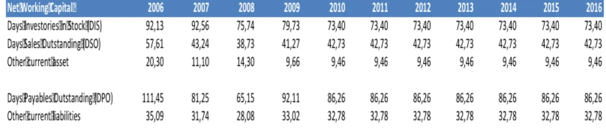
According to Sonae Indústria’s disclosed results, I was able to have all necessary information to calculate net working capital. In the firm’s annual reports we have the following items of the operational working capital:

• Receivables: include trade receivables, states and other public entities and other current receivables.

• Payables: trade payables and other current payables.

• Inventories: includes all necessary raw materials and consumables as well as products in process and finished goods for sales.

In order to compute the working capital for the next years, I started by calculating the historical days receivables, days’ payables and the inventory period. For the following years, I based my calculations on the historical data on 2010 once this year reflects the expected Sonae Indústria’s policy in term of net working capital. For more details, please refer to appendix 9.

(39)

Illustration 4.6 – Net Working Capital

4.1.6 – Taxes

Forecasting Sonae Industria’s taxes was a hard task since it is a multinational firm where each country has different ways to calculate income tax, as well as applying different taxes, which is regulated by the Government of the respective country. In some countries such as Germany, applying different taxes among the different states.

Besides these difficulties, there was another problem related to the tax credits. In the last three years, Sonae Indústria had a negative net income. When a company has a negative net income, it has the tax benefit. I tried to ask the company the countries it had a negative net income but due to competition issues, they did not provide information about fiscal activity in a consolidated way.

Consequently, some simplified assumptions were made. The first one, if Sonae Indústria has a positive net income, it has positive net income in all countries where it operates. Regardless to the tax system, I assumed that the tax rate didn’t differ from country to country. The last assumption in this issue was when the company had accumulated losses from the preceding years; it can be carried forward for the next years since it is expected that the firm will generate positive net operating income from now on. Therefore it can benefit from tax credits. Thus, in the following years when it generates positive operating results, instead of paying taxes, it can deduct

Net Working Capital 2006 2007 2008 2009 2010 2011 2012 2013 2014 2015 2016 Days Investories in Stock (DIS) 92,13 92,56 75,74 79,73 73,40 73,40 73,40 73,40 73,40 73,40 73,40 Days Sales Outstanding (DSO) 57,61 43,24 38,73 41,27 42,73 42,73 42,73 42,73 42,73 42,73 42,73 Other current asset 20,30 11,10 14,30 9,66 9,46 9,46 9,46 9,46 9,46 9,46 9,46 Days Payables Outstanding (DPO) 111,45 81,25 65,15 92,11 86,26 86,26 86,26 86,26 86,26 86,26 86,26 Other current liabilities 35,09 31,74 28,08 33,02 32,78 32,78 32,78 32,78 32,78 32,78 32,78

(40)

4.1.7 – Other Items

Concerning to cash and cash equivalents, it was assumed as a percentage of sales based on average of the last three years and I considered that this ratio would maintain constant in the next years. Furthermore, I assumed that cash and cash equivalents was totally non-operating. Thus, I will use cash and cash equivalents to amortize debt; this indicates that for the calculation of net debt value, I need subtract the cash balance, assuming it as excess cash.

According to Sonae Industria’s information, they do not expect changes in ownership structure of the group. Therefore, I did not consider deviations of minority interests.

Regarding to dividend issues, this company has not been paying dividends. However, Sonae Indústria will be expected to continue not paying dividends on its stock since the current economic conditions are not the best.

4.2 – Debt

Debt was one of the most difficult things to estimate since the company did not provide all information that I needed to calculate them. Consequently, some simplified

assumptions were made. The first one, it was assumed that debt in book values it is the same to its market values. Besides this, the debt in the balance sheet would change concerning to the financing needs of firm.

Regarding to predict debt, the first thing was to understand the composition of company’s debt. Sonae Industry’s debt is combined by long-term and short-term debt with weight of 77% and 23%, respectively. In relation to long-term debt includes commercial paper, bank loans, non-convertibles debentures as well as obligations under finance leases while short-term debt encompasses bank loans and obligations under finance leases.

(41)

In what concerns to existing long term debt, since information was shortage, it was assumed that this type of debt would be repaid considering maturity on average of three-year. On other hand, existing short-term debt, it has maturity on average half-year; it would be totally paid until the end of each year.

For the following years, the company could not provide information about the refinancing at this point. Nevertheless, Sonae Indústria recommended that both percentages of long-term and short-term debt could continue the same in the future once, between the two financing sources, they prefer long-term debt. In the appendix 10, we can find all details about debt and repayments.

4.3 – Valuation assumptions

According to reasons already stated before, I chose the FCFF (free cash flow to the firm WAAC-based) to value Sonae Indústria. In order to correctly discount the FCFF, I used CAPM formula and several assumptions were made implicit in the model.

4.3.1 – Risk free rate

The risk free rate used was Yield on the German’s 10-years treasury bond of 3,50%. Although Sonae Indústria operates in different countries, more than 65% of its business is made in Europe.

4.3.2 – Market Risk Premium (MRP)

In relation to Market Risk Premium, I considered separately the two effects: market premium and specific country risk premium. According to Damodaran source, I assumed a market premium of 5,0% for developing countries. Although, due to actual circumstances in Euro zone sovereign crisis, an additional spread of 2,5% it was considered, as the company operates in several companies affected by this crisis. Therefore, MRP is the sum of these two elements that is equal to 7,5%.

(42)

4.3.3 - Beta

Regarding to Beta, I used Damodaran’s estimative for Paper and Forest Product unlevered beta is equal to 0,95.

Illustration 4.7 – Steps to compute levered beta

2011 2012 2013 2014 2015 2016 Beta Industry Unlevered Beta 0,95 0,95 0,95 0,95 0,95 0,95 Levered Beta 1,351 1,310 1,250 1,201 1,153 1,105 Tax rate 29% 29% 29% 29% 29% 29% Debt/Asset 50,1% 48,5% 46,0% 43,8% 41,5% 39,0% Equity/Asset 49,9% 51,5% 54,0% 56,2% 58,5% 61,0% Capital Structre 100% 94% 85% 78% 71% 64%

4.3.4 – Cost of equity

Once estimated all drivers found above, the CAPM formula was applied with the purpose to obtain the Cost of Equity. In Sonae Industria’s case, the Cost of Equity was equal to 13,63% in 2011. Please refer to appendix 11 in order to see the steps for compute the cost of equity.

4.3.5 – Weighted Average Cost of Capital

Now that all assumptions have been explained, we can calculate the cost of capital. In order to assure a more accurate and real valuation of Sonae Indústria, I decided to compute the Cost of Capital for each individual period. This assumption is in line with the fact that the capital structure of this company has been changed every year but not suffer significant alterations. As the management of Sonae Indústria stated “We have a specific target of capital structure of E/V is equal to 70%. Due to the macroeconomic conditions it is quite impossible to reach this target in medium term. However, our management has been working over the time for decrease our debt’s level”.

(43)

The table below show us the WACC for each year as well as the different components of them.

Illustration 4.8 – Cost of Capital

2011 2012 2013 2014 2015 2016 Beta Industry Unlevered Beta 0,95 0,95 0,95 0,95 0,95 0,95 Levered Beta 1,351 1,310 1,250 1,201 1,153 1,105 Tax rate 29% 29% 29% 29% 29% 29% Risk-free Rate 3,50% 3,50% 3,50% 3,50% 3,50% 3,50% Equity Risk Premium 5,00% 5,00% 5,00% 5,00% 5,00% 5,00% Country Risk Premium 2,50% 2,50% 2,50% 2,50% 2,50% 2,50% Market Risk Premium 7,50% 7,50% 7,50% 7,50% 7,50% 7,50% Cost of Debt 4,93% 6,56% 7,46% 8,09% 8,77% 9,07% After tax cost of Debt 3,50% 4,66% 5,30% 5,74% 6,23% 6,44% Cost of Equity 13,63% 13,32% 12,88% 12,51% 12,14% 11,79% Debt/Asset 50,1% 48,5% 46,0% 43,8% 41,5% 39,0% Equity/Asset 49,9% 51,5% 54,0% 56,2% 58,5% 61,0% Capital Structre 100% 94% 85% 78% 71% 64% WACC 8,56% 9,12% 9,39% 9,54% 9,69% 9,70% WACC in perpetty 7,70%

4.3.6 – Enterprise and Equity Value using DCF

Finally, it was possible to reach final value of firm (Enterprise Value) after to added up all things considered previously. This means, the enterprise value (EV) computed by WACC method is € 128,41 million Euros.

After to get the firm value, it was necessary to make some adjustments in order to obtain price per share. These adjustments were related to net debt, minorities’ interests and financial investments. Due to the reasons that it was explained before, it was necessary to deduct excess cash from firm value.

(44)

Illustration 4.9 – Steps necessary for compute the Price per Share

2010 2011 2012 2013 2014 2015 2016 EBIT -25,90 20,09 47,48 72,64 80,53 89,74 96,13 Taxes 7,51 -5,83 -13,77 -21,07 -23,35 -26,02 -27,88 Depreciations 95,35 81,11 76,81 72,85 69,22 65,87 62,79 Changes in NWC -0,48 2,19 4,06 3,80 1,32 1,64 1,25 Capex 20,26 -27,40 -27,40 -27,40 -27,40 -27,40 -27,40 FCFF 96,73 70,16 87,17 100,83 100,31 103,82 104,89 Discount Factor 92,12% 84,42% 77,17% 70,45% 64,23% 58,55% PV FCFF 64,63 73,59 77,82 70,67 66,68 61,41 Sum PV FCFF 414,79 Terminal Value 813,05 EV 1227,84 Minority Interests 0,98 Net debt 717,97 Equity value 508,88 # shares 140 Price in Euros 3,63

4.4 – Relative Valuation

As was mentioned in Literature Review section, relative valuation is useful way to do comparisons with the market and it is used as a support to a discounted cash flow models.

In order to value Sonae Indústria through relative valuation, the first consideration was to define the peer group to be used. It was a difficult task due to the fact that the company has big range of peers group. Therefore, Sonae Industria’s peer group is publicly-traded companies and refers only the players in wood panels based industry with same business activities, growth and similar levels of risk. The below table presents the peer group of Sonae Indústria for 2011 and 2012:

(45)

Illustration 4.10 – Data of comparable companies and multiples

2011E 2012E 2011E 2012E

Pfleiderer 127,0 24,1 33,7 6,5 4,8 Louisiana Pacific 762,7 29,1 27,4 8,3 4,5 Norbord 385,7 72,8 12 9,8 4,6 Duratex 2916,0 14,4 12,7 7,9 6,6 Weyerhaeuser 8334,0 44,2 25,4 12,2 10,8 Temple Inland 1746,0 16,7 10,4 5,8 4,3 Sonae Industria 214,2 34,0 20,5 10,1 8,5 Average 2378,6 33,6 20,3 8,4 5,9 P/E EV/EBITDA Market Cap (€ mn)

Source: Bloomerg and company’s annual report 2010

The methodology used to defining the peer group was weighted average of the peer’s comparable multiples. In relation to multiples, initially the multiples chosen to calculate the value of firm were EV/EBITDA and price-earnings multiple (PER) for compute value of equity.

As I mentioned in Literature Review, EV/EBITDA is difficult to manipulated by changes in the capital structure and depreciation policy. In order to understand better this point, in the table below it is illustrated the bull case and bear case, with 1,0x de deviation from base case.

As Sonae Indústria will expect to have negative earnings in 2011 and 2012, it is impossible to calculate the value of company using PER multiple.

(46)

Illustration 4.11 – Share price using multiples

Bear Case Base Case Bull Case

Target EV/EBITDA 9,06 10,06 11,06 EBITDA 2011 101,20 101,20 101,20 Target EV 917,21 1018,41 1119,61 Net debt (2010) 717,97 717,97 717,97 Minorities 0,98 0,98 0,98 Equity 198,25 299,45 400,65 Number of Shares 140,00 140,00 140,00 Price per Share 1,42 2,14 2,86

Once to reach the equity value of firm through EV/EBITDA multiple, it is possible to obtain a price per share after I have done some adjustments, as can be seen in the illustration 4.11. All in all, in the base case of EV/EBITDA multiple, Sonae Indústria has a price per share of € 2,14.

This method is not the most appropriated to compute a price target due to considerable difference between the peer’s performance.

(47)

5 -Valuation Comparison

In this section will be compare my valuation of Sonae Indústria with the report of Millenium Investment Banking (MIB). Equity analyst João Mateus launched this report on the 12th May 2011, with the price target of € 3,30, which represents 162% above my valuation. In order to identify the main factors that explain the difference, I started to investigate their assumptions. The most important are:

Valuation method: in my thesis, I used DCF WACC-based method since capital structure is expect to change in order to reach the target level but without significantly alterations over the years. Net Debt of 2010 is used to calculate the end-2010 price target. The analyst of MIB uses the sum-of-the-part by regions and also it is use Net Debt at the end-2010.

Discount factor: I applied different WACC over the years while investment bank assume the same WACC during the explicit period. It is important mentioned as MIB uses sum-of-the-part for each area that Sonae Indústria operates, their assumptions regarding the market risk premium and the beta is for each specific region. Thus, it is possible that the discounted factor vary form my own valuation. The table below included all assumptions was made for investment bank in relation to WACC components:

Illustration 5.1 – Components of Cost of Capital estimated by MIB

Risk-free CRP + ERP Levered beta Cost of debt Cost of Equity WACC Growth WACC - g perpetty

Iberia 3,25% 8,50% 156,00% 8,00% 16,55% 12,28% 2,00% 10,28%

Central Europe 3,25% 5,00% 154,00% 8,00% 10,95% 8,81% 2,00% 6,81%

Canada 3,25% 6,50% 151,00% 8,00% 10,78% 8,55% 2,00% 6,55%

South Africa 3,25% 5,00% 161,00% 8,00% 13,72% 10,78% 2,00% 8,79%

Sonae Indústria : equity valuation