Load Balancing for Constraint Solving with
GPUs
Pedro Roque, Vasco Pedro, and Salvador Abreu
Universidade de ´Evora/LISP
[email protected], [email protected], [email protected]
Abstract. Solving a complex Constraint Satisfaction Problem (CSP) is a computationally hard task which may require a considerable amount of time. Parallelism has been applied successfully to the job and there are already many applications capable of harnessing the parallel power of modern CPUs to speed up the solving process.
Current Graphics Processing Units (GPUs), containing from a few hun-dred to a few thousand cores, possess a level of parallelism that surpasses that of CPUs and there are much less applications capable of solving CSPs on GPUs, leaving space for further improvement.
This paper describes work in progress in the solving of CSPs on GPUs, CPUs and other devices, such as Intel Many Integrated Cores (MICs), in parallel. It presents the gains obtained when applying more devices to solve some problems and the main challenges that must be faced when using devices with as different architectures as CPUs and GPUs, with a greater focus on how to effectively achieve good load balancing between such heterogeneous devices.
Keywords: Constraint solving, Paralellism, GPU, Heterogeneous sys-tems
1
Introduction
Some real life problems such as scheduling, resource allocation and route def-inition, and also some academic problems like the Costas Array [12] and the n-Queens1, can be modelled as Constraint Satisfaction Problems (CSPs).
Solving a complex CSP may require a considerable amount of time. As such, parallelism has been applied to speed up the solving process, based on the insight that a CSP could be solved faster by splitting it into multiple sub-problems that could be solved independently on different threads spread over multiple cores, de-vices or even machines. Many applications, as the ones presented in [3,10,11,16], use this method for solving CSPs on multi-core CPUs.
Current GPUs have much more parallel processing power than current CPUs, being capable of running hundreds, or even thousands of threads simultane-ously [8], which makes them attractive to perform parallel tasks, like solving
1
CSPs. Some authors, such as Arbelaez and Codognet [1], Campeotto et al. [2], and Jenkins et al. [5] found that GPUs can be more effective than CPUs in large tasks that can be highly parallelizable. Nevertheless, programming an ap-plication capable of using all that parallel processing power is a great challenge, mostly due to the complex hardware architecture of GPUs.
This paper describes the main features of the CSP solver that we are develop-ing, named Parallel Heterogeneous Architecture Constraint Toolkit (PHACT), with special emphasis on the load-balancing issues. PHACT is already capable of solving CSPs in parallel on GPUs, CPUs and Intel Many Integrated Cores (MICs), and we present the results achieved when solving the n-Queens and the Costas Array problems on multiple combinations of devices, showing that using heterogeneous devices for solving the same CSPs can lead to a good performance boost.
Nevertheless, some problems arise when using simultaneously devices with such different architectures as CPUs and GPUs. Those problems and the tech-niques used for overcoming them are also presented.
In the next section the CSPs main concepts are described. Section 3 presents some works done by other authors on this subject. In Section 4 the main features of the solver are described. The results and discussion are presented in Section 5, and the conclusion and future work are placed in Section 6.
2
CSPs concepts
A CSP can be defined as a set of variables with defined domains, and a set of constraints between the values of those variables. The solution of a CSP is the assignment of one value from the respective domain to each one of the variables, ensuring that all constraints are met.
Definition 1. Formally a CSP is defined as a triple P = hX, D, Ci, where: – X = hx1, x2, ..., xni is an n-tuple of variables;
– D = hD1, D2, ..., Dni is an n-tuple of finite domains, where Di is the domain
of variable xi;
– C = {C1, C2, ..., Cm} is a set of relations between variables in X, designated
as constraints.
A CSP solution is an n-tuple A = ha1, a2, ..., ani where ai ∈ Di is the value
assigned to variable xi and all the constraints Cj are met.
For example, the n-Queens problem consists in placing n queens on a n × n chess board such that no queen attacks another one. It can be modelled as a CSP with n variables and with the constraints stating that each board row, column or diagonal cannot contain more than one queen. Each variable maps to a different board column and each variable domain contains the integers that correspond to the board rows where each queen may be placed. The solution to this CSP will be the assignment of a value of the respective domains to each of the n variables while all the constraints are met.
The methods for solving CSPs can be categorized as incomplete or complete. Incomplete solvers do not guarantee that an existing solution will be found, being mostly used for optimization problems and for large problems that would take too much time to fully explore. Incomplete search is beyond the scope of this paper and will not be discussed here.
On the contrary, complete methods guarantee that if a solution exists, it will be found. Finding solutions to a CSP in a complete solver is usually done with backtracking and iterating two stages:
– Labelling - Selecting and assigning a value to a variable. This value must belong to the variable domain;
– Constraint propagation and consistency check - Propagates the assignment of a value to one variable to the domains of other variables. This process aims to reduce the number of elements in those domains and to check if any constraint is no longer satisfiable, which would mean that the set of assigned values is not part of a solution.
3
Related work
Searching for CSP solutions in a backtracking approach can be represented in the form of a search tree. To take advantage of parallelism this search tree is split into multiple subtrees and each one of them is explored in a different thread that may be running on a different core, device or machine.
This is the approach generally taken by authors that develop constraint solvers which will run on single or distributed multi-core CPUs [3,10,11,16].
Pedro developed a CSP solver named Parallel Complete Constraint Solver (PaCCS) capable of running from a single core CPU to multiple multi-core CPUs in a distributed system [10]. Using work stealing for distributing the work among the threads and the Message Passing Interface (MPI) to allow communication between them, this author achieved in average, almost linear speedups for most of the problems solved.
R´egin et al. implemented an interface responsible for decomposing an initial problem into multiple sub-problems filtering out those found to be inconsis-tent [15]. After generating the sub-problems it creates multiple threads, each one corresponding to an execution of a solver (e.g., Gecode [17]), to which a sub-problem is sent at a time for exploration.
For some optimization and search problems, where the full search space is explored, these authors achieved average gains of 13.8 and 7.7 against a sequen-tial version, when using Gecode through their interface or just Gecode, respec-tively [15]. On their trials, the best results were achieved when decomposing the initial problem into 30 sub-problems per thread and 40 threads on a machine with 40 CPU cores.
While solving CSPs through parallelization has been a subject of research for decades, the usage of GPUs for that purpose is a recent area, and as such there aren’t many published reports of related work. To our knowledge, there are only
two published papers related with constraint solving on GPUs [1,2]. From these two, only Campeotto et al. presented a complete solver [2].
Campeotto et al. developed a CSP solver with Nvidia’s Compute Unified Device Architecture (CUDA), capable of using simultaneously a CPU and an Nvidia GPU to solve CSPs [2]. On the GPU, this solver implements an approach different from the one mentioned before, namely, instead of splitting the search tree over multiple threads, it splits each constraint propagation over multiple threads.
Campeotto et al. exploit parallelism in three levels:
– The constraints relating many variables are predefined to be propagated in the GPU, while the remaining constraints are filtered sequentially by the CPU. To balance the load between the CPU and the GPU, a preprocessing step is done to determine which propagations should be done on each device, taking into account the estimated number of global memory accesses that the GPU would require for each propagation.
– On the GPU, the propagation and consistency check for each constraint is assigned to one or more blocks of threads according to the number of variables involved;
– The domain of each variable is filtered by a different thread.
One of the main bottlenecks when working with GPUs is the low bandwidth transfer rate between host and device, so the number of transfers and the amount of data transferred must be minimized. Campeotto et al. reduced the data trans-fer to a minimum by transtrans-ferring to the GPU only the domains of the variables that weren’t labelled yet and the events generated during the last propagation. The events allow classifying the last action applied to that domain. For exam-ple, they may indicate that an element was removed and this allows applying the appropriate propagator.
Again, to reduce data transfers, the domain of each CSP variable is repre-sented as a 32-bit bitmap, and three other variables are used for storing the domain bounds and the last event associated with that domain.
All the data transfers between host and device are made asynchronously, and only after the CPU has finished his sequential propagation both GPU and CPU will be synchronized.
Campeotto et al. obtained speedups up to 6.61 with problems like the Lang-ford Problem and some real problems such as the modified Renault problem [6], when comparing a sequential execution on a CPU with the hybrid CPU/GPU version. The best results were obtained with the largest instances of problems, showing that the usage of GPUs is best for the biggest CSPs.
4
Multi-device implementation
One of the biggest challenges when developing an application capable of running on different types of devices like GPUs, CPUs and MICs, is achieving the best performance on all these devices.
From among these devices, the most challenging ones for developing a solver are the GPUs due to their complex memory hierarchy and to their hardware architecture in general [5]. For example, the Nvidia GeForce GTX 980 memory is split physically and/or virtually in four different types that have their benefits and limitations and should be used accordingly, or the application performance will suffer greatly [9].
This GPU has 16 Streaming Multiprocessors (SM) with 128 CUDA cores each, making a total of 2048 CUDA cores. Nevertheless, each SM is only ca-pable of executing simultaneously 32 threads (using only 32 CUDA cores at the same time), which means that this GPU is capable of running 512 threads simultaneously [9].
This is a huge level of parallelism, but most of the GPUs are built mainly for graphics processing which normally deals with lots of data and only a few different operations on that data, making general purpose applications which usually have lots of different operations and fewer data, much less effective on this type of hardware [5].
Currently there are two main programming languages that may be used for general purpose programming of GPUs: CUDA and OpenCL [4]. CUDA is the Nvidia GPU programming language and is only compatible with Nvidia GPUs. On the contrary, OpenCL is compatible with GPUs, CPUs, MICs and other devices from multiple vendors. As we want a CSP solver capable of running on multiple types of devices and from different vendors this was the chosen programming language.
The OpenCL programming language has a few important concepts that must be described in order to understand the remaining contents of this paper:
– Compute unit - In Nvidia GPUs each SM is a compute unit. AMD GPUs have their own components called Compute Units that match this definition. For CPUs and MICs, the number of available compute units is normally equal to or higher than the number of threads that the device can execute simultaneously [7];
– Kernel - This is the code that will be executed in each thread;
– Work-item - This corresponds to a different instance of the kernel (thread) that may be executed in parallel;
– Work-group - Each work-group is composed of one or more work-items that will be executed on the same compute unit. All work-groups for one kernel have the same number of work-items;
– Host - CPU where the application responsible for initializing the kernels is executed;
– Device - CPU, GPU, MIC or other device where the kernels are executed. In [12] and [13] we presented multiple trials with a previous version of PHACT, that was only capable of running on current GPUs. Afterwards, in [14] we described the new features that allowed PHACT to run on GPUs, CPUs and MICs, but only on one device at a time. Currently, PHACT is already capable of splitting work between multiple CPUs, GPUs and MICs located on the same
machine. So far, PHACT was only tested on some CPUs, GPUs and MICs, but it was implemented to run on any device compatible with OpenCL.
The main features of the solver are:
– Each CSP variable domain is represented as a bitmap of 32, 64, or multiples of 64 bits, according to the maximum size of the variables domains; – The initial search space is split into multiple sub-search spaces that are
grouped together and sent to the devices in blocks;
– Each device will explore multiple sub-search spaces simultaneously;
– Each work-item will do labelling, propagation and backtracking on a sub-search space at a time;
– If only one solution is sought, the kernel finishes when a work-item finds a solution and the solution is then transferred back to the host;
– If all solutions must be found the kernel finishes when all sub-search spaces have been explored, and the number of solutions is then transferred back to the host;
– The variable to label can be selected using one of the following heuristics: • The leftmost variable [13];
• The variable that has less values in its domain; • The variable that is more constrained.
Distributing the search spaces
From CPUs, MICs and GPUs, the most challenging ones for programming PHACT are the GPUs. The usage of this type of devices implies two main challenges:
– The size and number of transfers between host and device must be reduced as much as possible, because these are very expensive operations;
– While executing a kernel on a GPU, it is not possible to programmatically stop or pause that kernel.
These two challenges made us look for new techniques to distribute the work between devices. For example, R´egin et al. place all the initially generated sub-search spaces on a queue, from where all the workers pick one at a time to explore, until all are explored [15]. For GPUs, this technique would be problem-atic, because this would lead to a huge number of transfers between host and device, resulting in a great performance loss.
Some tasks may overlap GPU computation with CPU-GPU communication to reduce the costs of moving data between these devices [18]. This technique requires that the execution time and/or the device mapped-memory accesses of the task which will be executed on the GPU are somewhat predictable, which is not the case when solving a CSP, making this technique unsuitable to be applied in PHACT.
Before executing the kernel, we must send as many sub-search spaces as possible to the GPU, to reduce the number of transfers needed. The problem is that the load must be balanced between all the devices (CPUs, GPUs and
MICs) and if we send too many sub-search spaces to a slower device it may finish exploring them way after the faster devices have explored all the remaining sub-spaces. As it stands, there is no way to programmatically stop a kernel to redistribute the remaining sub-search spaces between devices.
Attending to all these challenges a new technique was implemented, to min-imize the number of transfers between devices and host while trying to make all the devices finish their exploration around the same time. This technique uses two metrics:
– avg(d) - Average time that device d took to solve each sub-search space on the last set of sub-search spaces;
– rank(d) - Consists in a value between 0 and 1 that defines the relative speed between the device d against the other devices that were used for solving the last set of sub-search spaces. Its value is calculated according to the equation 1, where m is the total number of devices.
rank(d) = 1 avg(d) m P i=1 1 avg(i) , avg(i) > 0 (1)
Both metrics are (re)computed after each device finishes exploring a set of sub-spaces and taken into account to calculate the size of the next set to pick.
Initially the search space is split into about 50 times the total number of work-items that PHACT will use (on all the devices), and these sub-search spaces are placed in a queue, from where each device will pick sets of sub-search spaces to solve. After that, each device will explore a small set of these sub-search spaces to allow the calculation of its rank. The size of that set of sub-spaces is predefined according to each device type (GPU, CPU or MIC) and clock frequency.
After this point each device will take different paths according to the time taken for solving the first set of sub-search spaces:
– If it was the first device finishing the set, then it will get two times the size of the previous set;
– If it was not the first, it will use avg from the devices that have already finished their first set to calculate its rank. It will then use rank to compute the number of sub-search spaces to explore on this device next.
After any device has its first rank calculated, it will get half the remaining sub-search spaces multiplied by its rank to explore next. After exploring this set, any device will recalculate its rank and it will get the remaining sub-search spaces multiplied by its rank plus the amount correspondent to the ones that this device may be able to solve while the other devices are still exploring their current set. For this, all devices keep a record of the predicted time they will need to finish exploring the current set.
This method for calculating the next amount of sub-search spaces to deliver to a device will be repeated until all sub-search spaces are explored, with some exceptions:
– If it is estimated that it would take less than 1 second for a device to explore all the remaining sub-search spaces, it will get all of them;
– If a device is much faster than the others and it is estimated that this device would take less time to explore the remaining sub-search spaces than any other device exploring a sub-set of those sub-spaces, the fastest device will get the remaining sub-search spaces;
– If the device is a GPU and it would get less sub-search spaces than half its predefined number of work-items, the GPU will terminate and leave the remaining sub-search spaces for the other devices to explore. The reason behind this is that GPUs are much slower to explore one search space (in some cases, about 10 times) when using only a few work items, which would lead them to finish much after the other devices.
These steps are repeated as long as the search proceeds.
5
Results and discussion
In this section, we evaluate the effectiveness of the proposed load-balancing tech-nique when PHACT is run on different platforms with varied computational resources to solve two distinct problems.
The results presented were obtained on four different machines running Linux, with two or three devices each, namely:
– Machine with 32 GB of RAM (referred to as M1) and:
• Intel Core i7-4870HQ (referred to as I7 in the remainder of this paper, with 8 compute units);
• Nvidia GeForce GTX 980M (Geforce, 12 compute units). – Machine with 64 GB of RAM (M2) and:
• Intel Xeon E5-2690 v2 (Xeon 1, 40 compute units); • Nvidia Tesla K20c (Tesla, 13 compute units). – Machine with 128 GB of RAM (M3) and:
• AMD Opteron 6376 (Opteron, 64 compute units);
• Two AMD Tahitis (Tahiti 1 and Tahiti 2, 32 compute units each). These two devices are combined in an AMD Radeon HD 7990, but are managed separately by OpenCL.
– Machine with 64 GB of RAM (M4) and:
• Intel Xeon CPU E5-2640 v2 (Xeon 2, 32 compute units);
• Two Intel Many Integrated Core 7120P (MIC 1 and MIC 2, 240 compute units each).
PHACT was executed on all these devices to find all solutions for the 17-Queens and the Costas Array with 14 dots. It was executed with the default number of work-groups and work-items, namely 1024 work-groups per device with 1 work-item each for CPUs and MICs, and 4 work-items each for GPUs. The number of sub-search spaces created was about 50 times the total number of work-items used on all the devices (also the default value).
Table 1 and Table 2 present the elapsed times and speedups achieved when finding all the solutions for the Costas Array with 14 dots and the 17-Queens, respectively. The elapsed times presented are the average of 10 runs each.
Two speedups are included for each device or device combination. When PHACT is executed on a single device, the speedups are calculated with respect to the fastest or the slowest device on the machine. When executed on multiple devices, the speedups are calculated with respect to the fastest or the slowest device of the devices involved.
Table 1. Elapsed times and speedups for finding all the solutions for the Costas Array with 14 dots.
The elapsed times presented in Table 1 range from about 17 minutes on Tesla to 25 seconds on Opteron to solve Costas Array with 14 dots. This gap is demonstrative of the difference in performance that exists between the devices used to obtain these results.
When using all the devices on a machine and comparing the elapsed times against the fastest device on the same machine, the speedups ranged from 0.9 to 1.73. This corresponds to adding slower devices to a machine for trying to speed up the solving process.
On M1, M3 and M4 it was possible to speed up the process, even when adding two devices about 14 times slower (both Tahitis on M3). As for M2, when adding Tesla, that was about 35 times slower than Xeon 1, the extra time needed to setup this device was more than the time saved by also using it for exploring the
CSP. As such, using both Tesla and Xeon 1 increased the time needed to solve the same CSP with respect to when using only Xeon 1.
On the contrary, when using all the devices on a machine and comparing the elapsed times against the slowest device on the same machine, the speedups ranged from 2.43 to 31.29. This corresponds to adding faster devices to a machine for trying to speed up the solving process.
Table 2 presents the results when finding all the solutions for the 17-Queens Problem using the same combinations of devices as before.
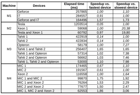
Table 2. Elapsed times and speedups for finding all the solutions for the 17-Queens.
To solve the 17-Queens Problem, the elapsed times ranged from about 20 minutes on Tesla to 58 seconds on Opteron.
When using all the devices on a machine and comparing the elapsed times against the fastest device on the same machine, the speedups ranged from 0.97 to 1.86, being slightly better than the ones achieved for Costas Array with 14 dots.
It was also possible to speed up the process of solving this CSP on M1, M3 and M4, but not on M2, although when adding Tesla, the elapsed times remained almost equal to when using only Xeon 1.
When using all the devices on a machine and comparing the elapsed times against the slowest device on the same machine, the speedups ranged from 1.73 to 19.8.
There are some factors that reduce the speedup that may be achieved when adding more devices, namely:
– Using more devices on a machine leads to a greater load of the host, because it will be responsible for setting up the additional devices and distributing the load between them. For example, when all devices of M4 were used, each MIC took about 6 seconds initializing before starting exploring search spaces, and that initialization is always done by the host (Xeon 2 on M4); – When using more devices, the search space is split into more sub-search
spaces to allow better load balancing, and the splitting process will take longer to complete.
6
Conclusion and future work
To our knowledge PHACT is the only existent constraint solver capable of using CPUs, GPUs and MICs (and other devices that are compatible with OpenCL) to speed up the solving process of CSPs. The results presented display speedups of up to about 2 when adding slower devices and up to about 35 when adding faster devices to solve the same CSPs. These results show that adding more devices to solve the same problem can speed up the process, even when the added devices are slower.
However, when the added device is much slower, it may affect the solver performance negatively and lead to a slight slowdown. This was noted when adding Tesla to work with Xeon 1 on M2.
Also, most computers and even some supercomputers include GPUs and PHACT allows using them to speed up the process of solving CSPs.
Although it is not fair to compare devices with such different architectures, on M1, Geforce was 1.1 times faster than I7 (8 threads) when using all cores of both devices. These results are much better than the ones achieved by Jenkins et al. in [5] which concluded that a GPU can only be 1.4 to 2.25 times as fast as a single CPU core, when exploring the backtracking paradigm.
Using the load-balancing techniques presented here allowed to achieve some good speedups, but better speedups can be achieved, because in the trials which results were presented here some devices finished their work before the remaining devices. This is mainly due to the fact that rank takes into account the time taken to be explore the last set of sub-search spaces, but some sub-search spaces take longer to explored than others leading to a difference between the time estimated for a device to finish his work and the actual time that it will take.
Currently, PHACT is being extended to solve optimization problems and to work also on Microsoft Windows. Afterwards, it will also be extended to run over distributed environments to use simultaneously multiple devices on interconnected machines.
Acknowledgments
Some of the experimentation was carried out on the khromeleque cluster of the University of ´Evora, which was partly funded by grants ALENT-07-0262-FEDER-001872 and ALENT-07-0262-FEDER-001876.
References
1. Arbelaez, A., Codognet, P.: A GPU implementation of parallel constraint-based local search. In: 22nd Euromicro International Conference on Parallel, Distributed and Network-Based Processing (PDP). pp. 648–655. PDP ’14, IEEE, Italy (2014) 2. Campeotto, F., Pal`u, A.D., Dovier, A., Fioretto, F., Pontelli, E.: Exploring the use of GPUs in constraint solving. In: Flatt, M., Guo, H.F. (eds.) PADL 2014. LNCS, vol. 8324, pp. 152–167. San Diego, CA, USA (January 2014)
3. Chu, G., Schulte, C., Stuckey, P.J.: Confidence-based work stealing in parallel constraint programming. In: Gent, I.P. (ed.) CP 2009. LNCS, vol. 5732, pp. 226– 241. Springer, Lisbon, Portugal (September 2009)
4. Du, P., Weber, R., Luszczek, P., Tomov, S., Peterson, G., Dongarra, J.: From CUDA to OpenCL: Towards a performance-portable solution for multi-platform GPU programming. Parallel Computing 38(8), 391–407 (August 2012)
5. Jenkins, J., Arkatkar, I., Owens, J., Choudhary, A., Samatova, N.: Lessons learned from exploring the backtracking paradigm on the GPU. In: Jeannot, E., Namyst, R., Roman, J. (eds.) Euro-Par 2011 Parallel Processing, Lecture Notes in Computer Science, vol. 6853, pp. 425–437. Springer (2011)
6. Mairy, J.B., Deville, Y., Lecoutre, C.: Integration of AI and OR Techniques in Constraint Programming: 11th International Conference, CPAIOR 2014, Cork, Ireland, pp. 235–250. Springer (2014)
7. Munshi, A., Gaster, B., Mattson, T.G., Fung, J., Ginsburg, D.: OpenCL Program-ming Guide. Addison-Wesley Professional, 1st edn. (2011)
8. Nickolls, J., Kirk, D. (eds.): Graphics and Computing GPUs, vol. 28. Morgan Kaufmann, 4 edn. (2009)
9. NVIDIA GeForce GTX 980 Featuring Maxwell, The Most Advanced GPU Ever Made. White paper, NVIDIA Corporation (2014)
10. Pedro, V.: Constraint Programming on Hierarchical Multiprocessor Systems. Ph.D. thesis, Universidade de ´Evora (2012)
11. Rolf, C.C., Kuchcinski, K.: Parallel solving in constraint programming. In: MCC 2010: Third Swedish Workshop on Multi-Core Computing (November 2010) 12. Roque, P., Pedro, V., Abreu, S.: Solving constraint satisfaction problems in GPUs.
In: Salgueiro, P., Nogueira, V. (eds.) JIUE 2015 - Actas das 5as Jornadas de In-form´atica da Universidade de ´Evora. Universidade de ´Evora (February 2015) 13. Roque, P., Pedro, V., Abreu, S.: Trials to Solve Constraint Satisfaction Problems in
GPUs (July 2015), Seminar 2 of PhD degree in Computer Science in Universidade de ´Evora (Portugal).
14. Roque, P., Pedro, V., Abreu, S.: Towards a multi-device constraints solver. In: Nogueira, V., Abreu, S. (eds.) JIUE 2016 - Actas das 6asJornadas de Inform´atica da Universidade de ´Evora. Universidade de ´Evora (March 2016)
15. R´egin, J.C., Rezgui, M., Malapert, A.: Embarrassingly parallel search. In: Schulte, C. (ed.) CP 2013, Uppsala, Sweden, September 16-20, 2013. Proceedings. Lecture Notes in Computer Science, vol. 8124, pp. 596–610. Springer (2013)
16. Schulte, C.: Parallel search made simple. In: Beldiceanu, N., Harvey, W., Henz, M., Laburthe, F., Monfroy, E., M¨uller, T., Perron, L., Schulte, C. (eds.) Proceedings of TRICS, a post-conference workshop of CP 2000. Singapore (September 2000) 17. Schulte, C., Duchier, D., Konvicka, F., Szokoli, G., Tack, G.: Generic constraint
development environment. http://www.gecode.org/
18. Werkhoven, B.V., Maassen, J., Seinstra, F., Bal, H.: Performance models for CPU-GPU data transfers. 2014 14th IEEE/ACM International Symposium on Cluster, Cloud and Grid Computing pp. 11–20 (2014)