SPATIAL PATTERNS AND RELATIONS WITH SITE
FACTORS IN A CAMPOS GRASSLAND
UNDER GRAZING
FOCHT, T. and PILLAR, V. D.Departamento de Ecologia, Universidade Federal do Rio Grande do Sul, CEP 91540-000, Porto Alegre, RS, Brazil Correspondence to: Valério DePatta Pillar, Departamento de Ecologia, Universidade Federal do Rio Grande do Sul, Avenida Bento Gonçalves, 9500, CEP 91540-000, Porto Alegre, RS, Brazil, e-mail: [email protected]
Received January 14, 2002 – Accepted April 12, 2002 – Distributed August 31, 2003 (With 2 figures)
ABSTRACT
Spatial distribution patterns and their relations with environmental factors at different scales were identified in ca. 100-ha grassland under cattle and sheep grazing, in Eldorado do Sul, RS, Brazil (30o05’S, 51o40’W). The field survey used 138 0.5
x 0.5 m quadrats located systematically on transects
along relief gradients. The quadrats were arranged in groups of 3 contiguous quadrats, which were pooled for the analysis, thus forming 46 quadrats 1.5 x 0.5 m, in this way defining two observation
scales. Vegetation description involved recording the presence and the visual estimation of cover-abundance of species in each quadrat. A total of 148 species belonging to 30 families was detected. The environmental conditions at each site were described by 30 variables related to soil chemical and physical properties, slope, exposure and relief position. Data analysis used cluster analysis, evalua-tion of group partievalua-tion sharpness, ordinaevalua-tion, significance of ordinaevalua-tion axes, evaluaevalua-tion of environmental congruence and randomization testing. The results of the analysis with 46 quadrats supported those found with 138 quadrats. The vegetation patterns in the study area are associated to relief position and other related factors such as soil moisture. Two clearly defined grassland community types were detected, one occurring on the slopes and another on the wet lowlands.
Key words: grassland vegetation, spatial distribution patterns, environmental factors, scale, statisti-cal analysis.
RESUMO
Padrões espaciais e suas relações com fatores de ambiente de um campo pastejado
Padrões de distribuição espacial e suas relações com fatores ambientais, em diferentes escalas, são identificados em uma área de vegetação campestre de aproximadamente 100 ha sob pastejo ovino e bovino em Eldorado do Sul, RS, Brasil (30o05’S, 51o40’W). O levantamento no campo foi efetuado em 138 unidades amostrais de 0,5 x 0,5 m localizadas sistematicamente ao longo de gradientes de
relevo. As unidades amostrais foram dispostas em conjuntos de 3 quadros contíguos, que foram agru-pados para análise, formando 46 quadros de 1,5 x 0,5 m, definindo, desta forma, duas escalas de
da vegetação na área de estudo estão relacionados à posição no relevo e a outros fatores associados, tais como umidade do solo. Dois grupos nítidos de comunidades campestres foram detectados, um ocor-rendo nas encostas e outro ocorocor-rendo nas baixadas úmidas.
Palavras-chave: vegetação campestre, padrões de distribuição espacial, fatores ambientais, escala, análise estatística.
INTRODUCTION
Natural grassland vegetation known as “Cam-pos” presently covers almost half of the territory of the state of Rio Grande do Sul in Brazil. Between 1970 and 1996 about one-third of the area formerly covered by natural grassland was transformed into other land uses, mainly for crop cultivation (IBGE, 1996). On the one hand this drastic land use changed points to a failure in the Brazilian legislation in protecting native grassland at the same level as forest areas are now protected. On the other hand, with such territory extent and increasing natural habitat destruction, the search for knowledge about vegetation structure and composition in the “Cam-pos” could help to find ways for their protection and sustainable use.
The study of plant communities is essentially comparative. The physiognomy of a vegetation stand is the result of its composition in terms of plant species or types. Spatial and temporal variation in the arrangement of plant community components may be perceived by means of a classification of the communities into types. The accepted operational definition of a plant community is a unit with arbi-trary limits set by the researcher and containing plant organisms (Palmer & White, 1994). The same authors also point out that the existence of integration or interaction among the components should not be a condition to call such unit as community. Instead, whether and at which degree the components interact may be part of the study objectives. Other authors also gave important contributions to this conceptual discussion (Keddy, 1993; Wilson & Chiarucci, 2000). Furthermore, the distribution of plants in space and time is related to or dependent on other biotic and abiotic factors (Pillar et al., 1992; Pillar & Boldrini, 1996).
The convolution of biotic and abiotic inte-ractions gives rise to non-random arrangements of plant organisms forming a heterogeneous and com-plex structure (Orlóci, 1993). Indeed, it is a fact that
to be found repeatedly in a given study area, revea-ling patterns which can be related to site factors (Kershaw, 1973; Moloney, 1993; Orlóci, 1993; Boldrini & Eggers, 1997; Crawley, 1997). It is likely that only one factor cannot be accepted as the cause of a given plant distribution, for there are many other interacting factors (Whittaker, 1967). Gould (1991), criticizing the use of factorial analysis in IQ tests, warned against the temptation of reifying an abs-traction, that is, thinking that there is something real underlying a complex of highly correlated variables. This temptation should be avoided since it may not correspond to a truth in nature. Yet, it is possible, based on survey data, to search for critical factors related to community patterns. Whether they cause or not the patterns will define hypothesis that should be further evaluated, in a process of successive approximation (Orlóci, 1993).
In the study of vegetation patterns, therefore, the sampling units (the communities in our sense) are cross sections of a continuum and are set by the investigator, which makes the sampling more compli-cated than when dealing with individuals. Furthermore, due to non-random arrangements, the scale (size of the sampling unit) matters, affecting the perception of patterns (Pillar, 2001). The decisions in defining the design to sample plant communities refer to the sampling unit size, number and method of location. These should be dependent on the context and objec-tives (Kenkel et al., 1989), therefore the conclusions are affected by the sampling design (Juhász-Nagy & Podani, 1983; Goedickemeier et al., 1997).
commu-interpreted in terms of other variables. Moreover, most of the relations and connections are expressed in a non-linear way (Capra, 1997; Franceschi & Prado, 1989; Orlóci, 1993; Pielou, 1984; Podani, 1994; van der Maarel, 1980). In addition, since the scale matters, the study of plant communities should contemplate different sampling unit sizes (Greig-Smith, 1952; Levin, 1992; Podani et al., 1993). The sizes may vary from the smaller sizes covering a vegetation patch to larger ones involving landscape units. The use of contiguous sampling units allows the definition a posteriori of larger units in the data analysis.
The description of plant communities delimited by permanent quadrats located on environmental gradients, more specifically relief gradients, is one of the ways to study the processes and factors involved in the spatial distribution of plants and plant communities, which defines the vegetation’s phy-siognomy.
In this paper the aim is to identify plant commu-nity patterns and relate them to environmental variables in natural grassland (Campos) located in the research station of the Federal University of Rio Grande do Sul (EEA/UFRGS) in Eldorado do Sul, RS, Brazil. We take into account two scales of observation and evaluate hypothesis about relevant environmental factors related to the community patterns.
STUDY AREA
The survey was carried out in approximately 100 ha of grazed “Campos” (natural grassland) in the EEA/UFRGS, located at 30°05’S, 51°40’W, in Eldorado do Sul, RS, Brazil. The altitude in the study area is between 20 and 70 m. The climate is humid subtropical, classified as Cfa in Köppen’s clas-sification, which is the predominant type in the lower altitudes in the south of Brazil (Moreno, 1961; Trewartha & Horn, 1980). Extensive alluvial plains and smoothly undulated hills characterize the relief, with more or less humid depressions and valleys (Pillar & Boldrini, 1996; Boldrini, 1997). The soils on the hills are mostly red dystrophic argisols and planosols on the lowlands (Mello et al., 1966; Embrapa, 1999).
A preliminary assessment of the physiognomy and floristic composition indicated that the vegetation is a mixture of short and tall grasses, interstitial short
herbs and short to tall shrubs. The area was under cattle and sheep grazing, with patches intensively grazed mostly covered by Paspalum spp. and Axonopus affinis interspersed by ungrazed patches mostly covered by unpalatable plants of Eryngium horridum, Baccharis trimera and tall grasses such as Aristida jubata and Andropogon lateralis. The grazed patches on convex slopes show more bare soil than on the concave slopes. At the upper convex slopes the soil is dryer and the vegetation is mainly composed of Paspalum notatum, Aristida jubata, Aristida laevis, Piptochaetium montevidense, Eryngium ciliatum and Eryngium horridum. On the moist lower concave slopes the presence of Andropogon lateralis and Baccharis trimera is more common. On the wet lowland extreme environment the most frequently species are Eleocharis maculosa, Panicum sabulorum, Paspalum pumilum and Centella asiatica. Therefore, we conjectured the existence of three community types is conjectured, which are mostly related to relief position. More details on the study area can be found in Focht (2001).
METHODS
For the sampling we used 18 transects, located preferentially on relief gradients from the top of the hills in direction of the lowlands, taking into account different slopes and exposures. Guided by the transects 138 permanent quadrats of 0.5 x 0.5 m
(henceforth denominated small quadrats) were marked, grouped in sets of three contiguous quadrats, thus forming 46 quadrats of 0.5 x 1.5 m (henceforth
denominated large quadrats). In this way two study scales could be considered. The quadrats were located on three positions of the transects (upper, mid slope and lower) aiming at visually perceived homogeneous sites. The quadrats on the lower positions were not necessarily on the lowland wet sites.
The plant community composition in each 0.5 x
When the species identity of an individual plant could not be determined either due to the lack of reproductive parts or knowledge about the taxonomic group, it was identified at the genus level.
The soil around each large quadrat of 1.5 x
0.5 m was sampled in May 2000. The soil was analyzed by standard methods (Tedesco et al., 1995) for the following descriptors: % of clay, % of organic matter, pH and exchangeable contents of P, K, Al, Ca, Mg, S, Zn, Cu, B and Mn, cation exchange capacity (CEC) and derived indexes of saturation of CEC with aluminum and hydrogen, saturation of CEC with bases, saturation of CEC with Al, Ca/Mg ratio, Ca/K ratio and Mg/K ratio. Soil moisture regime at the quadrat’s site was evaluated by visual and tactile observation using the following scale: 1: moist only after a rain, 2: dry only in short drought periods, and 3: always moist. Bare soil and cover by litter material on the soil were visually estimated in each small quadrat using the Braun-Blanquet scale already mentioned. The relief position of the quadrat was recorded using a semi-quantitative scale: 1 (top and convex slope), 2 (concave slope), and 3 (lowland). The average vegetative stand height and the average thickness of the litter layer on the soil were also estimated for each small quadrat. Potential solar radiation on the quadrat was estimated for each season on the basis of its slope and exposure and radiation data from the meteorological station at EEA/UFRGS in the year 1999, according to the methodology described in Forseth & Norman (1983).
The data on community composition were initially arranged in a matrix of species by commu-nities (small quadrats). The cover-abundance sym-bols of the Braun-Blanquet scale (r, +, 1, 2, 3, 4 and 5) were replaced by values according to van der Maarel (1979): 1, 2, 3, 5, 7, 8, and 9, respectively. The data analysis was performed separately at the two scales of quadrat size (small and large). The community composition data matrix for the large quadrats was analytically found by computing the average cover-abundance value for each species based on the three small contiguous quadrats nested in the large quadrat. The same procedure was used to find average values for environmental variables in the large quadrats when the variable was evaluated only in the small quadrats.
to statistically test for the association between community composition (in the large quadrats) and environmental conditions.
RESULTS AND DISCUSSION
The survey carried out in the 138 small qua-drats allowed to find 148 species belonging to 30 families (Table 1). By cluster analysis two groups of quadrats were identified with this data set. The groups were considered as two distinct community types, as indicated by the test for group sharpness (Pillar, 1999b). Also two distinct community types were identified by cluster analysis with the data from the large quadrats. The communities (quadrats) belonging to the same group tend to be more similar than communities belonging to different groups. At this clustering level there was no evident effect of the observation scale, since the small quadrats into the large ones by nesting showed the classification produced was nearly the same. Henceforth we will give emphasis to the results with the large quadrats. More than two community groups could be defined on the basis of the cluster analyses but the groups would not be sharp enough in the sense that they would not be sufficiently stable to reappear if the same sampling universe were resampled (Pillar, 1999b). Details on the results of the cluster analyses can be found in Focht (2001).
Table 2 shows the average values for the environmental variables in each group formed with the large quadrats on the basis of floristic data. The inspection of the table indicates which variables are more associated to the community types: relief position and associated variables such as soil mois-ture, clay, K and Ca content.
The conjectured existence of three distinct community types was not confirmed by data analysis, since only two sharp groups were defined. Two community types are clearly separated in two relief positions: Quadrats belonging to group 1 are located on the upper convex slopes and lower concave slopes, while quadrats belonging to group 2 are on the wet lowland. The species found in the survey were grouped according to the percentage of pre-sence in each community type. In this way it could be identified which species are characteristic of each community type and which are more generalist ones (Table 1). In Table 1 the first species group contains
the species that occur in more than 50% of the quadrats in both community types, which means that they are the species with the greatest ecological plasticity, considering that they occur in a wide environmental range. The second species group contains the species present in more than 50% of the quadrats belonging to community type 1 and thus is characteristic of dryer sites. The species in the third group occur in more than 50% of the quadrats in community type 2 and are indicators of wet lowland conditions. The fourth species group does not have clear preferences since the species are present in less than 50% of the quadrats in any of the community types.
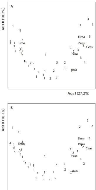
The ordination results reveal the spatial distri-bution pattern of the communities. In Fig. 1 the quadrats are arranged solely according to the main ordination axes generated from the species com-position. The horseshoe-like arrangement of the communities in the ordination scatter diagram is an indication of non-linear responses of species, not an artifact that would require some kind of detrending (Podani, 1994). It could be seen that this arrangement matches very well with the soil moisture gradient (Fig. 1A), and soil moisture is mostly a consequence of relief position. Based on the species mostly correlated with the ordination axes the gradient could be interpreted in terms of species composition. E. horridum is typical of communities on dryer sites (soil moisture class 1) located on convex slopes (upper left corner of the diagram). As we move from left to right on the diagram along the moisture gradient there is a gradual substitution of species. Andropogon lateralis is typical of communities on moist sites (soil moisture class 2) on lower concave slopes. Panicum sabulorum, Paspalum pumilum, Centella asiatica and Eleocharis maculosa are typical of the wet lowland areas (soil moisture class 3).
Presence (%) in community types
Average cover-abundance when present Species 1 2 1 + 2 1 2 1 + 2
Species with presence > 50% in both community types
Paspalum notatum 97.0 61.5 87.0 4.1 3.5 4.0
Andropogon lateralis 75.8 100 82.6 4.0 4.2 4.0
Baccharis trimera 72.7 76.9 73.9 1.9 0.9 1.6
Rhynchospora microcarpa 51.5 92.3 63.0 1.6 2.5 2.0
Species with presence > 50% only in community type 1
Oxalis corniculata 97.0 30.8 78.3 2.0 0.7 1.1
Piptochaetium montevidense 93.9 38.5 78.3 2.6 1.3 1.1
Eryngium horridum 78.8 7.7 58.7 3.8 1.7 3.7
Dichondra sericea 75.8 15.4 58.7 1.6 0.7 1.5
Desmodium incanum 72.7 23.1 58.7 1.4 1.6 1.4
Ruellia morongii 66.7 30.8 56.5 1.2 1.1 1.2
Evolvolus sericeus 66.7 0 47.8 1.2 0 1.2
Paspalum paucifolium 63.6 7.7 47.8 1.6 0.7 1.6
Chevreulia sarmentosa 60.6 23.1 50.0 1.1 0.9 1.1
Stylosanthes leiocarpa 57.6 46.2 54.3 1.2 1.1 1.3
Aristida jubata 54.5 7.7 41.3 2.9 1.7 2.8
Aristida laevis 51.5 15.4 41.3 2.2 1.3 2.1
Species with presence > 50% only in community type 2
Paspalum pumilum 6.1 100 32.6 1.0 3.4 3.1
Centella asiatica 18.2 92.3 39.1 1.7 3.2 2.7
Diodia sp. 24.2 84.6 28.3 0.9 3.9 1.0
Eleocharis maculosa 3.0 84.6 26.1 2.7 3.9 3.8
Panicum sabulorum 24.2 76.9 39.1 1.3 1.3 1.3
Tibouchina gracilis 12.1 69.2 28.3 1.3 1.1 1.2
Desmodium adscendens 30.3 69.2 41.3 1.4 1.0 1.2
Axonopus affinis 27.3 61.5 37.0 2.1 1.7 1.9
Other species
Vernonia nudiflora 42.4 38.5 41.3 1.6 1.0 1.4
Hypoxis decumbens 42.4 38.5 41.3 1.1 0.7 1.1
Andropogon selloanus 45.5 30.8 39.1 1.7 1.1 1.6
Chevreulia acuminata 42.4 30.8 37.0 0.9 0.7 0.9
Oxaliscorymbosa 45.5 23.1 37.0 0.8 3.4 0.7
Richardia sp. 48.5 0 34.8 1.4 0 1.4
TABLE 1
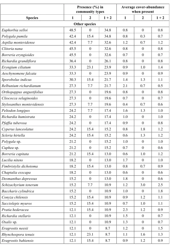
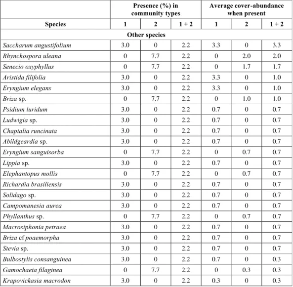
List of species found in the survey of 46 1.5 x 0.5 m quadrats on natural grassland in Eldorado do Sul, RS, Brazil. Percentage of presence and average cover-abundance values
TABLE 1 (continued.)
Presence (%) in community types
Average cover-abundance when present Species 1 2 1 + 2 1 2 1 + 2
Other species
Euphorbia selloi 48.5 0 34.8 0.8 0 0.8
Polygala pumila 42.4 15.4 34.8 0.8 0.3 0.7
Aspilia montevidense 42.4 7.7 32.6 1.2 0.7 1.2
Clitoria nana 45.5 0 32.6 0.8 0 0.8
Borreria eryngioides 45.5 0 32.6 0.7 0 0.7
Richardia grandiflora 36.4 0 26.1 0.8 0 0.8
Eryngium ciliatum 33.3 23.1 23.9 0.9 1.0 1.4
Aeschynomene falcata 33.3 0 23.9 0.9 0 0.9
Sporobolus indicus 30.3 15.4 21.7 1.4 1.3 1.1
Relbunium richardianum 27.3 7.7 21.7 2.1 0.7 0.5
Orthopappus angustifolius 27.3 0 19.6 0.8 0 0.8
Cliococca selaginoides 27.3 0 19.6 0.7 0 0.7
Stylosanthes montevidensis 27.3 7.7 19.6 0.4 0.7 0.6
Peltodon longipes 24.2 7.7 17.4 1.6 1.3 1.0
Richardia humistrata 24.2 0 17.4 1.0 0 1.0
Pfaffia tuberosa 24.2 0 17.4 0.9 0 0.8
Cyperus lanceolatus 24.2 15.4 15.2 0.8 1.8 1.2
Scleria hirtella 24.2 15.4 15.2 0.6 1.3 1.2
Polygala sp. 21.2 0 15.2 1.0 0 1.0
Cuphea sp. 21.2 0 15.2 0.7 0 0.6
Borreria capitata 21.2 15.4 13.0 0.6 1.0 1.2
Lucilia nitens 18.2 0 13.0 1.7 0 1.0
Fimbristylis dichotoma 18.2 15.4 13.0 0.8 0.7 0.9
Chaptalia exscapa 18.2 0 13.0 0.6 0 0.6
Desmanthus depressus 15.2 0 13.0 1.8 0 0.6
Schizachyrium tenerum 15.2 7.7 10.9 1.2 3.0 2.5
Baccharis cylindrica 15.2 0 10.9 1.0 0 1.8
Conyza chilensis 15.2 15.4 10.9 0.9 1.2 1.1
Sacciolepis myuros 15.2 15.4 10.9 0.7 1.0 1.1
Pratia hederacea 12.1 15.4 10.9 2.3 1.2 0.9
Richardia stellaris 12.1 0 10.9 1.5 0 0.7
Oxalis sp. 12.1 0 10.9 1.3 0 0.7
Eragrostis neesii 12.1 0 8.7 1.2 0 1.5
Rhynchospora tenuis 12.1 23.1 8.7 1.1 1.6 1.3
TABLE 1 (continued.)
Presence (%) in community types
Average cover-abundance when present Species 1 2 1 + 2 1 2 1 + 2
Other species
Cuphea glutinosa 12.1 0 8.7 0.8 0 0.9
Panicum decipiens 12.1 0 8.7 0.7 0 0.8
Fimbristylis diphylla 12.1 15.4 8.7 0.7 1.0 0.8
Ruellia sp. 12.1 7.7 8.7 0.7 0.3 0.8
Sida rhombifolia 12.1 0 8.7 0.7 0 0.7
Justicia sp. 12.1 0 8.7 0.6 0 0.7
Waltheria douradinha 12.1 0 8.7 0.3 0 0.7
Zornia sp. 12.1 0 8.7 0.3 0 0.3
Paspalum sp. 9.1 23.1 6.5 1.6 1.9 1.9
Galianthe fastigiata 9.1 0 6.5 1.1 0 1.6
Bulbostylis juncoides 9.1 7.7 6.5 1.1 0.7 1.3
Cyperus tener 9.1 7.7 6.5 0.9 1.7 1.2
Glandularia sp. 9.1 0 6.5 0.9 0 1.1
Schizachyrium microstachyum 9.1 15.4 6.5 0.8 0.7 1.0
Sida sp. 9.1 7.7 6.5 0.7 0.7 0.9
Paspalum plicatulum 9.1 0 6.5 0.7 0 0.8
Setaria geniculata 9.1 0 6.5 0.7 0 0.7
Pterocaulon sp. 9.1 0 6.5 0.6 0 0.7
Pterocaulon rugosum 9.1 0 6.5 0.4 0 0.6
Sisyrinchium sp. 6.1 7.7 6.5 1.7 0.7 0.6
Verbena lindmanii 6.1 0 6.5 1.3 0 0.4
Tibouchina asperior 0 15.4 4.3 0 2.0 2.0
Drymaria cordata 6.1 0 4.3 1.3 0 1.3
Paspalum nicorae 6.1 0 4.3 1.3 0 1.0
Crotalaria tweediana 6.1 0 4.3 1.0 0 1.0
Mecardonia sp. 6.1 0 4.3 1.0 0 0.8
Borreria verticillata 6.1 0 4.3 1.0 0 0.8
Andropogon macrothrix 6.1 7.7 4.3 1.0 0.7 0.8
Commelina sp. 6.1 0 4.3 1.0 0 0.8
Vernonia flexuosa 6.1 0 4.3 0.8 0 0.7
Brachiaria plantaginea 6.1 0 4.3 0.8 0 0.7
Baccharis sp. 6.1 0 4.3 0.7 0 0.7
Senecio selloi 6.1 0 4.3 0.7 0 0.7
Fimbristylis cf autumnalis 0 15.4 4.3 0 0.5 0.5
Xyris jupicai 6.1 7.7 4.3 0.3 0.3 0.3
TABLE 1 (continued.)
Presence (%) in community types
Average cover-abundance when present Species 1 2 1 + 2 1 2 1 + 2
Other species
Saccharum angustifolium 3.0 0 2.2 3.3 0 3.3
Rhynchospora uleana 0 7.7 2.2 0 2.0 2.0
Senecio oxyphyllus 0 7.7 2.2 0 1.7 1.7
Aristida filifolia 3.0 0 2.2 3.3 0 1.0
Eryngium elegans 3.0 0 2.2 3.3 0 1.0
Briza sp. 0 7.7 2.2 0 1.0 1.0
Psidium luridum 3.0 0 2.2 0.7 0 0.7
Ludwigia sp. 3.0 0 2.2 0.7 0 0.7
Chaptalia runcinata 3.0 0 2.2 0.7 0 0.7
Abildgeardia sp. 3.0 0 2.2 0.7 0 0.7
Eryngium sanguisorba 0 7.7 2.2 0 0.7 0.7
Lippia sp. 3.0 0 2.2 0.7 0 0.7
Elephantopus mollis 0 7.7 2.2 0 0.7 0.7
Richardia brasiliensis 3.0 0 2.2 0.7 0 0.7
Solidago sp. 3.0 0 2.2 0.7 0 0.7
Campomanesia aurea 3.0 0 2.2 0.7 0 0.7
Phyllanthus sp. 0 7.7 2.2 0 0.7 0.7
Macrosiphonia petraea 3.0 0 2.2 0.7 0 0.7
Briza cf poaemorpha 3.0 0 2.2 0.7 0 0.7
Stevia sp. 3.0 0 2.2 0.7 0 0.7
Bulbostylis consanguinea 3.0 0 2.2 0.7 0 0.3
Gamochaeta filaginea 0 7.7 2.2 0 0.3 0.3
Krapovickasia macrodon 3.0 0 2.2 0.3 0 0.3
The test evaluating the significance of the ordination axes indicated that only axis 1 was significant in both ordinations with large and small quadrats. Axis 2 and the other axes were not signi-ficant, that is, the ordination on these axes was not distinguishable from an ordination obtained if the variables were completely uncorrelated (Pillar, 1999a).
The species richness in community type 1 is higher than in community type 2, which becomes evident by inspection of Table 1. The possible cause of this fact is that the environmental conditions on the slopes may present greater seasonal fluctuation
Variable Labels Unit Group 1 Group 2
Stand height ave cm 11.98 10.50
Litter cover com 1–9 class 6.02 5.00
Litter thickness alm cm 0.98 0.73
Bare soil sod 1–9 class 2.44 1.38
Relief position of the quadrat poq 1–3 class 1.76 3.00
Soil moisture regime ums 1–3 class 1.21 2.77
Clay arg % 20.97 13.85
pH ph – 4.83 4.57
P p mg.L–1 3.13 3.13
K k mg.L–1 170.33 103.08
Organic matter mo % 3.76 4.62
Al+++ alt cmol.c.L–1 0.46 1.04
Ca cat cmol.c.L–1 2.05 1.43
Mg mgt cmol c.L–1 1.38 0.75
Al+++ plus H+ alh cmol.c.L–1 6.05 7.56
Cation exchange capacity (CEC) cec cmol.c.L–1 9.68 10.07
Saturation of CEC with bases ctb % 37.56 26.77
Saturation of CEC with Al cta % 5.00 9.33
Ca/Mg ratio cam – 1.66 2.02
Ca/K ratio cal – 4.91 5.48
Mg/K ratio mgk – 3.15 2.87
S s mg.L–1 9.57 10.64
Zn zn mg.L–1 2.91 2.71
Cu cu mg.L–1 1.27 1.49
B b mg.L–1 0.67 0.60
Mn mn mg.L–1 40.00 33.54
Summer potential radiation rve (MJ.m–2.day) 27.38 27.43
Autumn potential radiation rou (MJ.m–2.day) 17.27 17.29
Winter potential radiation rin (MJ.m–2.day) 9.562 9.569
Spring potential radiation rpr (MJ.m–2.day) 20.93 21.10
TABLE 2
Fig. 1 –Ordination of 46 grassland communities (quadrats 1.5 x 0.5 m) in Eldorado do Sul, RS, Brazil. The scatter diagram is defined by ordination axes 1 and 2 generated by principal coordinates analysis from chord distances using the species composition data. The percentage of total variation represented by the axes is indicated. The species plotted on the diagram had a correlation |r| > 0.6 with at least one of the axes: Erho = E. horridum; Anla = A.lateralis; Pasa = P. sabulorum; Ceas = C. asiatica; Papu = P. pumilum;
Fig. 2 – Profile of maximum congruence between vegetation variation on the first ordination axis (Fig. 1) and environmental variation given by the variables indicated on the abscissa cumulatively from left to right. Legends of the variables should be read vertically and are indicated in Table 2.
The evaluation of congruence between variation in vegetation composition on the first ordination axis, since only this axis was significant, and environmental conditions indicated that soil moisture was the variable that when used alone produced maximum correlation (Fig. 2). When other variables were included the correlation became lower, however for sets with two variables it was maximum when soil moisture was combined with relief position.
Comparing both observation scales (large and small quadrats), no remarkable differences were found in the results. The analysis with the 46 large quadrats reflected the same variation found in the 138 small quadrats. This may indicate that the three small contiguous quadrats are mainly not inde-pendent, since they are very close in space, some-times with the same individual being observed across neighboring quadrats.
The results show that the main factors related to vegetation variation in the studied grassland are linked to relief position. Actually, variables such as soil moisture regime, soil cationic exchange capacity, pH and exchangeable Al and the soil type are clearly a consequence of relief position. These findings are supported by studies on similar grassland in the EEA/UFRGS (Pillar et al., 1992; Boldrini,
1993) and other vegetation elsewhere (Wierenga et al., 1987; Franceschi & Prado, 1989). Grazing may be also an important factor but it was not evaluated in this study. According to Whittaker (1967), only one factor cannot be accepted as the cause of plant distribution, since there is a group of variables interacting. The network of relations linking the biotic components and abiotic factors is probably so complicate and huge that they are mathematically intractable (Gould, 1991; Orlóci, 1993). Therefore, the results of a survey will always be a simplification, but may be the best information available.
Using multivariate analysis of variance it was tested whether quadrat groups defined by selected environmental variables (factors) were significantly different with regard to the complete species composition (Pillar & Orlóci, 1996). The analysis was done for each environmental variable. It was found that quadrat groups defined by soil moisture classes were significantly different (p < 0.05). The same was found for groups defined by relief position, soil cationic exchange capacity, litter cover, soil pH and soil exchangeable Al. These variables were significantly related to the species composition of the communities. No significant differences in species composition were found for factors such as soil P, stand height and winter potential radiation (p > 0.05).
CONCLUSIONS
The vegetation patterns in the study area are associated to relief position and other related factors such as soil moisture.
Two clearly defined grassland community types were detected, one occurring on slopes and another on wet lowlands.
Both scales of observation (small and large quadrats) revealed nearly the same patterns.
Acknowledgments — This work was supported by a scholarship
from CAPES received by T.F. and by a grant and fellowship received by V.P. from CNPq (Brazil). We thank Juliana Cunha for helping with the translation of the manuscript to English.
REFERENCES
BOLDRINI, I. I., 1993, Dinâmica de vegetação de uma pastagem natural sob diferentes níveis de oferta de forragem e tipos de solos, Depressão Central, RS. Tese de Doutorado,
Faculdade de Agronomia, UFRGS, Porto Alegre, 262p. BOLDRINI, I. I., 1997, Campos do Rio Grande do Sul:
caracterização fisionômica e problemática ocupacional. Bol. Inst. Biocienc./UFRGS, 56: 1-39.
BOLDRINI, I. I. & EGGERS, L., 1997, Directionally of sucession after grazing exclusion in grassland in the South of Brazil.
Coenoses, 12: 63-66.
BRAUN-BLANQUET, J., 1964, Fitossociología: bases para el estudio de las comunidades vegetales (Pflanzensoziologie. Grundzüge der Vegetationskunde).Trad. 3. ed. rev. aum. Blume, Madrid, 819p.
CAPRA, F., 1997, A teia da vida. Cultrix, São Paulo, 256p.
CRAWLEY, M. J., 1997, The structure of plant communities.
In: Plant ecology. 2. ed., Blackwell, Oxford.
DIGBY, P. G. N. & KEMPTON, R. A., 1987, Multivariate analysis of ecological communities. Chapman & Hall,
London, 206p.
EMBRAPA, 1999, Classificação dos solos brasileiros.
EMBRAPA, Brasília, 412p.
FEOLI, E. & ORLÓCI, L., 1985, Species dispersion profiles of anthropogenic grasslands in the Italian Eastern Pre-Alps.
Vegetatio, 60: 113-118.
FOCHT, T., 2001, Padrões espaciais em comunidades vegetais de um campo pastejado e suas relações com fatores de ambiente. Dissertação de Mestrado, Departamento de Ecologia, UFRGS, Porto Alegre, 167p.
FORSETH, I. N. & NORMAN, J. M., 1983, Modelling of solar irradiance, leaf energy budget and canopy photosynthesis and production in a changing environment. A field and laboratory manual. Chapman & Hall, London. FRANCESCHI, E. A. & PRADO, D. E., 1989, Distribution of
herbaceous communities of the River Parana Valley along an elevation gradient after a catastrophic flood. Coenoses,
4: 47-53.
GOEDICKEMEIER, I., WILDI, O. & KIENAST, F., 1997, Sampling for vegetation survey: some properties of a GIS-based stratification compared to other statistical sampling methods. Coenoses, 12: 43-50.
GOULD, S. J., 1991, A falsa medida do homem. Martins Fontes,
São Paulo, 369p.
GREIG-SMITH, P., 1952, The use of random and contiguous quadrats in the study of the structure of plant communities.
Ann. Bot., 62: 293-316.
IBGE, 1996, Censo Agropecuário de 1995-1996: Rio Grande do Sul. Disponível em: HYPERLINK <http://www.ibge.gov.br/
ibge/estatistica/agropecuaria/censoagro/43/utiliza.shtm>< http://www.ibge.gov.br/ibge/estatistica/agropecuaria/ censoagro/43/utiliza.shtm>. Acesso em: 20 jan. 2001. JUHÁSZ-NAGY, P. & PODANI, J., 1983, Information theory
methods for the study of spatial processes and sucession.
Vegetatio, 51: 129-140.
KEDDY, P., 1993, Do ecological communities exist? A reply to bastow Wilson. J. Veg. Sci., 4: 135-136.
KENKEL, N. C., JUHÁSZ-NAGY, P. & PODANI, J., 1989, On sampling procedures in populations and community ecology.
Vegetatio, 83: 195-207.
KERSHAW, K. A., 1973, Quantitative and dynamic plant ecology. 2. ed., Edward Arnold, London, 308p. LEVIN, A. S., 1992, The problem of pattern and scale in ecology.
Ecology, 73: 1943-1967.
MELLO, O. de, LEMOS, R. C. de, ABRÃO, P. U., AZOLIN, M. A. D., SANTOS, M. da C. L. dos & CARVALHO, A. P., 1966, Levantamento em série dos solos do Centro Agronômico.
Revista da Faculdade de Agronomia e Veterinária da Universidade Federal do Rio Grande do Sul, 8: 7-155.
MOLONEY, K. A., 1993, Determining process through pattern: reality or fantasy? In: S. A. Levin, T. M. Powell & J. H. Steele, Patch dynamics lecture notes in biomathematics.
MORENO, J. A., 1961, Clima do Rio Grande do Sul. Secretaria da Agricultura, Porto Alegre, 41p.
MUELLER-DOMBOIS, D. & ELLENBERG, H., 1974, Aims and methods of vegetation ecology. J. Wiley, New York, 547p.
ORLÓCI, L., 1978, Multivariate analysis in vegetation research.
2. ed., W. Junk Publishers, The Hague, 451p.
ORLÓCI, L., 1993, The complexities and scenarios of ecosystem analysis. In: G. P. Patil & C. R. Rao (eds.), Multivariate environmental statistics. Elsevier, Amsterdam, pp. 423-432.
PALMER, M. W. & WHITE, P. S., 1994, On the existence of ecological communities. Journal of Vegetation Science,5: 279-282.
PIELOU, E. C., 1984, The interpretation of ecological data – a primer on classification and ordination. John Wiley & Sons, New York, 263p.
PILLAR, V. D., 1997, Multivariate exploratory analysis and randomization testing with MULTIV. Coenoses, 12: 145-148.
PILLAR, V. D., 1999a, The bootstrapped ordination re-examined.
J. Veg. Sci., 10: 895-902.
PILLAR, V. D., 1999b, How sharp are classifications? Ecology,
80: 2508-2516.
PILLAR, V. D., 2000a, SYNCSA: software integrado para análise multivariada de comunidades baseada em caracteres, dados de ambiente, avaliação e testes de hipóteses. Departamento de Ecologia, Universidade Federal do Rio Grande do Sul, Porto Alegre (versão para Macintosh).
PILLAR, V. D., 2000b, MULTIV: aplicativo para análise multivariada e testes de hipóteses. Departamento de Ecologia, Universidade Federal do Rio Grande do Sul, Porto Alegre.
PILLAR, V. D., 2001. Suficiência amostral. In: Bicudo, C. & Bicudo, D. Amostragem em limnologia. Ed. Universidade de Maringá (in press).
PILLAR, V. D. & BOLDRINI, I. I., 1996, Lindman e a ecologia da vegetação campestre do Rio Grande do Sul. Ciência e Ambiente, 13: 87-97.
PILLAR, V. D., JACQUES, A. V. A. & BOLDRINI, I., 1992, Fatores de ambiente relacionados à variação da vegetação de um campo natural. Pesq. Agropec. Bras., 27: 1089-1101. PILLAR, V. D. & ORLÓCI, L., 1993, Character-based community analysis: the theory and an application program. SPB Academic Publishing, The Hague (Ecological Compu-tations Series; vol. 5).
PILLAR, V. D. & ORLÓCI, L., 1996, On randomization testing in vegetation science: multifactor comparison of relevé groups. J. Veg. Sci., 7: 585-592.
PODANI, J., 1994, Multivariate data analysis in ecology and systematics. SPB Academic Publishing, The Hague, 316p. PODANI, J., CZÁRÁN, T. & BARTHA, S., 1993, Pattern, area and diversity: the importance of spatial scale in species assemblages. Abstracta Botanica, 17: 37-51.
TEDESCO, M. J., GIANELLO, C., BISSANI, C. A., BOHNEN, H. & VOLKWEISS, S. J., 1995, Análise de solos, plantas e outros materiais. 2. ed., Faculdade de Agronomia, UFRGS, Porto Alegre, 174p.
TREWARTHA, G. T. & HORN, L. H., 1980, Köppen’s classification of climates. In: An Introduction to climate.
McGraw-Hill, New York, pp. 397-403.
VAN DER MAAREL, E., 1979, Transformation of cover-abundance values in phytosociology and its effects on community similarity. Vegetatio, 39: 97-114.
VAN DER MAAREL, E., 1980, On the interpretability of ordination diagrams. In: van der Maarel (ed.), Classification and ordination. W. Junk Publishers, The Hague, vol. 42, pp. 43-45.
WHITTAKER, R. H., 1967, Gradient analysis of vegetation.
Biological Reviews, 42: 207-264.
WIERENGA, P. J., HEINDRICK, J. M. H., NASH, M. H., LUDWIG, J. & DAUGHERTY, L., 1987, A variation of soil and vegetation with distance along a transect in the Chihuahuan Desert. Journal of Arid Environments, 13: 53-63.