J. Braz. Soc. Mech. Sci. & Eng. vol.30 número4

! "! # $ % & '(& $

) * +

** +

% , ) + , - . ,%,

+ ' * *

/ /"! , - & '(& $

+ ) +

) +

% , ) + 0 1 2 . ,30% 0

0 + ' * *

45 "6 0 1 2& '(& $

!

!

"

#

$ "

%

& "

!

This work proposes an experimental technique for the simultaneous estimation of temperature-dependent thermal diffusivity, α, and thermal conductivity, λ, of insulation materials. The thermal model used considers a transient one-dimensional heat transfer problem. The determination of these properties is done by using the principle of the Mixed technique. In this technique two objective functions are defined, one in the frequency domain and the other in the time domain. The objective function in the frequency domain is based on the square difference between experimental and calculated values of the phase angle, while the other objective function is the least square error function of experimental and calculated signals of temperature. The properties α and λ are obtained by using an experimental apparatus that basically consists of a Polyvinyl Chloride (PVC) sample exposed to different temperatures inside an oven. The temperature inside the oven is controlled by a PID temperature controller. The properties α and λ were estimated for 7 (seven) points of average temperature in a range from 20 ºC to 66 ºC. The properties were determined with an additional heating of approximately 4.5 K on the frontal surface. Analyses of sensitivity, sensors location and sample dimensions were also made.

Keywords: thermal properties estimation, heat conduction, optimization, experimental methods

Introduction

1

Accurate modeling of thermal systems is becoming increasingly important. Designers are relying more on computer simulations to design complex thermal systems, with less dependence on costly experimental testing and validation. Consequently, material thermal properties and estimation techniques are required to support simulation-based designs. A considerable amount of effort has been devoted for the fulfillment of the ever-growing demand for new materials with relevant application in engineering, especially in the evaluation of insulation material performance. In this case, the characterization of thermophysical properties such as thermal diffusivity, α, and thermal conductivity, λ, is essential for the correct prediction of the thermal behavior of these materials. Besides, when developing a new thermal-insulating material, one must perform a good deal of tests so that the heat-resistant properties of the material can be analyzed under various heating conditions corresponding to different operating conditions. In this manner, methods to estimate thermal properties should be general enough to treat temperature dependence. In this paper, procedures are described for estimating temperature-dependent thermal properties (thermal diffusivity and thermal conductivity). Some experimental methods have been used for determining these properties such as the hot wire and flash methods. Blackwell (1954) presents the hot wire technique for the measurement of the thermal conductivity. This technique requires inserting a probe inside the sample, and this appears to be the main difficulty of the method when applied to solid materials. Another restriction is the use of this

Paper accepted July, 2008. Technical Editor: José A. dos Reis Parise.

time domains are mixed to estimate the thermophysical properties α and λ not only simultaneously, but also independently. The great advantage of this procedure is the ease of data experimental manipulation. Several experiments that cover a temperature range from 20 oC to 66 oC are analyzed. Results of α and λ are in good agreement for a Polyvinyl Chloride (PVC) sample. In fact, the method proposed in this work represents an alternative form of simultaneous estimation of temperature-dependent α and λ for materials of low thermal conductivity.

Nomenclature

f = frequency, Hz

H(f) = transfer function, K.m2/W L = sample thickness, m

n = total number of time measurements

Nf = total number of point in the frequency domain Im(Z)= imaginary component of the impedance function,

K.m2/W

Re(Z) = real component of the impedance function, K.m2/W s = sensors number

Sp = objective function in the frequency domain, rad 2

Sθ = objective function in the time domain, ºC2

Sxx(f) = autospectral density function, K2 Sxy(f) = cross-spectral density function, K2 t = time, s

th = time duration of heating, s Th = abbreviation of thermocouple

Th1 = abbreviation of thermocouple at the frontal surface Th2 = abbreviation of thermocouple at the opposite surface To = initial temperature, ºC

x(t) = input signal in time domain, W/m2 X(f) = input signal in frequency domain, W/m2 y(t) = output signal in time domain, K Y(f) = output signal in frequency domain, K z = axial direction, m

Z(f) = impedance function, K.m2/W Z( f) = modulus of Z(f)

Greek Symbols

α = thermal diffusivity, m2/s ∆t = time steps, s

φ1 = generated heat flux, W/m2 ϕ(f) = phase factor of Z(f), rad λ = thermal conductivity, W/m.K θ = temperature difference, ºC θ1 = the upper surface temperature, ºC θ2 = the lower surface temperature, ºC

Subscripts

e relative to experimental data t relative to theoretical data 1 relative to frontal surface 2 relative to opposite surface

Theoretical Formulation

Temperature Model

The thermal model is given by a one-dimensional model as shown in Fig. 1, where φ1 represents the heat flux, θ1 the upper surface temperature and θ2 the lower surface temperature.

Figure 1. Thermal model proposed.

The heat diffusion equation is the governing equation for the geometry presented in Fig. 1:

( )

( )

∂ θ θ

(1)

subjected to the following boundary conditions:

( )

_{( )}

( )

and the initial condition

( )

θ z = (4)

where θ(z,t) = T(z,t) - T0. The temperature solution is numerically obtained by using the implicit finite difference method solution to solve Eqs. (1-4). The algebraic linear system was solved by Successive Over Relaxation method (SOR).

Dynamical System

The technique proposed here uses the input/output dynamical system to obtain α (Fig. 2), where x and y are the input and output signals, respectively.

Figure 2. Input/output model.

Using the convolution theorem (Bendat & Piersol, 1986), the impedance function can be identified in the frequency domain by:

, ) ( ) ( ) ( ) ( ) ( ) ( ) ( 1 2 1 f X F Y f f f f H f

Z = = − =

φ θ θ

(5)

where Z(f) is the impedance function, that is equivalent to the frequency response function and X(f) and Y(f) are the input and output, respectively, in the transformed f plane. This impedance function is also an analogy with electrical or mechanical systems (Defer et al., 1998). Their values are found by the application of the Fast Fourier transform of the data x(t) and y(t). The Fourier transforms were performed numerically by using the Cooley-Tukey algorithms (Discrete Fast Fourier Transform) (Bendat & Piersol, 1986). A more stable impedance function can be obtained by multiplying Eq. (5) by the complex conjugate of X(f):

y =

θ

θ

(t)

θ

x =

φ

, ) ( ) ( ) ( ) ( ) ( ) ( ) ( * * f S f S f X f X f X f Y f Z xx xy = = (6)

where Sxy is the cross-spectral density of x(t) and y(t) and Sxx is the autospectral density of x(t). In Eqs. (1-4) it can be observed that the frequency response Z(f) is strongly dependent on the thermal properties, and hence:

). , ( ) ( ) ( ) ( ) ( 1 2

1 _{α λ}

φ θ θ function f f f f

Z = − = (7)

This equation is known as the Moivre’s formula. In polar form, Z(f) can be written as:

, )

( )

(f Z f e j ( f)

Z = − ϕ (8)

where Z(f)=S_xy(f) S_xx(f), and ϕ(f)=ϕxy(f) represent, the

modulus and the phase factor of Z(f), respectively. The phase factor can be written as:

[

]

)

(f = Z f Z f

ϕ (9)

where ImZ(f) and ReZ(f) are, respectively, the real and imaginary parts of Z. As well as, Borges et al. (2006), the phase angle of the impedance function Z(f) and the time evolution of superficial temperatures, θ1(t) and θ2(t) are the experimental basis to be used for estimation of thermal diffusivity and thermal conductivity respectively.

Thermal Diffusivity Estimation in the Frequency Domain

The great convenience of working in the frequency domain is the fact that the phase factor is just a function of the thermal diffusivity. The basic idea here is the observation that the delay between the experimental and theoretical temperature is an exclusive function of α. Therefore, the minimization of an objective function, Sp, based on the difference between experimental and calculated values of the phase is the way to determine the thermal diffusivity. Then, this function can be written by:

(

)

∑

p i i

S 1 2_, ) ( ) ( ϕ ϕ (10)

where ϕe and ϕt are the experimental and calculated values of the phase factor of Z, respectively. The theoretical values of the phase factor are obtained from the identification of Z(f) by Eq. (9). In this case the output Y(f) is the Fourier transform of the difference θ1(t) - θ2(t), obtained with the numerical solution of Eqs. (1-4), by using the implicit finite difference method. In fact, this procedure avoids the necessity of obtaining an explicit and analytical model of Z(f). In this work, the minimization of Eq. (10) is carried out using the golden section method with polynomial approximation (Vanderplaats, 1984).

Thermal Conductivity Estimation in the Time Domain

Once the thermal diffusivity value is obtained, a usual objective function based on the temperature error can be used to estimate the thermal conductivity. In this case, there are no identifiability problems since just one variable is being estimated. Therefore, the variable λ is the parameter that minimizes the least square function,

Sθ, based on the difference between calculated and experimental temperatures, defined by:

( )

( )

[

]

∑ ∑

S 1 1 2 , , , θ θ θ (11)

where n is the total number of time measurements and s represents the number of sensors used. The optimization technique used to obtain λ is also the golden section method with polynomial approximation (Vanderplaats, 1984).

Definition of the Experimental Parameters

Sample Dimensions and Thermocouple Positions

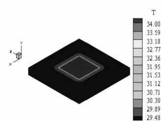
The material employed in this work is the Polyvinyl Chloride (PVC) with dimensions of 245 x 245 x 25 mm. The choice of PVC was due to the availability of samples of this material in the laboratory and the accurate knowledge of their thermal properties. The high values for the width and length of the sample are related with the insulation condition imposed in the theoretical model. It means that this condition needs to be reached for the success of the estimation techniques. A good way to reach the insulation condition in the horizontal direction is the use of a large sample. Since the method proposed in this work uses the frequency domain, it is necessary that the temperature signal, θ, goes to zero after heating. In this case, two thermocouples must be used and the difference between these temperatures must go to zero. When two thermocouples are used only on the upper surface, for non-conductive solid materials (in a two-dimensional or three-dimensional case), it is very difficult to obtain gradients with high enough values to allow any estimation (Fig. 3). To avoid this problem, thermocouples are placed here on the upper and lower surfaces. Figure 4 shows the sample temperature distribution that indicates a great gradient in the thickness direction.

Figure 4. Temperature evolution in the thickness of the sample.

Sensitivity Analysis

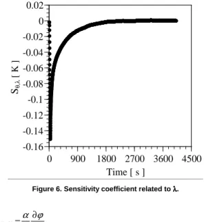
Another important way of analysis is to study the behavior of the sensitivity coefficients involved in the process. The first sensitivity coefficient analyzed is the Sϕ,α which is defined as the first derivative of the phase angle with respect to the α parameter (Eq. 12). Figure 5 shows the behavior of Sϕ,α in the frequency domain. It can be seen that for frequencies greater than 1.0 x 10-3 Hz, Sϕ,α becomes constant and little contribution is given to the estimation procedure. This fact reduces the analysis band and establishes the interest frequency in values less than 0.001 Hz. In this case, five representative points were used to determine α. The other important coefficient is related with λ in the time domain (Eq. 13). Figure 6 presents the Sθ,λcoefficient that is defined as the first derivative of the difference between the temperature model θ on the lower and upper surfaces, with respect to λ. The high values of this coefficient show the great advantage of thermal conductivity estimation in time domain. In Figure 6, for times greater than 1000 s, the sensitivity coefficient becomes negligible. In this work the sensitivity coefficients presented in Eqs. (12 and 13) are normalized in relation to α and λ, respectively.

Figure 5. Sensitivity coefficient related to αααα.

Figure 6. Sensitivity coefficient related to λλλλ.

, ,α _ϕα _αϕ ϕ = _∂∂

S (12)

. ) ( _{1 2}

2 1

,λ _θ λ_θ θ _λθ θ = ₋ ∂ _∂−

S (13)

Experimental Apparatus

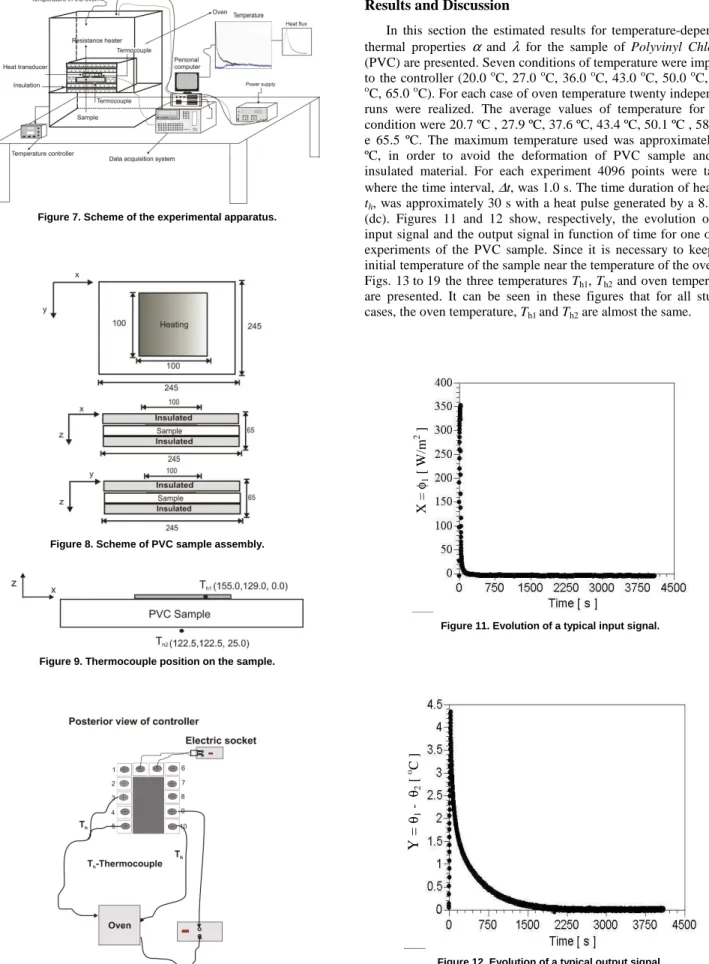
Figure 7 shows the experimental apparatus used to determine the thermal properties α and λ. A polymer sample of Polyvinyl Chloride (PVC) with thickness of 25 mm and lateral dimensions of 245 x 245 mm is used. These lateral dimensions are used in order to guarantee that the sample is submitted to a unidirectional and uniform heat flux on its upper surface, where at time t = 0 (T0), the sample is in thermal equilibrium. The heat is supplied by a 10.5 Ω electrical resistance heater, with lateral dimensions of 100 x 100 mm and thickness of 0.2 mm. The heat flux is acquired by a transducer with lateral dimensions of 50 x 50 mm, thickness of 0.2 mm, and constant time less than 10 ms. The transducer is based on the thermopile conception of multiple thermoelectric junction (made by electrolytic deposition) on a thin conductor sheet (Güths, 1994). In Figure 8 a detailed scheme of the PVC sample assembly is presented. The temperatures are measured using surface thermocouples (type T). The thermocouples disposition on the sample is shown in Fig. 9. The signals of heat flux and temperatures are acquired by a data acquisition system HP Series 75000 with the voltmeter E1326B controlled by a personal computer. The temperature in the oven was controlled by a PID temperature controller Watlow 93. Figure 10 presents how the controller was mounted to control the temperature in the oven. In this work seven temperature conditions are imposed to the controller.

Sϕ

,

α

[

r

ad

] •

• •

•• • • • • • • • • • • • • • • •

-0.4 -0.2 0 0.2

0 0.001 0.002 0.003 0.004 0.005

Frequency [ Hz ]

Sθ

,

λ

[

K

]

••••••• •• •• •• •• ••• ••• •••• •••• ••••• ••••••••• •••• ••••• •••••• ••••••••••••••••••••••••••••••••••• ••••••••••••••••••••••••••••••••••••••••••••••••••••••••••••

•••••••••••••••••••••••••••••••••••••••••••••••••••••••••••••••••••••••••••••••••••••••••••••••••••••••••••••••••••••••••••••••••••••••••• •••••••••••••••••••••••••••••••••••••••••••••••••••••••••••••••••••••••••••••••••••••••••••••••••••••••••••••••••••••••••••••••••••••••••••••••••••••••••••••••••••••••••••••••••••••••••••••••••••••••••••••••••••••••••••••••••••••••••••••••••••••••••••••••••••••••••••••••••••••••••••••••••••••••••••••••••••••••••••••••••••••••••••••••••••••••••••••••••••••••••••••••••••••••••••••••••••••••••••••••••••••••••••••••••••••••••••••••••••••••••••••••••••••••••••••••••••••••••••••••••••••

••••••••••••••••••••••••••••••••••••••••••••••••••••••••••••••••••••••••••••••••••••••••••••••••••••••••••••••••••••••••••••••••••••••••••••••••••••••••••••••••••••••••••••••••••••••••••••••••••••••••••••••••••••••••••••••••••••••••••••••••••••••••••••••••••••••••••••••••••••••••••••••••••••••••••••••••••••••••••••••••••••••••••••••••••••••••••••••••••••••••••••••••••••••••••••••••••••••••••••••••••••••••••••••••••••••••••••••••••••••••••••••••••••••••••••••••••••••••••••••••••••••••••••••••••••••••••••••••••••••••••••••••••••••••••••••••••••••••••••••••••••••••••••••••••••••••••••••••••••••••••••••••••••••••••••••••••••••••••••••••••••••••••••••••••••••••••••••••••••••••••••••••••••••••••••••••••••••••••••••••••••••••••••••••••••••••••••••••••••••••••••••••••••••••••••••••••••••••••••••••••••••••••••••••••••••••••••••••••••••••••••••••••••••••••••••••••••••••••••••••••••••••••••••••••••••••••••••••••••••••••••••••••••••••••••••••••••••••••••••••••••••••••••••••••••••••••••••••••••••••••••••••••••••••••••••••••••••••••••••••••••••••••••••••••••••••••••••••••••••••••••••••••••••••••••••••••••••••••••••••••••••••••••••••••••••••••••••••••••••••••••••••••••••••••••••••••••••••••••••••••••••••••••••••••••••••••••••••••••••••••••••••••••••••••••••••••••••••••••••••••••••••••••••••••••••••••••••••••••••••••••••••••••••••••••••••••••••••••••••••••••••••••••••••••••••••••••••••••••••••••••••••••••••••••••••••••••••••••••••••••••••••••••••••••••••••••••••••••••••••••••••••••••••••••••••••••••••••••••••••••••••••••••••••••••••••••••••••••••••••••••••••••••••••••••••••••••••••••••••••••••••••••••••••••••••••••••••••••••••••••••••••••••••••••••••••••••••••••••••••••••••••••••••••••••••••••••••••••••••••••••••••••••••••••••••••••••••••••••••••••••••••••••••••••••••••••••••••••••••••••••••••••••••••••••••••••••••••••••••••••••••••••••••••••••••••••••••••••••••••••••••••••••••••••••••••••••••••••••••••••••••••••••••••••••••••••••••••••••••••••••••••••••••••••••••••••••••••••••••••••••••••••••••••••••••••••••••••••••••••••••••••••••••••••••••••••••••••••••••••••••••••••••••••••••••••••••••••••••••••••••••••••••••••••••••••••••••••••••••••••••••••••••••••••••••••••••••••••••••••••••••••••••••••••••••••••••••••••••••••••••••••••••••••••••••••••••••••••••••••••••••••••••••••••••••••••••••••••••••••••••••••••••••••••••••••••••••••••••••••••••••••••••••••••••••••••••••••••••••••••••••••••••••••••••••••••••••••••••••••••••••••••••••••••••••••••••••••••••••••••••••••••••••••••••••••••••••••••••••••••••••••••••••••••••••••••••••••••••••••••••••••••••••••••••••••••••••••••••••••••••••••••••••••••••••••••••••••••••••••••••••••••••••••••••••••••••••••••••••••••••••••••••••••••••••••••••••••••••••••••••••••••••••••••••••••••••••••••••••••••••••••••••••••••••••••••••••••••••••••••••••••••••••••••••••••••••••••••••••••••••••••••••••••••••••••••••••••••••••••••••••••••••••••••••••••••••••••••••••••••••••••••••••••••••••••••••••••••••••••••••••••••••••••••••••••••••••••••••••••••••••••••••••••••••••••••••••••••••••••••••••••••••••••••••••••••••••••••••••••••••••••••••••••••••••••••••••••••••••••••••••••••••••••••••••••••••••••••••••••••••••••••••••••••••••••••••••••••••••••••••••••••••••••••••••••••••••••••••••••••••••••••••••••••••••••••••••••••••••••••••••••••••••••••••••••••••••••••••••••

-0.16 -0.14 -0.12 -0.1 -0.08 -0.06 -0.04 -0.02 0 0.02

0 900 1800 2700 3600 4500

Figure 7. Scheme of the experimental apparatus.

Figure 8. Scheme of PVC sample assembly.

Figure 9. Thermocouple position on the sample.

Figure 10. Scheme representation of the controller.

Results and Discussion

In this section the estimated results for temperature-dependent thermal properties α and λ for the sample of Polyvinyl Chloride (PVC) are presented. Seven conditions of temperature were imposed to the controller (20.0 o_{C, 27.0} o_{C, 36.0} o_{C, 43.0} o_{C, 50.0} o_{C, 58.0} o

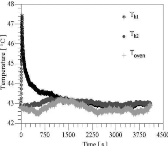
C, 65.0 oC). For each case of oven temperature twenty independent runs were realized. The average values of temperature for each condition were 20.7 ºC , 27.9 ºC, 37.6 ºC, 43.4 ºC, 50.1 ºC , 58.0 ºC e 65.5 ºC. The maximum temperature used was approximately 70 ºC, in order to avoid the deformation of PVC sample and the insulated material. For each experiment 4096 points were taken, where the time interval, ∆t, was 1.0 s. The time duration of heating, th, was approximately 30 s with a heat pulse generated by a 8.50 V (dc). Figures 11 and 12 show, respectively, the evolution of the input signal and the output signal in function of time for one of the experiments of the PVC sample. Since it is necessary to keep the initial temperature of the sample near the temperature of the oven, in Figs. 13 to 19 the three temperatures Th1, Th2 and oven temperature are presented. It can be seen in these figures that for all studied cases, the oven temperature, Th1 and Th2 are almost the same.

Figure 11. Evolution of a typical input signal.

Figure 12. Evolution of a typical output signal.

Y

=

θ1

θ2

[

o C

]

X

=

φ1

[

W

/m

Figure 13. Experimental temperatures for the case of average temperature 20.7 oC.

Figure 14. Experimental temperatures for the case of average temperature 27.9 oC.

Figure 15. Experimental temperatures for the case of average temperature 37.6 o C.

Figure 16. Experimental temperatures for the case of average temperature 43.4 oC.

Figure 17. Experimental temperatures for the case of average temperature 50.1 o C.

Figure 19. Experimental temperatures for the case of average temperature 65.5 o C.

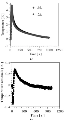
In Figure 20a, a comparison between estimated and experimental phase factor is presented. It can be observed a very good agreement. Figure 20b shows the residuals. A comparison between estimated and experimental temperatures for α = 1.26 x 10-07 m2/s and λ = 0.161 W/m.K of one experiment (oven temperature 27.9 o_{C) is shown in Fig. 21a. Again, a good agreement} between the data can be observed. It can be noted that the residuals presented in Fig. 21b are situated in the range of uncertainty measurement of thermocouples, which in this work is ± 0.3 K. For the other cases of oven temperature the results for the estimated and experimental phase and the temperature presented the same behavior. For all cases the differences were smaller than 5 %.

ϕe

ϕt

ϕ

[

ra

d

]

a)

b)

Figure 20. Phase factor: a) experimental and calculated data b) residuals.

∆θe

∆θt

a)

••••••••••••••

••••

••••••••••

_{••••••••}

•••••••

•

••

••

••

••

•••

••••••

••••••••••••••••••••••••••••••••••••••••••••••••••••••••••••••••••••••••••••••••••••••••••••••••••••••••••••••••

•••••••••••••••••••••••••••••••••••••••••••••••••••••••••••••••••••••••••••••••••••••••••••••••••••••••••••••••••••••••••••••••••••••••••••••••••••••••••••••••••••••••

_{••••••••••••••••••••••••••••••••••••••••••••••••••••••••••••••••••••••••••••••••••••••••••••••••••••••••••••••••••••••••••••••••••••••••••••••••••••••••••••••••••••••••••••••••••••••••••••••••••••••••••••••••••••••••••••••••••••••••••••••••••••••••••••••••••••••••••••••••••••••••••••••••••••••••••••••••••••••••••••••••••••••••••••••••••••••••••••••••••••••••••••••••••••••••••••••••••••••••••••••••••••••••••••••••••••••••••••••••••••••••••••••••••••••••••••••••••••••••••••••••••••••••••••••••••••••••••••••••••••••••••••••••••••••••••••••••••••••••••••••••••••••••••••••••••••••••••••••••••••••••••••••••••••••••••••••••••••••••••••••••••••••••••••••••••••••••••••••••••••••••••••}

-0.4 -0.2 0 0.2 0.4

0 300 600 900 1200

T

e

m

p

e

ra

tu

re

r

e

si

d

u

a

ls

[

K

]

Time [ s ] b)

Figure 21. Temperature evolution: a) experimental and calculated data b) residual.

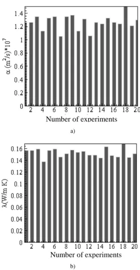
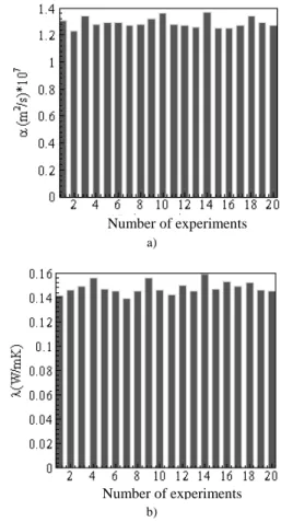
Figures 22 to 28 present the values obtained for α and λ for all cases studied of average temperature. When analyzing a series of measurements some data can present uncertainties that interfere in the process, causing inexact values. The causes of these uncertainties are many. In the case of thermal properties determination, the most common ones are: errors in the restrictions of the theoretical model, errors in temperature and heat flux measurements due to calibration, time response, thermal contact resistance in the sensors and measurement uncertainty in the data acquisition of the signals. A tool extensively used to decide the rebound of data is the Chauvenet’s criterion (Taylor, 1997). The use of this criterion allows that medium values of α and λ to be obtained using a confidence interval of 99 %.

Number of experiments a)

Number of experiments b)

Figure 22. (Continued).

Number of experiments a)

Number of experiments b)

Figure 23. Histogram of a) αααα and b) λλλλ for the average temperature 27.9 o C.

Number of experiments a)

Number of experiments b)

Figure 24. Histogram of a) αααα and b) λλλλ for the average temperature 37.6 o C.

a)

b)

Figure 25. Histogram of a) αααα and b) λλλλ for the average temperature 43.4 oC. Number of experiments

a)

b)

Figure 26. Histogram of a) αααα and b) λλλλ for the average temperature 50.1 °C.

Number of experiments

a)

Number of experiments

b)

Figure 27. Histogram of a) αααα and b) λλλλ for the average temperature 58.0 oC.

a)

b)

Figure 28. Histogram of a) αααα and b) λλλλ for the average temperature 65.5 oC.

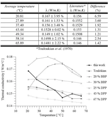
Tables 1 and 2 present respectively the estimated mean values for α and λ. In this work, for each averaged temperature analyzed, 20 experiments were carried out. Only the reference value of α for the room temperature of 27.9 ºC was found (Table 1). This value was obtained by using the Flash method (Lima e Silva et al., 2003). The values used in Table 2 for λ are referred to curve 7 (Touloukian et al., 1970). For the thermal conductivity, the estimated values for all cases of average temperature were compared with the reference Touloukian et al. (1970) (Fig. 29). In Figure 29, a comparison with other curves obtained from the literature Technology of Plasticizers (Sears and Darby, 1982) is also presented. In this reference, each curve presents different compositions of plasticizer concentration.

Table 1. Statistic data for the average values estimated for αααα of the PVC sample.

Average

temperature (ºC) α(m2/s) x 1007

Literature*

α(m2_{/s) x 10}07 _{Difference (%)} 20.81 1.30 ± 3.18 % __

27.89 1.26 ± 2.88 % 1.28 1.59 37.40 1.29 ± 3.81 % __ __ 43.44 1.28 ± 5.38 % __ __ 49.34 1.28 ± 1.74 % __ __ 58.14 1.29 ± 1.82 % __ __ 65.89 1.29 ± 1.86 % __ __

* Lima e Silva et al. (2003)

It can be observed, in Fig. 29, that the majority of curves presents the same behavior, i.e., the thermal conductivity decreases with the temperature increase. This thermal conductivity decline can be explained by the sample dilation, due to the increase of the

Number of experiments Number of experiments

temperature. Although, this dilation is visually very small, it causes a considerable change in the properties of the sample. It can not be assured that the sample used here has the same compositions of those of plasticizer content and molecular weight. However, to guarantee more reliable results, the value of the thermal conductivity obtained in this work, in the temperature of 27 ºC, was compared with the result λ = 0.16 W/m.K, obtained from IPT (2004). In this case, the same sample was measured at room temperature using the guarded hot plate method by IPT (2004). The difference was less than 3.0 %.

Table 2. Statistic data for the average values estimated for λλλλ of the PVC sample.

Average temperature

(ºC) λ(W/m.K)

Literature*

λ(W/m.K)

Difference (%)

20.81 0.167 ± 3.95 % 0.156 6.59 27.89 0.161 ± 1.53 % 0.1552 3.60 37.40 0.156 ± 3.48 % 0.1529 1.92 43.44 0.1528 ± 0.02 % 0.153 1.31 49.34 0.149 ± 1.02 % 0.1508 1.21 58.14 0.1498 ± 2.15 % 0.146 2.54 65.89 0.1481 ± 2.22 % 0.146 1.42

*Touloukian et al. (1970)

Figure 29. Comparison of the results for the thermal conductivity.

Conclusions

In this work, a Polyvinyl Chloride sample was exposed to different temperatures inside an oven and the thermal properties were estimated with an additional heating relative to a temperature difference of approximately 4.5 °C. This process was necessary to identify the thermal properties in a representative average temperature. The technique based on the use of an input/output dynamical system shows to be suitable to be applied to determine temperature-dependent thermal properties. It can be observed that the results present good agreement with the respective reference values. This technique can also be used for conductor applications.

Acknowledgements

The authors would like to thank CAPES, CNPq (Proc. 470253/2006-1) and FAPEMIG (TEC 1928/06, 0084/06 and 00144/08), Government Agencies, for the financial support without which this work would not be possible. They are also grateful to

Eng. Cleber Spode and the Technician Lázaro Henrique A. Vieira for technical support.

References

Alifanov, O.M., 1974, “Solution of an Inverse Problem of Heat Conduction by Iteration Methods”, Journal of Engineering Physics, Vol. 26,

No. 4, pp. 471-476.

Beck, J.V., Blackwell, B. and St. Clair, C., 1985, “Inverse Heat Conduction: Ill-posed Problems”, Wiley-Interscience Publication, New York, 326 p.

Bendat, J.S. and Piersol, A.G., 1986, “Analysis and Measurement

Procedures”, Wiley-Interscience, 2° Ed., USA, 566 p.

Blackwell, J.H., 1954, “A Transient-Flow Method for Determination of Thermal Constants for Insulating Materials in Bulk”, Journal of Applied Physics, Vol. 25, No. 2, pp. 137-144.

Borges, V.L., Lima e Silva, S.M.M. and Guimarães, G., 2006, “A Dynamic Thermal Identification Method Applied to Conductor and Non Conductor Materials”, Inverse Problems in Science & Engineering, Vol. 14,

No. 5, pp. 511-527.

Chantasiriwan, S., 2002, “Steady-State Determination of Temperature-Dependent Thermal Conductivity”, Int. Comm. Heat Mass Transfer, Vol. 29,

No. 6, pp. 811-819.

Dowding, J.K., Beck, J.V. and Blackwell, B.F., 1999, “Estimating Temperature-Dependent Thermal Properties”, Journal of Thermophysics and Heat Transfer, Vol. 13, No. 3, pp. 328-336.

Defer, D., Antczak, E. and Duthoit, B., 1998, “The Characterization of Thermophysical Properties by Thermal Impedance Measurements Taken Under Random Stimuli Taking Sensor-Induced Disturbance Into Account”,

Meas. Sci. Technol., Vol. 9, No. 3, pp. 496-504.

Eriksson, R., Hayashi, M. and Seetharaman, S., 2002, “Thermal Diffusivity Measurements of Liquid Silicate Melts”, The Sixteenth European Conference for Thermophysical Properties (ECTP2002), London, UK.

Güths, S., 1994, “Anémomètre a Effet Peltier et Fluxmètre Thermique: Conception et Réalisation”. Application à l’etude de la Convection Naturelle, Thèse de Doctorat, Université d’Artois, France.

IPT, Instituto de Pesquisas Tecnológicas, 2004, “Determinação de Condutividade Térmica”, Relatório de ensaio nº. 908637, fevereiro.

Kim, S., Lee, K.J., Ko, Y.J., Kim, M.C. and Kim, K.Y., 2004, “Estimation of Temperature-Dependent Thermal Conductivity and Heat Capacity Per Unit Volume With a Simple Integral Approach”, Int. Comm. Heat Mass Transfer, Vol. 31, No. 7, pp. 981-990.

Lima e Silva, S.M.M., Ong, T.H. and Guimarães, G, 2003, “Thermal Properties Estimation of Polymers Using Only One Active Surface”, J. of the Braz. Soc. Mechanical Sciences, Vol. XXV, No. 9, pp. 9-14.

Luo, D., He, L., Lin, S., Chen, T.F. and Gao, D., 2003, “Determination of Temperature Dependent Thermal Conductivity by Solving IHCP in Infinite Region”, Int. Comm. Heat Mass Transfer, Vol.30, No.7, pp. 903-908.

Mardolcar, U. V., 2002, “Thermal Diffusivity of Rocks at High Temperature by the Laser Flash Technique”, The Sixteenth European Conference for Thermophysical Properties (ECTP2002), London, UK

Miyamura, A. and Susa, M., 2002, “Relative Measurements of Thermal Conductivity of Liquid Gallium by Transient Hot Wire Method”, The Sixteenth European Conference for Thermophysical Properties (ECTP2002), London, UK.

Parker, W.J., Jenkins, R.J., Butler, C.P. and Abbott, G.L., 1961, “Flash Method of Determining Thermal Diffusivity, Heat Capacity and Thermal Conductivity“, Journal of Applied Physics, Vol. 32, pp. 1679-1684.

Santos, W.N., Mummery, P. and Wallwork, A., 2005, “Thermal Diffusivity of Polymers by the Laser Flash Technique”, Polymer Testing,

Vol. 24, No. 5, pp. 628-634.

Sears, J.K. and Darby, J.R., 1982, “Technology of Plasticizers”, John Wiley & Sons Inc, 1180 p.

Taylor, J.R., 1997, “An Introduction to Error Analysis: The Study of Uncertainties in Physical Measurements”, University Science Books, 2nd _ed.,

327 p.

Touloukian, Y.S., Powell, R.W., Ho, C.Y. and Klemens, P.G., 1970, “Thermophysical Properties of Matter”, Thermal Conductivity: Nonmetallic Solids, IFI/Plenum, New York, Vol. 2, 933 p.