Lat. Am. j. solids struct. vol.13 número9

Abstract

This study is devoted to strain-based formulation for a curved beam. Arches with parabolic geometry, which have a variety of applications, belong to this structural type. Dependency of the curvature radius to the arch length creates some complexities in the solution process. To analyze these complex structures, a two-node beam with six degrees of freedom is suggested by utilizing closed-form solution and the stiffness-based finite element method. Considering the effect of shear deformation, and incorporating equilibrium conditions into the finite element model, lead to the exact strains. Displacements and explicit stiffness matrix are found based on these exact strains. To validate the efficiency of the author's formulation, seven numerical tests are performed. The outcomes demonstrate that by employing only a single element, the locking-free answers can be found.

Keywords

Finite element method, parabolic beam, explicit stiffness matrix, strain-based formulation, equilibrium conditions.

An Explicit Stiffness Matrix for Parabolic Beam Element

1 INTRODUCTION

For many years, researchers used a lot of short straight beams to analyze curved structures Kikuchi (1975) Kikuchi and Tanizawa (1984) Chapelle (1997). In spite of the simple process, solving arches by implementing these elements, even by reducing the mesh sizes, faces some troubles and complex-ities. This kind of modeling for thin members leads to excessive stiff behavior and causes shear lock-ing phenomena. To remove these errors, investigators have formulated these beams with curved geometry. At first, by utilizing interpolation functions, with the same order and having independent terms, displacement-based elements were proposed. These models resulted in responses with locking errors. To overcome this obstacle, the number of nodes and order of functions were increased Ashwell and Sabir (1971) Dawe (1974) Meck (1980). Reduced integration assumed strain function and hybrid-mixed formulation are the other methods for creating locking-free elements Stolarski and Belytschko (1982) Pandian et al. (1989) Choi and Lim (1993 and 1995) Yang and Sin (1995) Kim and Park (2008) Benedetti and Tralli (1989) Kim and Kim (1998) Kim and Lee (2008).

Mohammad Rezaiee-Pajand a Niloofar Rajabzadeh-Safaei b

a _{Civil Engineering, Ferdowsi University} of Mashhad, Iran, Tel/fax: +98-51-38412912, (Professor) Email: re-zaiee@um.ac.ir

b _{Structural Engineering, Ferdowsi} Uni-versity of Mashhad, Iran, (Graduate student) Email:

niloofarsa-faee@gmail.com

http://dx.doi.org/10.1590/1679-78252820

Raveendranath and his colleagues (1999) assumed cubic polynomial for radial displacement. By taking advantage of the equilibrium equations, they suggested new displacement functions Raveendranath et al. (2001). Similarly, this procedure was extended to create a three-nodded ele-ment. Furthermore, it was stated that the consistent-field approach can find the sources of high-stiffening errors. Afterward, many formulations were presented based on this effective technique Babu and Prathap (1995) Prathap and Naganarayana (1990).

All mentioned investigators studied about curved beams with the constant radius of curvature. In addition, few papers have focused on the variable-curvature structures. Marquis and Wang (1989) used the energy principles to solve parabolic arches. It is worth emphasizing that most of the proposed schemes have not offered a general finite element model. In fact, these solution techniques have only considered a few particular cases that were more reachable. These investigators calculated the stiffness matrix by considering the effect of special boundary conditions Gutierrez et al. (1989) Lin and Huang (2007) Lin and Hsieh (2007) Lee and Wilson (1989) Lee et al. (2008) Tarnopolskaya et al. (1996). Haung et al. (1998) utilized polynomial functions and power series to model the be-havior of beams with variable curvatures and cross sections. In 1999, Oh et al. (1999) solved equi-librium equations numerically, and found the first four natural frequencies of sinusoidal, elliptical and parabolic beams for the special cases. This procedure was used by many researchers Huang et al. (1998) Oh et al. (2000) Gimena et al. (2010). Another way of finding the structural stiffness matrix is the flexibility-based method. Litewka and Rakowski (1998), Molari and Ubertini (2006), and Attarnejad et al. (2013) utilized this approach in their study. Attarnejad and his coworkers (2013) defined Basic Displacement Function (BDF) as the nodal displacement by applying unit load technique. On the other hand, Molar & Ubertini (2006) employed a parametric cubic interpolation to model geometry of the structure. These investigators considered two parameters for the versatili-ty of interpolation function.

In this research, a scheme for analyzing general curved beam with the variable curvature is sug-gested. Parabolic shapes are widely used in the group of arches, for their simple second-order poly-nomial form. By employing the finite element method and closed-form solution, a novel parabolic beam element is proposed. Choosing required interpolation function and satisfying the equilibrium conditions have the most significant role in this procedure. In fact, by employing just one element per member, precise responses are found. This is due to the exact strains that obtained by solving differential equations. Moreover, an explicit stiffness matrix is obtained, which can be used in the structural analysis. It should be noted that all shear, axial and bending effects are considered, sim-ultaneously. The results of seven numerical tests show no locking error in the answers. All entries of the suggested stiffness matrix are explicitly given in the appendix.

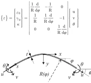
2 EQUILIBRIUM EQUATIONS

assumed as w and t. It should be noted that the geometry of suggested element is based on the

sec-ond-order polynomial function. Using the equations_{y =a x.} 2 _{+b x. +c,}

3 2 2

1

(1 )

y R

y ¢¢ =

¢ + andy¢ = tanj, the radius of curvature function, R, can be achieved. In these formulas, φ denotes the angle of tangential slope at a general point.

R = 0

0 3

1

( ) ,

2 cos

R

R R

a

j

j

= = ₍₁₎

Strain functions for the neutral axis have the following form:

{ }

φ

φ

θ φ 0

0

1 d 1

0

R d R _u

1 1 d

1 v

R R d

1 d

0 0

R d

e

e g

k

é ù

ê - ú

ê ú

ì ü ì ü

ï ï _{ê ú}ï ï

ï ï ï ï

ï ï ê úï ï

ï ï ï ï

=í ý_{ï ï}=ê_ê - ú_úí_ï ý_ï

ï ï _{ê ú}ï ï

ï ï ï ï

ï ï ï ï

î þ ê_ê ú_úî þ

ê ú

ë û

(2)

Figure 1:Geometry of a parabolic beam.

By integrating the stresses over the thickness of cross section, the compliance material matrix can be found. If the effect of thickness in strain equations is negligible, the following simple and approximate material matrix will be obtained:

é ù

ê ú

ê ú

é _{ù = ê ú}

ë û _{ê ú}

ê ú

ê ú

ë û

m

EA

0

0

D

0

kGA

0

0

0

EI

(3)

Approximate material matrix is based on the assumption of t/R<<1. Furthermore, the first three terms of Taylor's series are utilized for ln(2R t)

2R t

+

- and the membrane-bending interaction is eliminated. With these assumptions andε 1σ

m

D - .

0 x 0 y z 1 0 0 EA N 1

0 0 V

M 1 0 0 EI kGA e g k é ù ê ú ê ú

ì ü ì ü

ï ï ï ï

ï ï ê úï ï

ï ï _{ê ú}ï ï

ï ï₌ ï ï

í ý ê úí ý

ï ï _{ê ú}ï ï

ï ï ï ï

ï ï _{ê ú}ï ï

ï ï ï ï

î þ _{ê ú}î þ

ê ú

ë û

(4)

The Young’s modulus, shear modulus, area of the cross-section, bending moment of inertia about the neutral axis, and a shear correction factor are indicated as E, G, A, I, k, respectively. A set of equilibrium equations can be achieved by optimization of the following total potential energy:

0

d = ¾¾

y x,s x y,s z,s y V 0 N R N 0 V R V 0 M ìïï

ï - =

ïï ïï

ï _{+ =}

íï

ïï _{+ =}

ïï ïï ïî

(5)

In these equations, subscript s demonstrates the differentiating with respect to the longitudinal axis s. The related answers for the set of equilibrium equations can be written in the below form:

x 1 2

y 1 2

z 1 1 2 2 3

c .cos c .sin N

c .sin c .cos V

ˆ ˆ

c .C .C

M c c

j j

j j

ìï _{= - +}

ïï

ï _{= +}

íï

ïï = + +

ïî

(6)

The unknowns

C

1

ˆ

_and

2

C

ˆ

_{are expressed as:}

ìï ₌ ïï íï = ïïî

ò

ò

1 2

ˆ _{( ).sin .}

ˆ _{( ).cos .}

C R d

C R d

j j j

j j j (7)

3 DISPLACEMENT FUNCTIONS

By assuming t/R<<1, the membrane-bending interaction is omitted. Consequently, internal forces cause the next strains in the neutral axis.

0 1 2

0 1 2

1 2

1 2 3

cos sin

. .

sin cos

. .

ˆ ˆ ₁

. . . c c AE AE c c kGA kGA C C

c c c

j j

e

j j

g

k

ìï æ- ö æ ö

ï ç ÷ ç ÷

ï = ç ÷ +_÷ ç ÷_÷

ï ç_è ÷_ø ç_è ÷_ø

ïï

ï _{æ ö æ ö}

ïï ₌ ç ÷_{÷ +} ç ÷_÷

í ç_{ç ÷÷} ç_{ç ÷÷}

ï è ø è ø

ïï _{æ ö æ ö}

ï _{÷ ÷} æ ö

ï ç ÷ ç ÷ ç ÷

ï = ç ÷+ ç ÷+ ç ÷÷

ï çç ÷÷ çç ÷÷ ç ÷

ï è ø

, 0 0, , 0 0

, R. .d

u u R( ) .

v u R.

R

jj j j

j

q k j

g q e e

e

ìï = ïï

ïï + = + + +

íï

ïï =

-ïïî

ò

(9)

Then, the coming displacement fields can be found by solving the equilibrium equations:

1 1 2 2 3 3 1 1 2 3

1 1, 2 2, 3 3,

1 1, 2 3

1 1 2 2 3 3 1

( ) . . . . ' . sin . cos

. cos . sin

v( ) . . .( )

. .cos . sin

( ) . . .

u c C c C c C d D d d

R R

c C c C c C

AE AE

d D d d

c C c C c C d

j j j

j

j j j

j j

j

j j

q j

ì = ¢¢+ ¢¢+ ¢¢+ + +

ïï

ïï æ ö æ ö

ï ç _¢¢ ÷ ç _¢¢ ÷ _¢¢

ï = ç + ÷ +_÷ ç - ÷ +_÷

ï ç_è ÷_ø ç_è ÷_ø

íï

ï+ ¢ +

-ïï

ï _{¢ ¢ ¢}

ï = + + +

ïî (10) 1 1 2 2 3 ˆ . . ˆ . . . C

C R d

EI C

C R d

EI R C d EI j j j

ì æ ö

ï _{ç ÷}

ï _{¢ = ç ÷}

ï _ç ÷

ï _{çè ÷÷ø}

ïï

ï _{æ ö}

ï _{ç ÷}

ï _{¢ = ç ÷}

í _ç ÷_÷

ï _çè ÷_ø

ïï ïï ¢ ï = ïï ïî

ò

ò

ò

(11)

1 1 ,

1 ,

2 2 ,

. sin . sin cos

sin . cos . . . .

. sin . sin cos

cos . sin . . . .

. cos . cos sin

sin . cos . . .

R R

C R C R d

kGA AE AE

R R

R C R d

kGA AE AE

R R

C R C R

kGA AE

j

j

j

j j j

j j j

j j j

j j j

j j j

j j

æ æ- öö_÷÷

ç ç

¢¢= ç_ç + ¢+ + ç_ç ÷÷_÷÷÷÷

è è øø

æ æ_- öö_÷÷

ç _¢ ç

+ - ç_ç + + + ç_ç ÷÷_÷÷÷÷

è è øø

¢¢= + ¢ + +

ò

ò

ò

2 , 3 3 3 1 .

. cos . cos sin

cos . sin . . . .

sin . cos .( . ).

cos . sin .( . ).

' sin . . cos . cos . . sin .

d AE

R R

R C R d

kGA AE AE

C R C d

R C d

D R d R d

j

j

j j j

j j j

j j j

j j j

j j j j j j

ìïï ïï ïï ïï ïï ïï

ï _{æ æ öö÷÷}

ç ç _÷÷

ç ç _÷÷

ç ç ÷÷

è è øø

í _{æ æ öö}

÷÷

ç ¢ ç

+ - ç_ç + + + ç_ç ÷÷_÷÷÷÷

è è øø

¢¢= ¢ ¢ + -= +

-ò

ò

ò

ò

ò

ïï ïïï ïï ïï ïï ïï ïï ïï ïï ïï ïïî (12)

Furthermore, the vector of nodal unknowns is obtained as bellow:

T

1 2 3 1 2 3

ˆ = êé_ëc c c d d d ù_úû

q ₍₁₃₎

Finally, the next strain and displacement interpolation functions can be derived:

q .ˆ

q

0 0

2

1 1

.cos .sin 0 0 0 0

EA EA

1 1

B .sin .cos 0 0 0 0

kGA kGA

R 1 R 1

. .(-tan ) 0 0 0

EI 2. cos EI EI

j j

j j

j j

é ù

ê _- ú

ê ú

ê ú

ê ú

é _{ù = ê ú}

ë û _{ê ú}

ê æ_{ç -} ö_÷ ú

ê _{ç ÷÷} ú

ê ç_çè ÷_ø ú

ê ú

ë û

(15)

2 2

0 0

3 2 4 2 2

0

5

0

q

sin cos .ln(sec tan ) sin cos .ln(sec tan )

1

kGA 2 cos EA cos

(105 cos 90)cos .ln(sec tan ) sin .cos .(105 cos 20) 4 sin

,

EI 960 cos

1 kGA 2 N R R R R

j j j j j j j j

j j

j j j j j j j j

j

æ _{+ +} ö_÷ æ _{+ +} ö_÷

ç _÷ ç _÷

ç _÷+ ç- _÷

ç ÷÷ ç ÷÷

ç ç

è ø è ø

æ _{- + + - -} ö_÷

ç _÷

ç

+ _{ç ÷÷÷}

çè ø

é _{ù =} ë û

2 2

0 2

3 2 4 2 4 2

0

6

2 0

4

cos 1 sin .cos .ln(sec tan )

( 1 sin .ln(sec tan ))

EA cos

(105 cos 90)sin .cos .ln(sec tan ) cos .( 105 cos 44 55 cos ) 20

,

EI 960 cos

sin 3.sin . EI 8.cos R R R

j j j j j

j j j

j

j j j j j j j j

j

j j

j

æ _{+ - +} ö_÷

ç _÷

ç _÷+ - + +

ç _÷÷

çè ø

æ _{+ + + - + - +} ö_÷

ç _÷

ç

- _{ç ÷÷÷}

çè ø

-

-2 3

.ln(sec tan ) , 16

16.cos j j j

é ê ê ê ê ê ê ê ê ê ê ê ê ê ê ê ê

ê æ_{ç ö÷}

ê _{ç - + ÷÷}

ê ç_çè ÷_ø

ê ê ê ê êë

(

)

2 2

0 0

2

3 4 2 2

0

4 2

0

cos 1 sin .cos . ln(sec tan )

1 1 sin . ln(sec tan )

kGA EA 2 cos

15 sin .cos .ln(sec tan ) 5 cos .(1 3 cos ) 2 ,

EI 120 cos

sin cos .ln(sec tan )

kGA cos

R R

R

R

j j j j j

j j j

j

j j j j j j

j

j j j j

j

æ _{+ - +} ö_÷

ç _÷

ç

- + + + _{ç ÷}

÷÷

çè ø

æ _{+ + - + ÷}ö

ç _÷

ç

+ _ç- _÷÷÷

çè ø

æ _{+ +} ö_÷

çç

ççè ø

2 0

2

3 6 2 4

0

5 2 0

3

sin cos . ln(sec tan )

1

EA 2 cos

15 cos . ln(sec tan ) sin .(8 10 cos 15 cos ) ,

EI 120 cos

1

. ,

EI 3. cos

R

R

R

j j j j

j

j j j j j j

j

j

æ _{+ +} ö_÷

ç

÷+ ç- ÷

÷ _ç ÷

÷ ÷

÷ _çè ÷_ø

æ _{+ + + +} ö_÷

ç _÷

ç

+ _ç- _÷÷÷

çè ø

æ _- ö_÷

ç _÷

ç _÷

ç ÷

çè ø

2 2 2 2

0

3

2 2 2 2 2

0

4 2 0

2

(15 cos 12).cos .ln(sec tan ) 15 sin .cos 2 sin ,

EI 48 cos

(15 cos 12) sin .cos .ln(sec tan ) 6 cos .(15 cos 7)

,

EI 48 cos

sin cos .ln(sec tan )

.

EI 2. cos

R

R

R

j j j j j j j

j

j j j j j j j

j

j j j j

j

æ _{- + + -} ö_÷

ç _÷

ç- _÷

ç _÷÷

çè ø

æ _{+ + + - +} ö_÷

ç _÷

ç _÷

ç _÷÷

çè ø

æ _{+ +}

çç

è ö÷÷÷,

ç _÷÷ ç _ø 2 0 2 0 2

1 2 cos

sin cos

2 cos

sin .(1 2 cos )

cos sin

2 cos

1 0 0

R R j j j j j j j j j

æ _- ö_÷ ù

ç ÷ ú

ç _÷

ç _÷÷ ú

çè ø _ú

ú

æ ₊ ö_÷

ç _÷ ú

ç _÷ - _ú

ç _÷÷

çè ø ú

ú ú ú

4 FINITE ELEMENT FORMULATION

If

φ

is inserted in the equation (16), the vector of the nodal displacement will be found. It should be noted,

φ

for the first node is zero while for the second one is unknown. The structural geometry is utilized to find the amount of

φ

.

q

ˆ _{= ê ú}é ù _.ˆ

ë û

D G q

,

DˆT = ê_ëéu₁ v₁ q₁ u₂ v₂ q₂ù_úû (17)

q ˆ

ˆ_{= ê ú}é_ë ù_û-1

q G .D (18)

At first, the displacement and strain interpolation functions are determined according to the vector of nodal displacements. Then, the following shape functions become available:

-1

u = _ëéN_{qû ë}ù.(_êéG_qúûù .Dˆ)

,

e = é_ëB_qù_{û ë}.(_êéG_qù_ûú-1 .Dˆ) (19)

q q

ˆ ₌ é_ë ù_{û ë}é_ê ù_ú û

-1

N N . G , Bˆ= é_ëB_qù_{û ë}. Gé_{ê q}ù_úû-1 (20)

Total potential energy can be written in terms of the strain interpolation function:

T

u F u .{P

T T

m i i

i 1,2 1

{ } . D .{ }.ds - { } .{ }.ds { } }

s s

2 e e

=

é ù

 =

_ò

_{ë û}

_ò

-

å

₍₂₁₎

By optimization Π, a general finite element formulation is obtained for each member:

B T _m B Dˆ N T F P_{i i 1,2}

( . D . .ds). .{ }.ds { }

sé ù éë û ë ù é ùû ë û = sé ùë û + =

ò

ò

(22)

S D.ˆ { }P

é ù =

ë û

S B B

P N F P

T m T

i i 1,2

. D . .ds

s

{ } .{ }.ds { }

s =

ìï é ù ₌ é ù é ù é ù

ï _{ë û ë û ë û ë û}

ïïí

ï _{= é ù +}

ï _{ë û}

ïïî

ò

ò

(23)

Calculating the exact integration over the arch length leads to the precise elemental stiffness matrix. It should be added that general form of the stiffness matrix entries,

S

ij, are based on the

approximation of the compliance material matrix. All of these entries are explicitly given in the appendix.

5 NUMERICAL STUDIES

5.1 A Two-End Fixed Beam

A beam with a radial load at its middle point and two fixed supports is shown in Figure 2. Elastici-ty modulus of Young, thickness and radius of curvature are 30,000( k/in2), 6( in) and 1200 (in), respectively. Also, the tangent angle of the beam end is _α =11.31° . Figure 2, illustrates the geome-try of structure. Due to symmegeome-try, this arch can be modeled with a single element. Marquis and Wang (1989) analyzed parabolic beams by taking advantage of potential energy principles. In this section, the answers of the proposed method can be compared with the responses of their study. It should be noted that they ignored the shear effect to solve this structure. The obtained results are available in Table 1.

Figure 2: Geometry of a two-end fixed parabolic beam Marquis and Wang (1989).

Present method with no shear effect Marquis and Wang (1989) with no

shear effect

1.2309E-03 1.2309E-03

Table 1: Middle point radial displacement of a two-end fixed beam with a central radial load.

According to the results, there is no locking error in the answers of the suggested element.

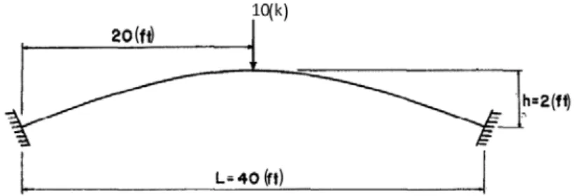
5.2 Verifying Responses

Exact Present method

Slender-ness ratio

 

R₀ t

Structural geometry θc vc uc θ v u -6.0156E-08 0.0000 4.7428E-07 -6.0156E-08 0.0000 4.7428E-07 5 -6.4613E-05 0.0000 2.1447E-04 -6.4613E-05 0.0000 2.1447E-04 50 -5.1717E-04 0.0000 1.7000E-03 -5.1717E-04 0.0000 1.7000E-03 100 0.0000 1.3525E-06 0.0000 0.0000 1.3525E-06 0.0000 5 0.0000 3.1481E-04 0.0000 0.0000 3.1481E-04 0.0000 50 0.0000 2.4527E-03 0.0000 0.0000 2.4527E-03 0.0000 100 3.2872E-08 0.0000 -6.0156E-08 3.2872E-08 0.0000 -6.0156E-08 5 3.1426E-05 0.0000 -6.4613E-05 3.1426E-05 0.0000 -6.4613E-05 50 2.5132E-04 0.0000 -5.1717E-04 2.5132E-04 0.0000 -5.1717E-04 100 -3.0596E-08 0.0000 3.3241E-07 -3.0596E-08 0.0000 3.3241E-07 5 -3.3000E-05 0.0000 8.4414E-05 -3.3000E-05 0.0000 8.4414E-05 50 -2.6406E-04 0.0000 6.6028E-04 -2.6406E-04 0.0000 6.6028E-04 100 0.0000 1.3414E-06 0.0000 0.0000 1.3414E-06 0.0000 5 0.0000 2.1845E-04 0.0000 0.0000 2.1845E-04 0.0000 50 0.0000 1.6618E-03 0.0000 0.0000 1.6618E-03 0.0000 100 2.6714E-08 0.0000 -3.0596E-08 2.6714E-08 0.0000 -3.0596E-08 5 2.3737E-05 0.0000 -3.3000E-05 2.3737E-05 0.0000 -3.3000E-05 50 1.8971E-04 0.0000 -2.6406E-04 1.8971E-04 0.0000 -2.6406E-04 100

Table 2: Load point displacements in parabolic beams with differentconditions.

Results of this study demonstrate the ability of the proposed element in modeling of the thin and thick structures. In fact, all tests with distinctive features give the precise answers. The out-comes indicate the extensive performance of the novel element.

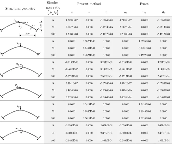
5.3 A Two-End Hinged Beam

After examination of the displacement's quality, it is better to verify the internal forces, since the suggested element is formulated based on the equilibrium equations. For this purpose, the beam with mechanical and geometrical properties similar to the previous test is utilized. Figure 3 shows this structure with R₀ =25andR₀ t =100. An external bending moment of m_z = 2 is applied at

Figure 3: A two-end hinged parabolic beam with a discontinuity in bending moment.

Figures 4, 5 and 6 illustrate the internal forces versus horizontal distance from center line. These distances are found from equationH = R .tan₀ j. Based on the potential energy principles, all

internal forces are found from below equations.

0 z

0

0.5 ( 1 0.05 . tan ),0 20 M

0.5 (1 0.05 . tan ),-20 0

z

z

m R H

m R H

j j

ì - + £ £

ïï

= í_{ï + £ £}

ïî (24)

x

N =0.5m_z.( 0.05 sin )- j ₍₂₅₎

=

-Vy 0.5m_z.( 0.05 cos )j ₍₂₆₎

Figure 5: Distribution of axial force in the two-end hinged parabolic beam.

Figure 6: Distribution of shear force in the two-end hinged parabolic beam.

5.4 Cantilever Parabolic Beam

Figure 7 shows a cantilever parabolic beam, with

R

0



25

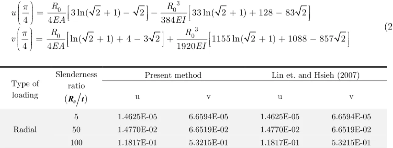
, which is tested in this section. Mechani-cal properties of this structure are similar to the structure in section 5.2. Radial and tangential dis-placements of this beam are obtained for the radial concentrated unit load at the free-end. Tangent angle of the beam’s end is equal to α =45°. Table 3 illustrates all displacements of this structure versus the slenderness ratio. The answers are compared with the obtained results, for the composite curved beams Lin and Hsieh (2007). By assuming the equal transverse and longitudinal modulus, the anisotropic material reduces to an isotropic one, and in this case, the answers are comparable. For this cantilever parabolic beam, tangential and radial displacements are calculated from equation (27).

Figure 7: Geometry of a cantilever parabolic beam Lin and Hsieh (2007) .

3

0 0

3

0 0

3 ln( 2 1) 2 33 ln( 2 1) 128 83 2

4 4 384

ln( 2 1) 4 3 2 1155 ln( 2 1) 1088 857 2

4 4 1920

R R

u

EA EI

R R

v

EA EI

p

p

æ ö÷ é ù é ù

ç ÷ = + - - + +

-ç ÷ ê ú ê ú

ç ÷ ë û ë û

è ø

æ ö÷ é ù é ù

ç ÷ = + + - + + +

-ç ÷ ê ú ê ú

ç ÷ ë û ë û

è ø

(27)

Lin et. and Hsieh (2007) Present method

Slenderness ratio

0

R t

( )

Type of

loading u v u v

6.6594E-05 1.4625E-05

6.6594E-05 1.4625E-05

5

Radial 50 1.4770E-02 6.6519E-02 1.4770E-02 6.6519E-02

5.3215E-01 1.1817E-01

5.3215E-01 1.1817E-01

100

Table 3: Load point displacements in cantilever parabolic beam.

5.5 Parabolic Beam in Pure Bending

The geometry of a parabolic beam, with R0 =25 and a couple of moments at two ends, is shown

tioR₀ t =100, the radial displacement is achieved for variable α. Table 4 demonstrates the results

of proposed method, along with the one obtained by Lin and Hsieh (2007).

Figure 8: A parabolic beam under pure bending Lin and Hsieh (2007).

2

0 1 1 5 2 1 4 1 2

( ) cos tan tan sin .(9 4 tan ) ln(sec tan )

3 3 48 8 16

R v

EI

j = é_êê- + j+ j+ j+ j + j j+ j ùú_ú

ë û (28)

20 30

40 50

60 70

80

α -Degree

3.1309E-03 8.2895E-03

1.9176E-02 4.5322E-02

1.2653E-01 5.3415E-01

6.9955E+00 Present method

answers

3.1309E-03 8.2895E-03

1.9176E-02 4.5322E-02

1.2653E-01 5.3415E-01

6.9955E+00 Lin and Hsieh

(2007)

Table 4: Radial displacement at the middle point of a parabolic beam in pure bending.

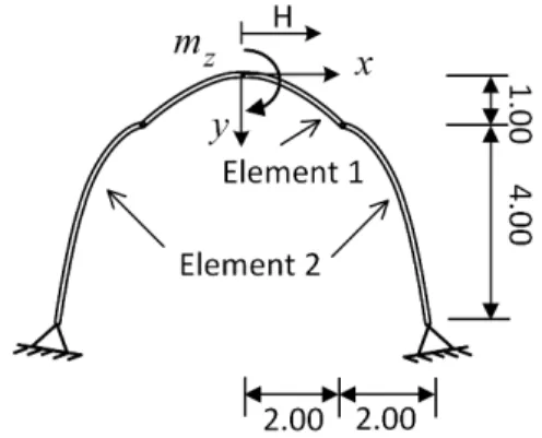
5.6 Arch Structure

A structure which is formed by three parabolic arches, with different geometries, is shown in Figure 9. This arch is modeled with three elements. Element 1 with (R0)1 =2 and t =0.01 is assembled with two half-arches of element 2, having (R0)2 =0.5 andt =0.0025. In fact, the slenderness ratios (R₀ t =200) for both elements are the same. The parabolic vertex is carrying a moment of

z

m = 2. All of mechanical properties are considered to be similar to the one in section 5.2. Table 5

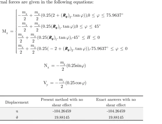
gives the middle-point displacements. Figures 10, 11 and 12 illustrate internal forces versus horizon-tal distance from the center line. These distances are calculated by employing equation (29).

0.5tan 2 , -4 -2; -75.9637 0

H 2 tan , -2 2; -45 45

0.5tan 2 , 2 4;0 75.9637 H

H H

j j

j j

j j

ìï - £ £ £ £

ïï ïï

=_íï £ £ £ £

ïï + £ £ £ £

ïïî



 



(29)

Exact internal forces are given in the following equations:

0

0

0

0

R

R

R

R

z z

2

z z

1 z

z z

1

z z

2

(0.25(2 ( ) . tan )),0 75.9637

2 2

(0.25( ) . tan ),0 45

2 2

M

(0.25( ) . tan ),-45 0

2 2

(0.25( 2 ( ) . tan )),-75.9637 0

2 2

m m

m m

m m

H

m m

j j

j j

j

j j

ìïï- + + £ £

ïï ïï

ïï- + £ £

ïïï = í

ïï _{+ £ £}

ïï ïï

ïï _{+ - + £ £}

ïïïî









(30)

z x

N (0.25sin )

2

m

j

= - (31)

y

V (0.25 cos )

2

z m

j

= - (32)

Exact answers with no shear effect Present method with no

shear effect Displacement

-104.26459 -104.26459

u

19.88145 19.88145

θ

Figure 11: Distribution of the axial force in arch structure.

Figure 12: Distribution of the shear force in arch structure.

5.7 Sinusoidal Loading

case and the second one are pinned-pinned and pinned-roller, respectively. Two pinned supports make the beam statically indeterminate, but a pinned-roller beam is a determinate structure. A sinusoidal distributed load is applied to the beam with a maximum amount of a unit at the middle point. It should be noted, the geometry, cross section properties and mechanical characteristics are similar to the upper part of the structure shown in Figure 9. In this solution, only the bending ef-fect is taken into account, due to negligibility of the axial and shear efef-fects. Obtained results of the displacements with different meshes are shown in Table 6. By utilizing only one element, the an-swers for this complex loading are precise with zero errors. This is the result of using the exact solu-tion and also satisfying the equilibrium equasolu-tions.

(1) (2)

Figure 13: Parabolic structures with sinusoidal load.

Displacements of node-3 in Fig. 13-2 Displacements of node-2 in Fig. 13-1

θ

v

θ

v u

-0.6354 -1.0707

0.0000 0.0180

0.0000 Exact

-0.6354 -1.0707

ــــــــ ــــــــ

ــــــــ 1-element

Present Method

-0.6354 -1.0707

0.0000 0.0180

0.0000 2-element

-0.6354 -1.0707

ــــــــ ــــــــ

ــــــــ 3-element

ــــــــ ــــــــ

0.0000 0.0180

0.0000 4-element

Table 6: Displacements of the beam with distributed load.

6 CONCLUSION

con-be utilized in the analysis of any parabolic structure. Utilizing suggested explicit form of the con-beam stiffness matrix, which is available in appendix, can accelerate the analysis procedure considerably.

References

Ashwell, D. G. and Sabir, A. B., (1971), Limitations of certain curved finite elements when applied to arches,Int. J. mech. Sci. 13:133-139.

Babu, C. R. and Prathap, G., (1995), A linear thick curved beam element, Int. J. Numer. Meth. Engng. 55:379–386. Benedetti, A. and Tralli, A., (1989), A new hybrid f.e. model for arbitrarily curved beam-i. linear analysis, Comput. Struct. 33(6):1437-1449.

Chapelle, D., (1997), A locking-free approximation of curved rods by straight beam elements, Numer. Math. 77: 299– 322.

Choi, J. K. and Lim, J. K., (1993), Simple curved shear beam elements, Commun. Numer. Meth. Engng. 9:659-669. Choi, J. k. and Lim, J. k., (1995), General curved beam elements based on the assumed strain fields, Comput. Struct. 55(3):379-386.

Dawe, D. J., (1974), Curved finite elements for the analysis of shallow and deep arches, Comput. Struct. 4:559-580. Gimena, L., Gonzagay, P. and Gimena, F., (2010), Forces, moments, rotations, and displacements of polynomial-shaped curved beams, Int. J. Struct. Stab. Dyn. 10(1):77-89.

Gutierrez, R. H., Laura, P. A. A., Rossi, R. E., Bertero, R. and Villaggi, A., (1989), In-plane vibrations of non-circular arcs ofnon-uniform cross-section, J. Sound. Vibr. 129(2):181-200.

Huang, C. S., Tseng, Y. P. and Chang, S. H., (1998), Out-of-plane dynamic responses of non-circular curved beams by numerical Laplace transform, J. Sound Vibr. 215(3):407-427.

Huang, C. S., Tseng, Y. P., Leissa, A. W. and Nieh, K. Y., (1998), An exact solution for in-plane vibrations of an arch having variable curvature and cross section, Int. J. Mech. Sci. 40(11):1159–1173.

Kikuchi, F. and Tanizawa, K., (1984), Accuracy and locking-free property of the beam element approximation for arch problems, Comput. Struct. 19:103–110.

Kikuchi, F., (1975), On the validity of the finite element analysis of circular arches represented by an assemblage of beam elements, Comput. Methods Appl. Mech. Engng. 5:253–276.

Kim, J. G. and Kim, Y. Y., (1998), A new higher-order hybrid-mixed curved beam element, Int. J. Numer. Meth. Engng. 43:925-940.

Kim, J. G. and Lee, J. K., (2008), Free-vibration analysis of arches based on the hybrid-mixed formulation with consistent quadratic stress functions, Comput. Struct. 86:1672–1681.

Kim, J. G. and Park, Y. K., (2008), The effect of additional equilibrium stress functions on the three-node hybrid-mixed curved beam element, J. Mech. Sci. Tech. 22:2030-2037.

Lee, B. K. and Wilson, J. F., (1989), Free vibrations of arches with variable curvature, J. Sound Vibr. 136:75–89. Lee, B. K., Oh, S. J., Mo, J. M. and Lee, T. E., (2008), Out-of-plane free vibrations of curved beams with variable curvature, J. Sound Vibr. 318:227–246.

Lee, P. G. and Sin, H. C., (1994), Locking-free curved beam element based on curvature, Int. J. Numer. Meth. Engng. 37:989-1007.

Lin, K. C. and Hsieh, C. M., (2007), The closed form general solutions of 2-d curved laminated beams of variable curvatures, Compos. Struct. 79:606-618.

Lin, K. Ch. and Huang, Sh. H., (2007), Static closed-form solutions for in-plane thick curved beams with variable curvatures, J. Sol. Mech. Mater. Engng. 1(8).

Marquis, J. P. and Wang, T. M., (1989), Stiffness matrix of parabolic beam element, Comput. Struct. 31(6):863–870. Meck, H. R., (1980), An accurate polynomial displacement function for finite ring elements, Comput. Struct. 11:265-269.

Molari, L. and Ubertini, F., (2006), A flexibility- based finite element for linear analysis of arbitrarily curved arches, Int. J. Numer. Methods Engng. 65:1333–1353.

Oh, S. J., Lee, B. K. and Lee, I. W., (1999), Natural frequencies of noncircular arches with rotary inertia and shear deformation, J. Sound Vibr. 219(1):23–33.

Oh, S. J., Leeb, B. K. and Lee, I. W., (2000), Free vibrations of non-circular arches with non-uniform cross-section, Int. J. Solids Struct. 37:4871-4891.

Pandian, N., Appa Rao, T. V. S. R., and Chandra, S., (1989), Studies on performance of curved beam finite elements for analysis of thin arches, Comput. Struct. 31(6):997-1002.

Prathap, G. and Naganarayana, B. P., (1990), Analysis of locking and stress oscillations in a general curved beam element, Int. J. Numer. Meth. Engng. 30:177–200.

Raveendranath, P., Singh, G. and Pradhan, B., (1999), A two-noded locking-free shear flexible curved beam ele-ment”, Int. J. Numer. Meth. Engng. 44:265-280.

Raveendranath, P., Singh, G. and Rao, G.V., (2001), A three-noded shear flexible curved beam element based on coupled displacement field interpolations, Int. J. Numer. Meth. Engng. 51:85–101.

Sabir, A. B. and Ashwell, D. G., (1971), A comparison of curved beam finite elements when used in vibration prob-lems,J. Sound. Vibr. 18(4):555-563.

Shahba, A., Attarnejad, R., Jandaghi Semnani, S. and Honarvar Gheitanbaf, H., (2013), New shape functions for non-uniform curved timoshenko beams with arbitrarily varying curvature using basic displacement functions, Mec-canica, 48:159–174.

Stolarski, H. and Belytschko, T., (1982), Membrane locking and reduced integration for curved beams, J. Appl. Mech. 49:172–176.

Tarnopolskaya, T., Hoog, F. D., Fletcher, N. H. and Thwaites, S., (1996), Asymptotic analysis of the free in-plane vibrations of beams with arbitrarily varying curvature and cross-section, J. Sound Vibr. 196(5):548-579.

Yang, S.Y. and Sin, H. C., (1995), Curvature-based beam elements for the analysis of timoshenko and shear-deformable curved beams, J. Sound. Vibr. 18:7569–84.

APPENDIX - EXPLICIT FORM OF THE PARABOLIC BEAM STIFFNESS MATRIX

11 2,3 5,5 5,3 6,3 5,4 4,6 5,6 2,3 4,5 4,3 6,3 4,4 3,2 6,2 2,3 5,5 5,2 6,3 6,2 5,3 4,6 5,6 6,2 2,3 4,5 4,2 6,3 6,2 4,3

12 1,4 5,6 5,4 4,5 5,5 1,4 4,6 4,4 3,2

1

((( ) ( )) (

) ( ))

1

(((( ) ( ))

G m m m m m m m m m m m m m m m

D

m m m m m m m m m m m m m m

G m m m m m m m m m

D

= - + - - + +

-- + + +

-= - - - - _{1,2 5,6 5,2 4,5 5,5}

1,2 4,6 4,2 6,3 3,2 6,2 4,3 5,5 5,3 4,5

13 4,5 5,6 5,5 4,6 1,4 4,4 5,5 5,4 4,5 6,2 4,5 5,6 5,5 4,6 1,2 4,2 5,5 5,2 4,5 2,3 4,3 5,6 5,3

( )

( )) ( )( ))

1

(((( ) ) ( )

) ((

m m m m m

m m m m m m m m m m

G m m m m m m m m m m m m m m m

D

m m m m m m m m m

+ - + +

- - - + - +

= - + - + +

-+ - + - _{4,6 1,4 4,3 5,4 5,3 4,4 6,2 6,3 5,4}

5,3 4,6 5,6 4,3 6,3 4,4 1,2 6,3 4,2 5,6 4,6 5,2 1,4 5,2 4,4 4,2 5,4 6,3 4,2 5,3 5,2 4,3

) ) ((

) ( )) ( ) ( )

)

m m m m m m m m

m m m m m m m m m m m m m m m m m

m m m m m

- + +

-+ + - + - - + - +

15 1,4 4,6 4,4 6,3 4,3 2,3 4,5 3,2 1,2 4,6 4,2 6,3 6,2 2,3 4,5 4,3

16 4,5 5,6 5,5 4,6 1,4 4,4 5,5 5,4 4,5 3,2 4,5 5,6 5,5 4,6 1,2 4,2 5,5 5,2 4,5 2,3 4,3

1 ((( ) ) ( ) ( )) 1 (((( ) ) ( ) ) ((

G m m m m m m m m m m m m m m m

D m

G m m m m m m m m m m m m m m m

D

m m m m m m

= - - + - + + -

-= - - + - + +

-+ - + _{5,6 5,3 4,6 1,4 4,3 5,4 5,3 4,4 3,2 4,3 5,6}

5,3 4,6 1,2 4,2 5,3 5,2 4,3

21 2,1 6,3 6,1 2,3 5,6 6,1 2,3 5,5 5,3 6,3 2,1 5,5 5,1 4,5 5,6 6,1 4,3 4,1 6,3

22 6,3 ) ) ( ) ) 1 ((( ) ( ) ( )) ( )) 1 (

m m m m m m m m m m m

m m m m m m m

G m m m m m m m m m m m m m m

D

m m m m m

G m D - - + + -+ - + = - - + + - + + --

-= _{4,1 5,5 5,1 4,5 6,1 4,3 5,5 5,3 4,5}

23 5,6 5,5 2,3 5,3 6,1 6,3 5,6 5,5 2,1 5,1 1,4 2,1 5,3 2,1 6,3 5,4 5,1 2,3 6,1 2,3 5,4 4,5 5,6 6,1 4,3 4,1 6,3 1,4 2,3

( ) ( ))

1

((((( ) ) (( ) ))

) ( ) (

m m m m m m m m m

G m m m m m m m m m m m m m

D

m m m m m m m m m m m m m m m m m

- + +

-= - - + - - - + - +

- - + + - + - _{4,4 5,5}

4,3 5,4 5,3 4,4 6,1 4,1 5,4 5,5 4,4 2,1 5,1 4,4 6,3 2,1 4,3 5,5 4,1 5,3 4,1 2,3 5,5 5,1 4,3

24 6,1 2,3 5,5 5,3 6,3 2,1 5,5 5,1 25 6,1 2,3 4,5 4,3 6,3 2,1 4

) ( ) ) 1 ( ( ) ( )) 1 ( ( ) ( m

m m m m m m m m m m m m m m m m m m

m m m m m

G m m m m m m m m

D

G m m m m m m m

D

- + + + - -

-+ +

= - + +

-= - - + + _{,5 4,1}

26 2,3 4,1 2,1 4,3 5,5 4,1 5,3 2,1 5,3 4,5 5,1 2,3 4,5 5,1 4,3

))

1

(( ) )

m

G m m m m m m m m m m m m m m m

D

-= - - + - +

31 2,1 5,5 5,1 6,1 5,4 4,6 5,6 2,1 4,5 4,1 6,1 4,4 3,2 2,1 6,2 5,5 5,1 6,2 6,1 5,2 4,6 5,6 4,1 6,2 2,1 6,2 4,5 6,1 4,2

32 1,4 5,6 5,4 4,5 5,5 1,4 4,6 4,4 3

1

((( ) ( )) (

) ( ))

1

(((( ) ( ))

G m m m m m m m m m m m m m m m m

D

m m m m m m m m m m m m m

G m m m m m m m m m

D

= - + - + - + +

- + - - + +

= - - + + - _{,2 1,2 5,6 5,2 4,5 5,5}

1,2 4,6 4,2 6,1 3,2 6,2 4,1 5,5 5,1 4,5

33 1,4 4,5 5,6 5,5 4,6 4,4 5,5 5,4 4,5 6,2 4,5 5,6 5,5 4,6 1,2 4,2 5,5 5,2 4,5 2,1 5,1 4,6 4,1

( )

( )) ( )( ))

1

((( ( ) ) ( )

) ((

m m m m m

m m m m m m m m m m

G m m m m m m m m m m m m m m m

D

m m m m m m m m m

+ -

-- - - +

-= - + - + - +

- + + - _{5,6 1,4 5,1 4,4 4,1 5,4 6,2 6,1 5,4}

5,1 4,6 5,6 4,1 6,1 4,4 1,2 6,1 5,6 4,2 5,2 4,6 1,4 4,2 5,4 5,2 4,4 6,1 5,1 4,2 4,1 5,2

34 1,4 5,6 5,4 6,1 2,1 5,5 5,1 3,2

) ) ((

) ( )) ( ) ( )

) -1

((( ) ) (

m m m m m m m m

m m m m m m m m m m m m m m m m m

m m m m m

G m m m m m m m m

D

- + +

- - - + - - + + - +

+

-= - - + + _{1,2 5,6 5,2 6,1 6,2 2,1 5,5}

5,1

35 1,4 4,6 4,4 6,1 2,1 4,5 4,1 3,2 1,2 4,6 4,2 6,1 6,2 2,1 4,5 4,1

36 3,2 4,1 1,2 4,5 5,4 4,4 2,1 5,5 5,1 4,2 5,1 5,2 4,1

) ( )) 1 ((( ) ) ( ) ( )) 1 ( (( ) ( ))

m m m m m m m

m

G m m m m m m m m m m m m m m m

D m

G m m m m m m m m m m m m m

D

- + +

-= - - + + - + +

-= - - + - - + + _{2,1 5,2 4,5}

4,2 5,5 1,2 3,2 1,4 2,1 4,5 4,1 5,6 4,6 2,1 5,5 5,1

(

) ( )(( ) ( )))

m m m

m m m m m m m m m m m m m

-1,4 5,6 5,4 4,5 5,5 1,4 4,6 4,4 2,3 4,3 5,6 5,3 4,6 1,4 5,3 4,4 4,3 5,4 6,1 1,4 5,6 5,4 4,5 5,5 1,4 4,6 4,4 2,1 4,1 5,6 5,1 4,6 1,4 4,4 5,1 4,1 5,4 6,3 4,3 5,

((( ) ( )) ( )

) ((( ) ( )) ( )

) (

D m m m m m m m m m m m m m m m m

m m m m m m m m m m m m m m m m m

m m m m m m m

= - - - + - +

-+ + - + + - +

-+ - + _{5 5,3 4,5 2,1 4,1 5,5 5,1 4,5 2,3 5,1 4,3}

4,1 5,3 3,2 1,2 5,6 5,2 4,5 5,5 1,2 4,6 4,2 2,3 5,3 4,6 4,3 5,6 1,2 4,2 5,3 5,2 4,3 6,1 1,2 5,6 5,2 4,5 5,5 1,2 4,6 4,2

) ( )

) ((( ) ( )) ( )

) ((( ) (

m m m m m m m m m m

m m m m m m m m m m m m m m m m m

m m m m m m m m m m m m m

- + - +

-+ + - + + - + - +

+ - + - - - _{2,1 5,1 4,6}

4,1 5,6 1,2 4,1 5,2 4,2 5,1 6,3 4,3 5,5 5,3 4,5 2,1 4,1 5,5 5,1 4,5 2,3 5,1 4,3 4,1 5,3 6,2

3

2 2 0 1 1 0 1 1 0 2 2 0 0

1 2 3 1 1

)) (

) ) (( ) ( )

)

( ) ( ) ( )(

4

i j i j i j i j

ij i

m m m

m m m m m m m m m m m m m m m m m m

m m m m m

G G R G G R G G R G G R R

S I I I G G

EA kGA EA kGA EI

+

- + - - - + - +

- +

= + + + + 0 0

4

3 2

0 1 2 2 1 0 1 3 3 1 0

1 2 2 1 5 6 7 3 3

2 3

0 2 3 3 2 0

8 2 2 9

3

1 ₂ 2 3

) ( )

( ) ( )

( ) . . ( )( )

2 2

( )

( )( ) . , , 1, 2, 3

sin ( ) 1 sin(

0.5.( sin( ) ), , (

6 cos ( )

j

i j i j i j i j

i j i j i j

i j i j

i j

R R

I

kGA EA

R G G G G R G G G G R

G G G G I I I G G

EI EI EI

R G G G G

R

I G G I i j

EI EI

I a a L I L I

a + -+ + + + + + - + + + = = + - = =

6 4 2

4 5 6 _{4 2}

3 3

7 ₂ 8 _{2 2}

) 5 sin( ) 5 sin( ) 5 ),

24 16 16

cos ( ) cos ( ) cos ( ) sin( ) sin( )

1 1 3 3

( 1), 0.2.( 1), 0.25.( ),

cos( ) cos( ) cos ( ) 2cos ( ) 2

sin( ) sin ( ) 1sin ( ) 1

0.2.( ), 0.25.( sin(

2 2

cos ( ) cos ( ) cos ( )

L

I I I L

I L I

a a a

a a a

a a

a a a a

a a a

a a a

+ +

-= - = - = + +

= + = + + ₉

, 0 3,

1 1 1

) ), .( 1)

2 3 cos( )

ln(sec( ) tan( ))

( , ) , ( , ) , 1, 2, 3, 1, 2, 3, 4, 5, 6

i j q i j q

L I

L

m N i j _j m N i j _{j a} i j

a a a a = + = - = -= + = = = =