Synchronization Control of Uncertain Generalized Lorenz Chaotic System: Chattering-Free Sliding Model Control

(1)



Abstract—In this paper, we propose a chattering-free sliding mode control (SMC) scheme for the synchronization of generalized Lorenz chaotic systems with unmatched uncertainties. The concept of quasi sliding mode controller (QSMC) is newly introduced to avoid chattering phenomenon that frequently appears in the conventional sliding mode control systems. The error states between drive and response systems can be stabilized and driven into an arbitrary and predictable neighborhood of zero even with unmatched uncertainties. An example is given to illustrate the effectiveness of the proposed chattering-free SMC developed in this paper.

Index Terms—Sliding mode control; Chattering-free; Synchronization; Chaos; Generalized Lorenz chaotic system

I. INTRODUCTION

esigning a system to mimic the behavior of another chaotic system is called synchronization. The two chaotic systems are generally called drive (master) and response (slave) systems, respectively. Chaos synchronization can be applied in the wide fields of physics and engineering systems such as power converters, chemical reactions, biological systems, information processing, and especially for secure communication. Up to now, many control methods such as adaptive control [2,9], sliding mode control [3,13], fuzzy control [6,8,12], backstepping control [11,14] have been employed to synchronize chaotic systems with different initial conditions. However, in the conventional SMC systems [1,3,13], ideal sliding mode only exists for infinite frequency switching operation. From practical point of view, thus control input is impossible to implement and will cause the undesired chattering phenomenon [4]. Consequently, there are a lot of control methods in the literature to suppress the chattering phenomenon. For instance, in [5], authors used the concept of ‘extended system’ by introducing a new state such that the control input becomes continuous as a result of integral function. However, the major problem in this method is that the external disturbance should be enlarged and the control signal might become saturated. In the methods of [6,8], fuzzy control is utilized to effectively eliminate the chattering. But these methods proposed above should increase the complexity of control circuits and the cost for implementing such control circuit might be increase. In [10], the control

a_{The authors are with the Department of Computer and Communication,}

Shu-Te University, Kaohsiung 824, Taiwan.

b _{The author is with the Department of Engineering Science, National Cheng}

Kung University, Tainan 701, Taiwan.

* Corresponding author: J. J. Yan (E-mail: jjyan@ stu.edu.tw).

input is switched to reduce the chattering when the system trajectories enter a specified layer close to the switching surface. However, the relations between the layer bound and steady error are still necessary to be further discussed. Furthermore, most of controllers in above papers are carried out with an ideal assumption of matched uncertainties. The error bound of synchronization, due to the mismatch uncertainties, is not well discussed and cannot be predicted or estimated in their work.

II. SYSTEM DESCRIPTION AND PROBLEM FORMULATION

In this section, we consider the robust synchronization of two identical GLCSs.

A. Generalized Lorenz chaotic systems We consider the following GLCS:





T





T

x x x x

x x

t x t x t x k t

x

t x t x t x k t x k t

x

t x t x k t

x

30 20 10 3

2 1

2 1 3 3

3 1 2 1

2

1 2 1

) 0 ( ) 0 ( ) 0 (

) ( ) ( ) ( ) 87

1 3 8 ( ) (

) ( ) ( ) ( ) 1 ( ) ( ) 29 35 28 ( ) (

)] ( ) ( [ ) 29 25 10 ( ) (

  

 

 

 



   

  

(1)

where





3

3 2

1() () ()

)

(t x t x t x t R

x  T is the state vector,





T

x x

x10 20 30 is the initial value vector, and k is the

system parameter with0k1. Obviously, the original Lorenz system is a special case of system (1) with k0.3

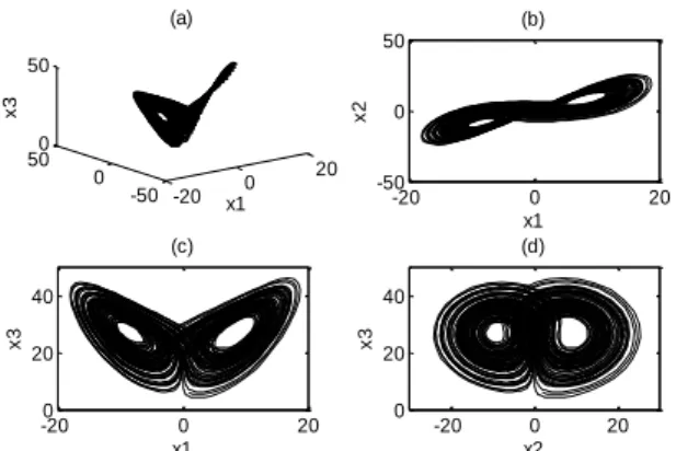
The dynamics of this system has been extensively studied in [16] for a space range of the amplitude of the term k and displays chaotic behavior for each0k1. Fig. 1 (a)-(d) show the chaotic motion of system (1) for k0.3 with initial condition of





T





T

x x

x10 20 30  1 2 6 . In the

following, we will consider the synchronization of two

Synchronization Control of Uncertain

Generalized Lorenz Chaotic System:

Chattering

-

Free Sliding Model Control

Sheng-Wen Chen

a

_{, Yi-Sung Yang}

b

_{, Pei-Zhi Zhang-Jian}

a

_{, Teh-Lu Liao}

b

, Jun-Juh Yan

a

*

D

The purpose of this paper lies in the development of a chattering-free QSMC for synchronizing the state trajectories of two GLCSs. A new concept of QSMC is introduced such that continuous control input is obtained to avoid chattering phenomenon. A switching surface only including partial states is adopted to ensure the bounds of the error dynamics in the quasi sliding manifold. Then a QSMC is derived to guarantee the occurrence of the quasi sliding manifold and the error states between drive and response systems can be stabilized and driven into an arbitrary and predictable neighborhood of zero even with unmatched uncertainties.

Proceedings of the International MultiConference of Engineers and Computer Scientists 2013 Vol I, IMECS 2013, March 13 - 15, 2013, Hong Kong

ISBN: 978-988-19251-8-3

ISSN: 2078-0958 (Print); ISSN: 2078-0966 (Online)

(2)

GLCSs and give an explicit and simple procedure to establish a QSMC to achieve the control goal.

B. Synchronization problem formulation

Consider the following two GLCSs, where the drive system and response system are denoted with x and y, respectively. Drive system: ) ( ) ( ) ( ) 87 1 3 8 ( ) ( ) ( ) ( ) ( ) 1 ( ) ( ) 29 35 28 ( ) ( )] ( ) ( [ ) 29 25 10 ( ) ( 2 1 3 3 3 1 2 1 2 1 2 1 t x t x t x k t x t x t x t x k t x k t x t x t x k t x                 (2) Response system: ) ( ) ( ) ( ) ( ) 87 1 3 8 ( ) ( ) ( ) ( ) ( ) ( ) ( ) 1 ( ) ( ) 29 35 28 ( ) ( ) ( )] ( ) ( [ ) 29 25 10 ( ) ( 3 2 1 3 3 2 3 1 2 1 2 1 1 2 1 t d t y t y t y k t y t u t d t y t y t y k t y k t y t d t y t y k t y                     (3)

In general, the unmatched uncertainties d_i(t),i1,2,3 are assumed bounded, respectively, by

3 , 2 , 1 , )

(t  i

d_i _i (4) where



i



0

are given.

We introduce the single control input u into the second equation in response system (3). Let us define the synchronization errors between the response system (3) and the drive system (2) as follows:









T

T t x t y t x t y t x t y t e t e t e t E ) ( ) ( ) ( ) ( ) ( ) ( ) ( ) ( ) ( ) ( 3 3 2 2 1 1 3 2 1    

 ₍₅₎

, then the dynamics of the error system is determined, as follows: ) ( ) ( ) ( ) ( ) ( ) ( ) 87 1 3 8 ( ) ( ) ( ) ( ) ( ) ( ) ( ) ( ) ( ) 1 ( ) ( ) 29 35 28 ( ) ( ) ( )] ( ) ( [ ) 29 25 10 ( ) ( 3 2 1 2 1 3 3 2 3 1 3 1 2 1 2 1 1 2 1 t d t x t x t y t y t e k t e t u t d t x t x t y t y t e k t e k t e t d t e t e k t e                       (6)

The objective of this study is stated as follows: giving the drive system as (2), the chattering-free QSMC will be designed in spite of the unmatched uncertainties so that the resulting synchronization error can be driven to predictable bounds, i.e. 3 , 2 , 1 ,

lim  



 ei i i

t 

(7) where _i 0 are constants, which are dependent on unmatched uncertainties and the parameter chosen in the QSMC specified later.

III. DEFINITION OF QUASI SLIDING MANIFOLD AND SWITCHING SURFACE DESIGN OF SYNCHRONIZATION

Synchronizing the GLCSs as (2) and (3) by using the QSMC technique involves two major phases. First, an appropriate switching function for the system must be selected such that the error dynamics in quasi sliding manifold can result inlim  , 1,2,3.



 ei i i

t 

Second, a QSMC scheme must be designed to guarantee the existence of quasi

sliding manifold. To complete the above two phases, a switching function is defined as follows:

) ( ) ( )

(t e₂ t e₁ t

s   (8) where sR and



1 is a designed constant. Before continuing our discussion, we first give the definition of quasi sliding manifold as follows.

Definition 3.1: The error system is said to be in the quasi

sliding manifold if there exist _Q0 and t_Q0 such that any solution x() of the error system (6) satisfies

Q t s() , for all

Q t t .

Obviously if the controlled system is in the quasi sliding manifold, from (6), (8) and Definition 3.1, the following dynamics of e1(t) can be obtained as

) ( ) ( ) 29 25 10 ( ) ( ) ( )] ( ) ( ) ( [ ) 29 25 10 ( ) ( 1 1 1 1 1 1 1 t d t s k t e t d t e t e t s k t e               (9)

where ₎₍₁ ₎

29 25 10 (

1 

   k 

Solving the differential equation (9) for e₁(t) when Q t t results in



  

   t  

t t Q t t Q

Q _e _t _e _k _s _d _d

e t

e ( ) ₁

1 ) (

1 ) ( ) ( )]

29 25 10 [( ) ( )

( 1 1     (10)

Since the system is in the quasi sliding manifold,

Q t s() and the bound of e₁(t) can be estimated by

1 ) ( 1 1 ) ( 1 ) ( 1 ) ( 1 1 1 1 1 1 ] ) 29 25 10 [( ) ( )] ( ) ( ) 29 25 10 [( ) ( ) (            Q Q Q Q t t Q Q t t t t t Q t t e k t e e d d s k e t e e t e                 

_

(11)

Furthermore, since



1 is determined such that 0 ) 1 )( 29 25 10 (

1   

 k , the bound for e₁(t) is obtained as 1 1 1 1 1 1 1 / ] ) 29 25 10 [( ) ( lim                  Q Q

t e t k

(12) Furthermore, by (8), the bound for e₂(t)when the time

 

t can be also obtained as

1 2 1 1 2 ) ( lim ) ( lim ) ( ) ( lim ) ( lim











               Q t t t t t e t s t e t s t e (13) Since both e₁(t) and e₂(t) converge to

1  and

2  , respectively, as discussed above, there always exists a time point t such that_ e_i _i, i1,2, fortt_. Thus solving the differential eqn. (6) for state e₃(t) when tt_ results in

          d d x x y y e t e e t e t t t k t t k )] ( ) ( ) ( ) ( ) ( [ ) ( ) ( 3 2 1 2 1 ) ( ) 87 1 3 8 ( 3 ) ( ) 87 1 3 8 ( 3    



      (14)

Furthermore, according to Theorem 1 in [15], the state response of GLCS (2) is contained in the sphere  given by

      _ _ _ _ _ 

 2 2

3 2 2 2 1 3 2 1 ) 29 10 38 ( ] , ,

[x x x x x x k R

, where

ISBN: 978-988-19251-8-3

(3)

) 1 )( 29 264 15 (

) 29 8 ( ) 29 5 19

( 2 2

2

k k

R

 

 

 (15)

, thus the bound for e₃(t)with t can be also obtained as

) 87

1 3 8 (

] )

( [ )

(

lim 1 2 1 2 3

3 3

k R

t e t



   

  

     

(16) Obviously, by (12), (13) and (16), it reveals that the bounds of _i,i1,2,3 are relative to

Q

 . Therefore, to control the system with a smaller value of

Q

 is important and the solution is given in the following section.

IV. QSMC DESIGN FOR QUASI SLIDING MANIFOLD

To ensure the occurrence of the quasi sliding manifold, the continuous QSMC is proposed as

 

  

s s w t

u )( (17)

, where

2 1 3 1 3 1 2

1

)] 29 25 10 (

) 1 [( )] 29 25 10 ( ) 29 35 28 [(

  

 

    



  

  

x x y y e k

k e k k

,

1 

w

and





0 .

The proposed control scheme above will guarantee the occurrence of quasi sliding manifold for the system (6), and is proven in the following theorem.

Theorem 1: Consider the error system (6), if this system is controlled by u(t) in (17). Then the system trajectory converges to the quasi sliding manifold with

1 )

(

  

w w t

s _Q  .

Proof: Let the Lyapunov function of the system be 2

2 1 s V  , then taking the derivative of V and introducing (6), (8) and (17) one has

) (

) ) )( 29 25 10 (

) ( )

1 ( ) 29 35 28 ((

) (

1 1 2

2 3 1 3 1 2 1

1 2

  



 



   

  



      



  

s s s w s

d e e k

u t d x x y y e k e k s

e e s s s

V   

(18)

Since 

  _ 

s

s _{, we have}

) 1 (

) (

  



 



w w s w

s w s V

 

  



(19)

Since

w



1

has been chosen in the controller (17), (19) implies thatV0, whenever

1 )

(

  

w w t

s Q



 . That is to

say that s will converges to the region of

1 )

(

  

w w t

s _Q  . Thus the proof is achieved completely.

V. A NUMERICAL EXAMPLE

In this section, simulation results are presented to demonstrate and verify the effectiveness of the proposed QSMC scheme. The system parameter is chosen as k0.3

to guarantee the chaos behavior for the drive GLCS (2). The initial states of the drive GLCS (2) are x₁(0)22 ,

15 ) 0 (

2 

x , x₃(0)12and those of the response GLCS (3) are y₁(0)20, y₂(0)13, y₃(0)12 . The unmatched uncertainties are given as

) 5 sin( 1 . 0 ) (

1 t t

d  , d₂(t)0.2sin(2t) and )

6 cos( 1 . 0 ) (

3 t t

d  , respectively. Obviously, we have 1

. 0 )

( ₁

1 t  

d

, d2(t)2 0.2_,d3(t)30.1_.

The QSMC design procedure for synchronizing the drive and response GLCSs can be summarized as follows:

Step1: According to (8), parameter



₁₀ is selected

such that ₎₍₁ ₎ ₀

29 25 10 (

1   

 k and the stable bound

of error dynamics system (6) in the quasi sliding mode is then ensured.

Step2: Consequently, the switching surface

s

(t

)

is constructed as:

) ( ) ( )

(t e2 t e1 t

s   (20) Select the control parameters in (17) as



_₀_.₀₃ and _w_₄ and according to Theorem 1, we have _₀_.₀₄

Q 

Step3: By (12), (13) and (16), we can calculate the

predictable bounds _,_i_₁_,₂_,₃ i

 as

0249 . 0

1 1 

e ;e₂ ₂0.0649;e₃ ₃1.4862 (21)

Step4: Construct the QSMC from (17) as

03 . 0 4 ) (

  

s s t

u



(22) where

2 1 3

1 3 1 2

1

)] 29 25 10 (

) 1 [( )] 29 25 10 ( ) 29 35 28 [(









  

 



  

 



x x y y e k

k e k k

3 . 0 

k ;



1;₁0.1; ₂0.2

The simulation results are shown in Fig. 2-4 under the proposed continuous QSMC(22). Fig. 2 and Fig. 3 show, respectively, the corresponding _s_(t₎ error state responses between the drive and controlled response GLCSs under the proposed QSMC(22). The continuous QSMC(22) is shown in

ISBN: 978-988-19251-8-3

(4)

Fig. 4. From the simulation result, it shows that the trajectory of error dynamics quickly converges to quasi sliding manifold ₍₎_ _₀_.₀₄

Q

t

s



and the synchronization error

also converges to the predicted bounds as calculated in (21). Also the chattering does not appear due to the continuous control input as shown in Fig. 4.

VI. CONCLUSIONS

In this paper, a chatter-free SMC scheme for the robust synchronization of generalized Lorenz chaotic systems is studied. The concept of QSMC has been introduced firstly to avoid chattering phenomenon. As expected, under the proposed control law, the error states can be stabilized and driven into an arbitrary and predictable neighborhood of zero even when the unmatched uncertainties are present. Numerical simulations have verified the effectiveness of the proposed method.

REFERENCES

[1] T. Y. Chiang, M. L. Hung, J. J. Yan, Y. S. Yang, J. F. Chang, Sliding mode control for uncertain unified chaotic systems with input nonlinearity, Chaos Soltions Fractals, 34 (2007) 437-442.

[2] S. Dadras, H. R. Momeni. Adaptive sliding mode control of chaotic dynamical systems with application to synchronization, Mathematics and Computers in Simulation, 80 (2010) 2245-2257.

[3] Y.C. Hung, J.J. Yan, T.L. Liao, Projective synchronization of Chua's chaotic systems with dead-zone in the control input, Mathematics and Computers in Simulation, 77 (2008), 374-382.

[4] H. Lee, Vadim I. Utkin, Chattering suppression methods in sliding mode control systems, Annual Review in Control, 31 (2007) 179-188. [5] J.S. Lin, J.J. Yan, Robust Synchronization of Two Chaotic Nonlinear Gyros via An Adaptive Controller, International Journal of Nonlinear Sciences & Numerical Simulation, 10 (2009) 797-804.

[6] X.W. Liu, S.M. Zhong, T-S fuzzy model-based impulsive control of chaotic systems with exponential decay rate, Phys. Lett, 4 (2007) 260-370.

[7] J. Lü , G. Chen, D. Z. Cheng, S. Celikovsky, Bridge the gap between the Lorenz system and the Chen system, Int J Bifurcat Chaos, 12 (2002) 2917-2926.

[8] M. Roopaei, M.Z. Jahromi, S. Jafari, Adaptive gain fuzzy sliding mode control for the synchronization of nonlinear chaotic gyros, Chaos, 19 (2009) 013125.

[9] M. Roopaei, B. R. Sahraei, T. C. Lin, Adaptive sliding mode control in a novel class of chaotic systems, Communications in Nonlinear Science and Numerical Simulation, 15 (2010) 4158-4170.

[10] J.E. Slotine, W. Li, Applied Nonlinear Control, Prentice-Hall, New Jersey, (1991).

[11] T. Wu, M.S. Chen, Chaos control of the modified Chua’s circuit system. Physica D , 164 (2002) 53-58.

[12] X. Wu, G. Chen, J.P. Cai, Chaos synchronization of the master–slave generalized Lorenz systems via linear state error feedback control, Physica D: Nonlinear Phenomena, Issue 1, 229 (2007) 52-80 [13] J.J. Yan, M.L. Hung, T.Y. Chiang, Y.S. Yang, Robust synchronization

of chaotic systems via adaptive sliding mode control. Physics Letters A , 356 (2006) 220-225.

[14] J. Zhang, C. Li, H. Zhang, J. Yu, Chaos synchronization using single variable feedback based on backstepping method. Chaos Solitons & Fractals, 21 (2004) 1183–1193.

[15] D. Li, J.A. Lu, X. Wu, G. Chen, Estimating the bounds for the Lorenz family of chaotic systems. Chaos Solitons & Fractals, 23 (2005) 529– 534.

[16] J. Lü , G. Chen, D. Z. Cheng, S. Celikovsky, Bridge the gap between the Lorenz system and the Chen system, Int J Bifurcat Chaos, 12 (2002) 2917-2926.

Fig. 1. (a) Trajectories of GLCS (b) Trajectories projected on the x₁-x₂

plane (c) Trajectories projected on the _x₁ -3

x plane (d) Trajectories projected on the

2

x -_x₃ plane.

Fig. 2. The time response of switching functions(t).

Fig. 3. The time responses of error state.

Fig. 4. The time response of the continuous QSMC (22).

-20 0 20

-50 0 50

x1

x2

(b)

-200 0 20

20 40

x1

x3

(c)

-20 0 20

0 20 40

x2

x3

(d)

-20 0

20 -50

0 500 50

x1 (a)

x3

0 1 2 3 4

-0.5 0 0.5 1 1.5 2 2.5 3 3.5 4

s|(t)|

0 1 2 3 4 5 6

-2 0 2

0 1 2 3 4 5 6

-2 0 2

0 1 2 3 4 5 6

-2 0 2

e1

e2

e3

0 1 2 3 4

-100 -50 0 50 100 150 200

ISBN: 978-988-19251-8-3