Accident Analysis and Prevention

Contents lists available atScienceDirect

Accident Analysis and Prevention

journal homepage:www.elsevier.com/locate/aap

Geographically weighted negative binomial regression applied to zonal level

safety performance models

Marcos José Timbó Lima Gomes

, Flávio Cunto

, Alan Ricardo da Silva

a_{Department of Transportation Engineering, Federal University of Ceará, Brazil} b_{Department of Statistics, University of Brasilia, Brazil}

A R T I C L E I N F O

Keywords:

Safety performance models Spatial dependency Local spatial models

Geographically weighted poisson regression Geographically weighted negative binomial regression

A B S T R A C T

Generalized Linear Models (GLM) with negative binomial distribution for errors, have been widely used to estimate safety at the level of transportation planning. The limited ability of this technique to take spatial e_ffects into account can be overcome through the use of local models from spatial regression techniques, such as Geographically Weighted Poisson Regression (GWPR). Although GWPR is a system that deals with spatial de-pendency and heterogeneity and has already been used in some road safety studies at the planning level, it fails to account for the possible overdispersion that can be found in the observations on road-traffic crashes. Two approaches were adopted for the Geographically Weighted Negative Binomial Regression (GWNBR) model to allow discrete data to be modeled in a non-stationary form and to take note of the overdispersion of the data: the first examines the constant overdispersion for all the traffic zones and the second includes the variable for each spatial unit. This research conducts a comparative analysis between non-spatial global crash prediction models and spatial local GWPR and GWNBR at the level of traffic zones in Fortaleza/Brazil. A geographic database of 126 traffic zones was compiled from the available data on exposure, network characteristics, socioeconomic factors and land use. The models were calibrated by using the frequency of injury crashes as a dependent variable and the results showed that GWPR and GWNBR achieved a better performance than GLM for the average residuals and likelihood as well as reducing the spatial autocorrelation of the residuals, and the GWNBR model was more able to capture the spatial heterogeneity of the crash frequency.

1. Introduction

Most of the available methods for transportation planning have sought to follow a procedure in which the road safety dimension is systematically included at all the stages of its strategy (ITE, 2009). However, giving the inherent stochastic nature of road crashes, the complex environment in which they occur and the major factors that lead to them (as well as the spatial dependency observed among the variables), there have not been yet many studies that include this di-mension in the planning process. Consequently this area of research has not attracted the same interest as studies carried out to evaluate other aspects of transport, such as travel time, average delay, vehicle-miles traveled, among others.

Studies aimed at evaluating the safety performance for planning purposes can be carried out at a more operational and tactical level using individual features of the network. In this case, the modeling process seeks to estimate crashes from safety performance models de-veloped for a given set of links and nodes in the network (Lord and Persaud, 2004; Tarko et al., 2008; Song et al., 2015). Another common

approach is based on real units, usually traffic analysis zones (TAZ), and tries to relate a set of aggregated variables often linked to network attributes, socioeconomic and demographic factors to the frequency and severity of crashes aggregated at the TAZ level (strategic level) (Hadayeghi et al., 2010; Huang et al., 2013; Pulugurha et al., 2013; Pirdavani et al., 2014; Xu and Huang, 2015).

Research endeavours aimed at designing strategic safety perfor-mance models were initially concerned with applying traditional ne-gative binomial distribution to a generalized linear structure (Hadayeghi et al., 2003; Lovegrove and Sayed, 2006). While this fra-mework may be well suited to individual entities (links and nodes) it does not capture the spatial dependency that is usually observed when one aggregates data at the TAZ level.

In addition to spatial dependence, crashes are also subject to spatial heterogeneity, which can be defined as“the continuous space-varying structural relationships describing space-related factors that system-atically vary across the region of interest”(Xu et al., 2017). Due to this aspect, the use of an overall fixed relation between the dependent variable and the explanatory variables for the entire study area can

http://dx.doi.org/10.1016/j.aap.2017.06.011

Received 19 February 2017; Received in revised form 7 June 2017; Accepted 16 June 2017

⁎_{Corresponding author.}

E-mail addresses:timbo@det.ufc.br(M.J.T.L. Gomes),flaviocunto@det.ufc(F. Cunto),alansilva@unb.br(A.R. da Silva).

Available online 22 June 2017

0001-4575/ © 2017 Elsevier Ltd. All rights reserved.

affect the adjustments of the estimates of the individual sites, gen-erating instability in the coefficients of the models. The consideration of spatial heterogeneity using local models such as geographically weighted models provides a better platform that allows exploring the different spatial relationships between road crashes and their risk fac-tors.

The spatial dimension has been incorporated into the modeling framework with a series of global and local spatial models including the following: Conditional Auto-regression (CAR) models, Simultaneous Autoregressive (SAR) models, Spatial Error Models (SEM), auto-regressive models with spatial spillover effects, Geographically Weighted Regression (GWR) and Geographically Weighted Poisson Regression models (GWPR) (Erdogan, 2009; Hadayeghi et al., 2010; Pirdavani et al., 2014; Xu and Huang, 2015; Rhee et al., 2016; Cai et al., 2016). Despite the promising results obtained from these techniques, it appears that Geographically Weighted Negative Binomial Regression Models (GWNBR) may make the overall model more useful by allowing it to incorporate the overdispersion that is usually observed in the data and to use the results in the traditional Empirical Bayes method. This paper presents a comparison between the GWPR and GWNBR models which were designed for a set of TAZ in Fortaleza, Brazil.

2. Background

It is generally recognized that, although it is one of the most im-portant dimensions of transport systems, safety is still not well in-tegrated into the framework of its planning strategies. Several studies have concluded that among the main reasons for a more inclusive methodology for safety, is the lack of a comprehensive integrated da-taset for both crashes and other traffic and road attributes linked to crashes and the somewhat limited scope of the available tools needed for conducting an analysis of safety at this level (Chatterjee et al., 2001; Dumbaugh et al., 2004; Tarko, 2006). These factors lead to a greater reliance on a more subjective approach when adopting strategies or making an assessment of safety in different transport scenarios.

The macro-level safety modeling approach usually makes use of a pre-determined spatial aggregation in which the information regarding some of the possible contributing factors is readily available, such as counties, census tracts, wards and TAZ (Aguero-Valverde and Jovanis, 2006; Quddus, 2008; Siddiqui et al., 2012; Lee et al., 2014). The ex-pected crash frequency is estimated for each TAZ according to a set of contributing factors that can be grouped intofive major categories: land use, road network, traffic exposure, socioeconomic factors and demo-graphic attributes (Quddus, 2008; Abdel-Aty et al., 2013; Xu and Huang, 2015; Rhee et al., 2016; Wang et al., 2016).

Hadayeghi et al. (2010) presented a series of crash prediction models for 463 TAZ in Toronto by applying traditional NB generalized regression (global) and GWPR local models. The results suggested that the GWPR models were able, to some extent, to deal with the spatial dependency as well as the spatial heterogeneity that arose from these factors and TAZ. This study was followed by at least two other research projects undertaken in different jurisdictions, Matkan et al. (2011) using TAZ data for Masshad (Iran) andLi et al. (2013)using county level datasets for California. These studies observed a considerable improvement in model prediction for GWPR models, when compared with the global NB models.

When global regression provides estimates with a low degree of accuracy in some areas, it may be more useful to use a local regression model, since they are able to incorporate spatial relations between variables in a specific way for each study area. Among the geo-graphically weighted models that are suited to the road crash phe-nomenon, there are GWGLM, which extends the concept of the GWR in the context of Generalized Linear Models (GLM). It achieves this by allowing the application of local regression models where the in-dependent variable does not need to be a continuous measurement and the error terms do not necessarily follow a normal distribution pattern

(Chen and Yang, 2012).

2.1. Geographically weighted poisson regression–GWPR

One example of GWGLM is GWPR developed by Nakaya et al. (2005), who proposed this technique as a means of comparing the number of deaths in zones with socioeconomic variables. In the parti-cular case of road safety, some studies have already used GWPR to investigate local spatial variations with regard to the number of crashes in certain areas (Hadayeghi et al., 2010; Li et al., 2013; Pirdavani et al., 2014). The proposed GWPR model is defined by Eq.(1):

∑

∼ ⎡

⎣

⎢ ⎛

⎝

⎜ ⎞

⎠ ⎟⎤

⎦ ⎥ yj Poisson tjexp β u v x( , )

k

k j j jk

(1) where (uj, vj) are the locations (coordinates) of the data pointsj, for

j = 1,…, n,t_jis an offset variable,β_kis the parameter related to the explanatory variablexk, fork = 1,…, K,andy

jis thej-th dependent variable.

The basic idea of geographically weighted regression is that the observed data next to pointihas more influence on the estimation ofβj

(ui)’sthan the data located further away fromi. This influence is de-scribed by a weighting function. Geographically weighted regression tries to capture spatial variation by adjusting a regression model to each point individually, and using data subsamples, while weighting with a distance function denominated kernel spatial function. The two kernel functions that are most frequently used to weight distances are biqua-dratic and Gaussian kernel, which have the following formulations:

⎜ ⎟ = ⎧

⎨⎩− ⎛⎝ ⎞ ⎠ ⎫ ⎬⎭

Gaussian: w exp 0. 5 d

b

ij ij

2

(2)

=⎧ ⎨ ⎩ ⎡

⎣ −

( )

Biquadratic: w 1 d G

0

ij

d G

2 2

ij i ij

i

(3) wherewijis the weight value of an observation injfor the coefficient estimation inianddijis the Euclidian distance between the pointsiand

j. Parameterb(bandwidth) regulates the kernel size and controls the rate at which the weight of a given pointidecreases as it drifts away from the place of the regression point being analyzed (j). For the bi-quadratic function, Gi denotes the distance to the Nth nearest ob-servation from regression pointiobtained from the optimized band-width size (measured in neighbors).

The choice of bandwidth is more important than the type of kernel function. The bandwidth can be regarded as a smoothing parameter: the larger the band, the greater the smoothing of the local coefficients; in its turn, the smaller the band, the greater will be the degree of het-erogeneity in the responses, because fewer observations will be used around the observation point. The bandwidth involves striking a bal-ance between bias and varibal-ance, but choosing a very small bandwidth leads to a large variance in the local estimations, while a very wide band leads to bias in the local estimations (Fortheringham et al., 2002). According to Fotheringhan et al. (2002) andNakaya et al. (2005)it is preferable to use the Corrected Akaike Information Criterion (AICc) for the selection of the optimum bandwidth, because it penalizes the number of parameters and hence reduces the complexity of the model. In view of this, the AICc may also be used to compare models with different explanatory variables or compare geographically weighted regression models with other candidate models.

measures of performances (MOP) namely, MAD, MSPE and AICc. De-spite the results obtained in this study, questions related to the GWNBR superiority when compared to global NB models using spatial MOP, the theoretical advantage of the GWNBR model as compared to the GWPR structures and the performance of the GWNBR models applied a dif-ferent dataset still important research topics.

2.2. Geographically weighted negative binomial regression–GWNBR

Silva and Rodrigues (2014) developed a procedure to estimate GWNBR to allow discrete data to be modeled in a non-stationary way and include the overdispersion of the data. Eq.(4)shows the general form of the GWNBR model:

∑

⎣

⎢ ⎛

⎝

⎜ ⎞

⎠

⎟ ⎤

⎦ ⎥ yj NB tjexp β u v x( , ) ,α u v( , )

k

k j j jk j j

(4) where (uj, vj) are the location coordinates of data pointsj, forj = 1,…,

n,tjis an offset variable,αis the parameter of overdispersion,β_kis the

parameter related to the explanatory variablexk, fork = 1,…, K, andy j is thej-th dependent variable.

The parameters βk and α can be estimated using a modified

Iteratively Reweighted Least Squares (IRLS) procedure and carrying out a subroutine with the maximum likelihood (ML) method by means of the Newton-Raphson (NR) algorithm (Silva and Rodrigues, 2014). Ac-cording to the authors, before the adjustment to the model can be completed, it is necessary to determine the optimum bandwidth, and one possible way is to estimate it through the minimization of the AICc, as expressed in the following equation:

= − + + +

− − AIC L β α k k k

n k

2 ( , ) 2 2 ( 1)

1

c

(5) wherekis the effective number of parameters andL (β,α)is the log of the maximum likelihood of the GWNBR. The effective number of parameters of the GWNBR can be written ask = k1+ k2, wherek1and

k2are the effective numbers of parameters due toβandα, respectively. However, until today it has not been possible to estimatek2, that is, the surface contribution ofαin the effective number of parameters of the

model. Thus, the estimation of the bandwidth was carried out by using the criterion of cross-validation given by (Fotheringham et al., 2002):

∑

= −

= ≠

CV [y yˆ ( )]b

j n

j j

1

2

(6) whereŷ≠j(b) is the value estimated for pointj, omitting the observation

jandbis the bandwidth. Observe that the indetermination ofk2does not prevent the adjustment of the GWNBR. However, this in-determination makes it difficult to compare different models, because the complexity of the GWNBR, which is given by the effective number of parameters, is unknown.

One criticism to the optimization process of the cross-validation function, according to empirical studies and simulations conducted by Farber and Páez (2007), is that the CV score may be influenced by a small number of discrepant observations in the dataset, and the band-width may not be optimum for the model calibration.Pirdavani et al. (2014)add that the application of the cross-validation method tofind the optimum bandwidth, may increase the risk of overfitting of the calibration data, while the AICc method penalizes a possible bias of small samples and takes the overfitting problem into account.

As a means of avoiding the difficulty arising from the estimation of

k2, Silva and Rodrigues (2014)also proposed the GWNBR with the globalα(overdispersion parameter), which was called GWNBRg. In this

model, the spatial variation of the Eq.(4)is only allowed toβ(ui,vi). In this case, the authors assume that all the model parameters are sta-tionary, and a global overdispersionαˆ is estimated to be used for the local estimations β (ui,vi). As a result, this estimation of α in the

GWNBRg model will be the same as the one obtained through

non-spatial Negative Binomial Regression. Since there is no non-spatial variation for α, its contribution to the e_ffective number of parameters of the

model is unitary, that is,k2= 1. Hence, the bandwidth may be found by using the AICc criterion, described in Eq.(5).

According to Silva and Rodrigues (2014), the purpose of the GWNBRg model is to estimate the GWNBR model parameters in a simplified way. One of the disadvantages of the simplification is that the estimate of the overdispersion parameter may be biased; however, the model ends up having a known complexity.

It is worth noting thatSilva and Rodrigues (2014) showed that when the overdispersion parameter α_{→0, GWNBR converges with}

GWPR and when the data display a stationary pattern, GWNBR con-verges to the global Negative Binomial (NB) model. Thus it is expected that this modeling approach will end up with a more comprehensive tool for the spatial counting data modeling than the GWPR or the NB global approach.

3. Model calibration and comparison

The comparison between the modeling techniques was undertaken by employing models for traffic zone levels to determine the frequency of injury crashes. The non-spatial models (GLM–Negative Binomial) and geographically weighted regression models (GWPR, GWNBRg and GWNBR) were compared. The results of the main activities for the development and comparison of the models involved data preparation phases, coefficient estimates, adjustments to the evaluation of models and the determination of spatial dependency; these will be examined and discussed in the following sections.

3.1. Data preparation

In this study, a georeferenced database of the city of Fortaleza was used, which contains 126 traffic zones, with socioeconomic information and data on land use obtained from the 2010 Census. The road network database provided by the city traffic management agency was used to obtain the variables of the network infrastructure, which also provided the location of the traffic lights, speed cameras and information about crashes, obtained from the road accident data system of Fortaleza (SIAT/FOR).

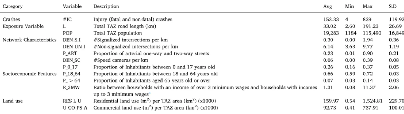
SIAT/FOR dataset provide information on fatal and non-fatal injury crashes as registered in the period from 2009 to 2011. These records were georeferenced according to the crash address by using the TransCAD5.0©software (Caliper, 2008). The database consolidation with all the information aggregated by the traffic zones, was carried out with the aid of standard GIS tools, such as functions that make it pos-sible to carry out a spatial search, superimposition of layers, and spatial operations based on the topological relationship of geographic entities. The explanatory variables used in the development of the models were divided into four categories: exposure, road network characteristics, socioeconomic features and land use, and their statistics are described, together with the frequency of injury crashes inTable 1.

The total road extension inside the traffic zone (L) and total TAZ Population (POP) were considered to represent the crash exposure. In other studies in the field (Aguero-Valverde and Jovanis, 2006; Hadayeghi et al., 2010; Li et al., 2013; Rhee et al., 2016), traffic volume was used as the exposure variable, usually in the VKT (Vehicle Kilo-meter Traveled) or DVMT (Daily Vehicle Miles Traveled) format; however, these variables are not available for this study.

have a greater exposure and, hence, a higher road crash risk. Socioeconomic features were regarded as risk factors, and the age and income of the residents in the traffic zones were available for this study. The variables representing the age of the inhabitants are the percentages of residents between 0 and 17 years old (proxyfor young pedestrians), between 18 and 64 years old (proxyfor drivers and pe-destrians) and percentage of the population 65 years old or over (proxy

for old drivers and pedestrians). The variable used to represent the income was the ratio between the number of households with income over 3 minimum wages and the number of households with an income below 3 minimum wages. A household with an income of over 3 minimum wages was regarded as a high-income household, and below this level as a low-income household. Thus, this variable indicates how often there are more households with a high income than a low income inside a particular zone.

The land use category has two variables: residential land use, (size per km2_{) and commercial land use (amount and service delivery per} km2). Different land use configurations in terms of activity as well as intensity, are likely to influence risk exposure to crashes for different types of road users.

The preliminary selection of the variables was based on the analysis of the dispersion and the correlation matrix involving each variable and the frequency of injury crashes. The DEN_UN_I variable was eliminated, because it did not show a considerable correlation with the crash fre-quency. The correlation matrix showed that many socioeconomic variables related to the age of the residents of the zones (P_0_17, P_18_64 and P_ > 64) were considerably correlated with each other; thus only P_ > 64 was chosen due to its higher correlation with the dependent variable.

The remaining explanatory variables had correlations with the crashes ranging from 0.19 (RES_L_U) to 0.53 (U_CO_PS_A), but the variables U_CO_PS_A, DEN_S_I and P_ART had higher correlations with each other than with the dependent variable. Three variable sets were created to avoid the inclusion of highly correlated variables, and these will be tested in the models, by encompassing one of the three variables (U_CO_PS_A, DEN_S_I and P_ART) and the remaining ones that were not eliminated (L, DEN_SC, R_3MW, P_ > 64andRES_L_U). In each set, the Variance Inflation Factor (VIF) was applied to assess multicollinearity and all the variables had a value lower than, or equal to,five, which indicates a moderate multicollinearity (Heiberger and Holland, 2015).

3.2. Coefficient estimation

GLM models of the Negative Binomial type were estimated for each selected non-collinear variable set, by choosing the model that had the best adjustment with regard to the ML and the AIC of all the sets. Given the considerably high correlation betweenLandPOP(0.88) these two

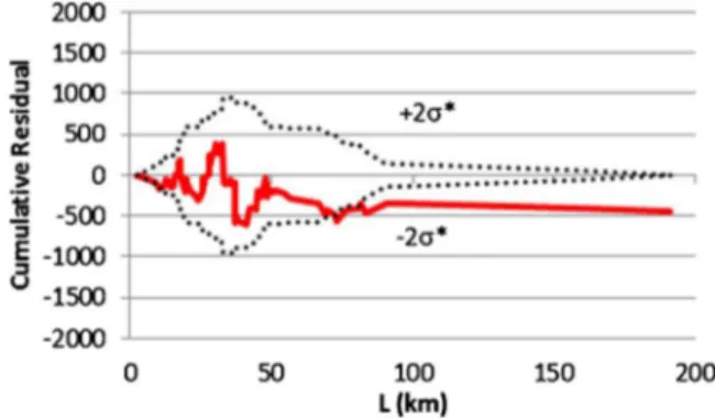
variables were tested separately in two global NB models. The pre-liminary tests suggested slightly better adjustments for the model with total TAZ Population with RMSE of 80.0 (as compared to 84.8), Log-likelihood of−1346 (as compared to−1378) and AICc of 1358 (as compared to 1391). The cumulative residual plot for the model with Population was outside the 2σ

denvelope for a wide range of Population (5000 to 22,000 inhabitants) when compared to the model based on road length (Figs. 1 and 2). Therefore, the total TAZ road extension (L) was selected to be the exposure variable, considering the similar results in terms of the RMSE, LL and AICc and its suitability in terms of model residuals (CURE plot).

The estimation of the geographically weighted spatial models (GWPR, GWNBRg and GWNBR) was carried out with a set of SAS/IML© macros developed bySilva and Rodrigues (2016). The advantage of using these macros is because the software GWR4, developed by Nakaya et al. (2012)and used to calibrate the GWPR, does not support the calibration of the geographically weighted regression model with the Negative Binomial structure.

By using SAS/IML macros, it was possible to determine the optimum bandwidth with the biquadratic adaptive and Gaussian fixed kernel functions, and the bandwidth that had the lowest AICc for the GWPR and GWNBRg models was chosen. In the case of the GWNBR, the de-finition of the optimum bandwidth, (whetherfixed or adaptive), used the CV optimization criterion, and the bandwidth that had the highest ML was chosen, since this parameter is a portion of the AICc, which was not possible to determine for the reasons set out in Section2.2.

In the case of the GWPR and GWNBRg models, the fixed kernel bandwidth provided slightly lower AICc, although the current TAZ configuration of Fortaleza has higher TAZ areas located close to the city border limits, mainly in the east and south. This makes the kernel function yield a sharper decay with the distance from afixed kernel bandwidth, and hence a small subsample will be considered for the calibration of these regions. However, this may also result in higher

Table 1

Descriptive statistics of the variables.

Category Variable Description Avg Min Max S.D

Crashes #IC Injury (fatal and non-fatal) crashes 153.33 4 829 119.92

Exposure Variable L Total TAZ road length (km) 33.02 2.60 191.23 26.69

POP Total TAZ population 19,283 1184 115,490 16,849

Network Characteristics DEN_S_I #Signalized intersections per km 0.30 0.00 1.94 0.36

DEN_UN_I #Non-signalized intersections per km 6.14 3.63 9.77 1.19

P_ART Proportion of arterial one-way and two-way streets 0.23 0.01 0.90 0.21

DEN_SC #Speed cameras per km 0.06 0.00 0.39 0.08

P_0_17 Proportion of Inhabitants between 0 and 17 years old 0.26 0.16 0.37 0.05 Socioeconomic Features P_18_64 Proportion of Inhabitants between 18 and 64 years old 0.66 0.59 0.72 0.03 P_ > 64 Proportion of Inhabitants aged 65 years old or over 0.07 0.03 0.14 0.03 R_3MW Ratio between households with an income of over 3 minimum wages and households with incomes

up to 3 minimum wagesa

1.31 0.08 11.37 2.06

Land use RES_L_U Residential land use (m2_{) per TAZ area (km}2_{) (x1000) 159.97 0.54 1,524.81 229.70}

U_CO_PS_A Commercial land use (m2_{) per TAZ area (km}2_{) (x1000) 92.73 0.41 737.91 100.01} a_{Minimum wage approximately US$ 300.00.}

standard errors for the coefficients, and for this reason the adaptive bandwidth was adopted for all the local models.

The estimations of the Negative Binomial and the geographically weighted models are shown inTable 2, as well as the descriptive sta-tistics of average, minimum and maximum values, 1st and 3rd quartile of the coefficients are given for the latter. By analyzingTable 2, it can be observed that the Negative Binomial regression coefficients, which are unique for the entire study area, had a positive impact on all the coefficients on the frequency of injury crashes.

InTable 2, the GWPR model shows average coefficients that are very different from the non-spatial global regression. On the other hand, it can be observed that the GWNBRg and GWNBR models had average values for the coefficients close to the Negative Binomial. The difference between the NB and GWPR coefficients is probably due to the fact that the GWPR does not take account of the overdispersion of the data.

Despite the fact that all the models provided positive average coefficients, the GWPR model had negative coefficients for some zones for the regression intercept and the P_ > 64, DEN_SC and DEN_S_I variables. The GWNBR model also had negative coefficients for the regression intercept, for P_ > 64 and DEN_S_I variables, and less TAZ than GWPR. It is worth noting that all the coefficients for all the vari-ables were positive for the GWNBRg model.

Counterintuitive signs for the coefficients found in the GWPR and GWNBR, may be due to the multicollinearity among the local coeffi-cients, rather than the required adjustment of the model to the more specific conditions of each region. The multicollinearity level among the coefficients can be estimated by means of the Variance Inflation Factor (Wheeler and Tiefelsdorf, 2005; Pirdavani et al., 2014).

The VIF estimates for the GWPR models were in the range of 1.03–1.51 and for the GWNBR models, in the range of 1.05–2.04 which indicates a low to moderate influence of the multicollinearity among the local coefficients. These results and the study of theFotheringham and Oshan (2016)spatial coefficient multicollinearity support the view that this issue may not be responsible for the counterintuitive signs.

Another reason for the appearance of counterintuitive signs may be the calibration base of the geographically weighted models. The hy-pothesis is that in certain zones, some variables may not be significant

and it is possible that local models produce counterintuitive signs for these variables (Haghayeghi et al., 2010;Pirdavani et al., 2014). Ac-cording toXu and Huang (2015), a failure to take account of the data overdispersion by the GWPR model, may cause unexpected signs of significant variable among the coefficients.

Figs. 3 and 4show the coefficients spatial distribution of the GWPR, GWNBRg and GWNBR models, as well as the overdispersion parameter (α_{) of the latter. By observingFigs. 3 and 4and comparing the same}

variable, it was found that the GWPR model has a higher number of zones with negative coefficients with regard to the GWNBR model. Out of the 126 zones, the P_ > 64, DEN_SC and DEN_S_I variables in the GWPR model showed negative signs in 42, 32 and 15 zones, respec-tively. And in the GWNBR model, for these same variables, they showed 17, 0 and 7 zones with altered signs, respectively, which suggests that a failure to take account of the overdispersion of the traffic crashes, may have caused more unexpected signs for the model coefficients.

The statistical significance of the coefficients was evaluated by means of tests developed bySilva and Fotheringham (2016), which are robust with regard to multicollinearity between the explanatory vari-ables (Fotheringham and Oshan, 2016). In the GWPR, the coefficients from P_ > 64 variable range between−59.37 and 35.35, and by ex-amining the significance of the zones with negative signs, it can be seen that 76% were not significant to a level of 10%. As for the GWNBR, the coefficient values of this variable have a lower variation, between −3.57 and 23.42, and all the zones with negative signs were not sig-nificant to a level of 10%.

The coefficients of the DEN_SC variable in the GWPR is also similar to the other variables, and they have a higher variation, with 100% of the zones showing non-significant negative signs. In the GWNBR, this variable did not have negative signs, and the significance level was 10%.

The DEN_S_I variable for the GWPR had coefficients ranging be-tween−1.59 and 17.10, and 73% of the zones that had negative signs were not significant with a significance level of 10%. In the GWNBR, this variable also had a lower variation of coefficients, between−0.55 and 5.43, and all the zones that had negative signs that were not sig-nificant.

Unlike the GWNBRg that used a global value of 0.23 for the over-dispersion parameter,Fig. 4 shows the spatial variation of this para-meter in the GWNBR.Fig. 4also shows thatαhad lower values in the

central and western regions and the values increased in the South and East direction of the city. These last regions have zones with heavy traffic in the streets, but are close to zones where there are still urban gaps or basically consist of local streets. The hypothesis is that these features make the GWNBR model yield higher values ofα for these

regions.

3.3. Adjustment measures and spatial dependency

The root mean squared error (RMSE), AICc and ML as explained before were applied to quantify and compare the performance of the models. The RMSE can be expressed as:

Fig. 2.Global NB Cure plot–Total road extension (L).

Table 2

–Negative Binomial, GWPR, GWNBRg and GWNBR model coefficients.

Coefficients NB GWPR GWNBRg GWNBR

β PV Avg Min Max Lwr Upr Avg Min Max Lwr Upr Avg Min Max Lwr Upr

Intercept 1.39 0.00 0.81 −2.73 3.22 0.01 1.83 1.39 0.69 2.00 1.18 1.60 1.10 −0.81 2.71 0.78 1.56

ln (L) 0.79 0.00 1.01 0.18 2.13 0.85 1.21 0.86 0.63 1.01 0.73 0.97 0.93 0.47 1.22 0.78 1.11 P_ > 64 8.28 0.00 4.80 −59.37 35.35 −1.77 11.63 6.62 2.47 10.18 4.62 8.46 6.40 −3.57 23.42 1.96 9.28

DEN_SC 2.58 0.00 1.62 −20.79 16.97 −0.03 2.58 2.17 1.10 3.76 1.50 2.76 2.27 0.29 7.85 1.06 3.13

DEN_S_I 0.43 0.02 2.31 −1.59 17.10 0.47 3.77 0.51 0.20 1.15 0.42 0.54 1.25 −0.55 5.43 0.55 1.37

∑

= −

RMSE

n y y

1

(observed predicted)2

(7) whereyobservedis the observed value of the dependent variable,ypredicted is the value predicted by the model andnis the size of the sample.

In addition to these metrics, the spatial dependency of the model was confirmed by determining the Moran Global Index (I) of the errors. The null hypothesis tested with Moran’s I is of independency or spatial randomness, which in this case would have the zero value. The Moran’s I varies between−1 and 1, where 0 (zero) value indicates the lack of a correlation. The closer it is to 1, the greater is the similarity between the neighbors and the stronger is the data concentration, and the closer it is to−1, the more dispersed is the data and lower is the similarity with

Fig. 3.Coefficients spatial distribution of the GWPR and GWNBRg models.

Fig. 4.Coefficients spatial distribution of the GWNBR models and overdispersion parameter (α).

Table 3

Adjustment measurements of the models of injury crashes.

Model Bandwidtha _{#Parameters RMSE 2LL AICc}

Negative Binomial – 5 84.8 −1378 1391

GWPR 14 78.4 19.8 −1222 1652

GWNBRg 98 13.0 60.7 −1345 1374

GWNBR 36 38.9b _41.0

−1237 –

a_{Number of neighbors;} b_{In this case, 1 was added to the e}

the neighbors.

Table 3shows the goodness of fit indicator for global and local models. The NB global model had the worst adjustments for the RMSE criteria and ML, followed by the GWNBRg, GWNBR and GWPR models. One hypothesis to explain why the two local GWNBRg and GWNBR models had a worse adjustment than the GWPR with regard to RMSE is that they are less vulnerable to extreme values, since their coefficients are smoother surfaces, and this can be observed from their larger bandwidth size as well as by the fact that they had a more homogeneous spatial variation of the coefficients than the GWPR model (Figs. 3 and 4).

With regard to the AICc, the best performance was the GWNBRg with a value of 1374, followed by the Negative Binomial and the GWPR, which had the worst result due to the high number of effective parameters, probably because they failed to take into account the overdispersion that exists in the crash data.

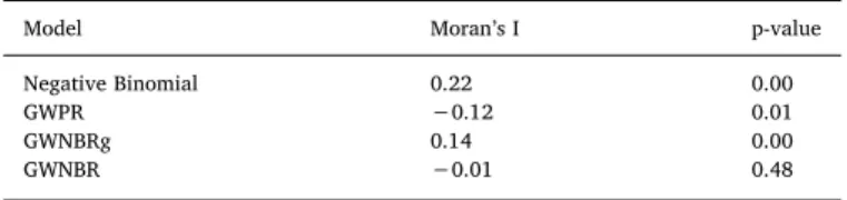
Table 4shows the comparison of the spatial autocorrelation values and the p-value for the estimated models. It should be noted that the GWPR and GWNBRg local models did not significantly reduce the spatial autocorrelation of the residuals, but the reduction was more expressive than the non-spatial NB model. This is probably due to possible model misspecification for the tested variables and the use of a constant value for the overdispersion parameter employed for the GWNBRg model (α= 0.23). There was a considerable reduction of the

residual autocorrelation for the GWNBR model with a significance level of 5%, which made it possible to reduce the data spatial heterogeneity and produce non-biased estimates to make a comparison with the NB, GWPR and GWNBRg models.

Tables 3 and 4allow an assessment to be made of the relationship between the model adjustment indicators and spatial dependency of the residuals. This spatial feature may not be directly related to model predictive power (RMSE/AIC). A very well adjusted global or local model does not guarantee a spatially non-biased model. A local model with non-spatially dependent residuals may be obtained at the expense of a slightly higher RMSE. This point is highlighted in this study. The GWNBR was the only model to significantly reduce the spatial de-pendency with a moderate RMSE, which was lower than the NB and GWNBRg model. The GWPR model yielded the lowest RMSE although it was not efficient enough to reduce the spatial dependency of the esti-mates.

When analyzing the spatial distribution of the coefficients for road length (L) for the GWNBR model, it was observed that the TAZs on the west side of the city incurred a higher risk per unit of extension than the zones on the east side. This apparent higher risk may reflect the fact that there are several arterial roads and, which are important traffic corridors and attract a large number of vehicles from the suburbs to the CBD. The west region also has a denser road network, unlike the east region that still has urban gaps since it has only recently been devel-oped.

The spatial distribution of the coefficients for variable P_ > 64 coefficients displays a very heterogeneous pattern for the GWPR model, with higher values in the northern part of the city and several inter-mediate zones with negative coefficients. In the case of the GWNBRg model, the spatial variation of the coefficients is more homogeneous, and it is smaller in the center/northwest, becoming gradually higher as one moves towards the southeast. With regard to the GWNBR model,

the center/north-west regions had the lowest coefficients, however with a group of zones with non-significant negative coefficients, followed by a growth in the south-west direction. In the southeast direction there is also a growth in the coefficients and then another area of low non-significant values in the outskirts of the city.

The GWNBRg and GWNBR models provide a spatial distribution of coefficients for the DEN_SC and DEN_S_I variables that is more homo-geneous, unlike the GWPR. The lowest coefficients are in the northern region, where most of the signalized intersections and speed cameras are concentrated, and crashes result in less severe injuries. There is a gradual increase in the coefficients which probably reflects the increase of crashes involving injuries. This caused by the higher speeds in the streets in the southern district, since there are few signalized intersec-tions and speed cameras in this area.

4. Concluding remarks

This study investigated the use of four different strategies for safety for the estimation of crash frequency aggregated at the traffic zone level. A comparative analysis was carried out for a non-spatial model of the GLM type with Negative Binomial distribution, a local spatial Geographically Weighted Poisson Regression (GWPR) model and two types of Geographically Weighted Negative Binomial Regression (GWNBRg and GWNBR) models based on a case study undertaken in Fortaleza, Brazil.

The estimated models to determine the frequency of injury crashes use explanatory variables of a socioeconomic kind, with demographic, land use and road network features, aggregated in traffic zones. The GWPR model had a higher frequency of TAZ with counterintuitive signs than the GWNBR. The model coefficients of GWPR showed greater heterogeneity than GWNBR and GWNBRg, and the hypothesis is that this occurred because the GWPR does not include overdispersion of crash data and has a significantly lower bandwidth and thus sharp coefficient surfaces.

The GWPR model yielded both the lowest root mean squared error (RMSE) and the maximum likelihood, when compared with the other models. The low RMSE is caused by the observed coefficient hetero-geneity of the GWPR and hence a greater adjustment to extreme values as compared to the GWNBR approach. The GWNBRg model had a better adjustment, when the AICc are taken into account, followed by the GWPR model.

Despite its apparent superior adjustment for RMSE and maximum likelihood, it was not possible to remove the global spatial dependency of the residuals from the GWPR model. In addition, the GWNBRg failed to eliminate the residual spatial dependency probably owing to the use of a constant value for the overdispersion parameter. The GWNBR was the only approach that was able to capture the spatial heterogeneity between the frequency of injury crashes and the explanatory variables, since it reduced the spatial dependency of the model residuals.

The results of this study support the use of the GWNBR as a pro-mising tool for safety planning, especially because it makes it possible to model non-stationary spatially counting data that show over-dispersion. However, this technique needs further investigation to provide a more robust method for making a comparison between the models (AICc is not possible at this stage). Moreover, the use of the cross validation method to determine the optimum bandwidth may increase the risk of overfitting; that is, the model might adjust so strongly to the existing data that it will lose its predictive capacity for crash estimation in a new dataset. Furthermore, in situations where specific variables do not show a clear spatial variation, it may be worth designing semi-parametric models, although unfortunately these types of models are still not available for the GWNBR.

One limitation of this work is the absence of trafficflow, which is usually one of the most important variables used to capture traffic ex-posure. However this variable is often not available or is given as a result of a four-step transportation modeling system. Another factor

Table 4

Residues spatial dependency of the estimated models (Moran Global Index).

Model Moran’s I p-value

Negative Binomial 0.22 0.00

GWPR −0.12 0.01

GWNBRg 0.14 0.00

that requires further attention is the possible influence of the relatively small sample size (126 TAZs) of this study with regard to the RMSE and in particular, the maximum likelihood estimates (especially for the GWNBR model).

To the best of our knowledge, this research study is one of thefirst applications of the GWNBR model to thefield of road safety. It is be-lieved that the application of this type of approach can be re-commended for different datasets, especially for an analysis of a larger number of traffic zones to confirm the underlying assumptions and results obtained from this research endeavor. Furthermore, to increase the applicability of these models for transport planning, it is important to investigate their temporal transferability in the same area (model validation).

Acknowledgments

The authors would like to acknowledge the Brazilian National Council for Scientific and Technological Development (CNPq), and the Ceará State Foundation for Scientific and Technological Development (FUNCAP) for funding this research.

References

Abdel-Aty, M., Lee, J., Siddiqui, C., Choi, K., 2013. Geographical unit based analysis in the context of transportation safety planning. Transp. Res. Part A Policy Pract. 49, 62–75.

Aguero-Valverde, J., Jovanis, P.P., 2006. Spatial analysis of fatal and injury crashes in Pennsylvania. Accid. Anal. Prev. 38, 618–625.

Cai, Q., Lee, J., Eluru, N., Abdel-Aty, M., 2016. Macro-level pedestrian and bicycle crash analysis: incorporating spatial spillover effects in dual state count models. Accid. Anal. Prev. 93, 14–22.

Caliper, 2008. TransCAD–Transportation Workstation Software, User’s Guide, Version 5.0 for Windows. Caliper Corporation, Newton, USA.

Chatterjee, A., Wegmann, F., Fortey, N., Everett, J., 2001. Incorporating safety and se-curity issues in urban transportation planning. In: A Paper Presented at the 80th Annual TRB Meeting. Washington, D.C.

Chen, V.Y.J., Yang, T.C., 2012. SAS macro programs for geographically weighted gen-eralized linear modeling with spatial point data: applications to health research. Comput. Methods Programs Biomed. 107, 262–273.

Dumbaugh, E., Meyer, M.D., Washington, S., 2004. Incorporating sate highway safety agencies into safety-Conscious planning process. In: A Paper Presented at the 83th Annual TRB Meeting. Washington, D.C.

Erdogan, S., 2009. Explorative spatial analysis of traffic accident statistics and road mortality among the provinces of Turkey. J. Saf. Res. 40, 341–351.

Farber, S.E., Páez, A., 2007. A systematic investigation of cross-validation in GWR model estimation: empirical analysis and Monte Carlo simulations. J. Geog. Syst. 9, 371–396.

Fotheringham, A.S., Oshan, T.M., 2016. Geographically weighted regression and multi-collinearity: dispelling the myth. J. Geogr. Syst. 18 (4), 303–329.

Fotheringham, A.S., Brunsdon, C., Charlton, M.E., 2002. Geographically Weighted Regression: the Analysis of Spatially Varying Relationship. Wiley, Chichester. Hadayeghi, A., Shalaby, A.S., Persaud, B.N., 2003. Macro-level accident prediction

models for evaluating safety of urban transportation systems. Transp. Res. Rec. 1840 (1), 87–95.

Hadayeghi, A., Shalaby, A.S., Persaud, B.N., 2010. Development of planning level transportation safety tools using Geographically Weighted Poisson Regression. Accid.

Anal. Prev. 42, 676–688.

Heiberger, R.M., Holland, B., 2015. Statistical Analysis and Data Display–an Intermediate Course with Examples in R, 2nd edition. Springer (eBook). Huang, H., Xu, P., Abdel-Aty, M., 2013. Transportation safety planning: a spatial analysis

approach. TRB 92th Annual Meeting (TRB 2013-1855).

ITE, 2009. Transportation Planning Handbook, 3rd edition. Institute of Transportation Engineers.

Lee, J., Abdel-Aty, M.E., Jiang, X., 2014. Development of zone system for macro-level traffic safety analysis. J. Transp. Geogr. 38, 13–21.

Li, Z., Wang, W., Liu, P., Bigham, J.M., Ragland, D.R., 2013. Using geographically weighted Poisson regression for county-level crash modeling in California. Saf. Sci. 58, 89–97.

Lord, D., Persaud, B.N., 2004. Estimating the safety performance of urban road trans-portation networks. Accid. Anal. Prev. 36 (4), 609–620.

Lovegrove, G.R., Sayed, T., 2006. Macro-level collision prediction models for evaluating neighbourhood traffic safety. Can. J. Civ. Eng. 33, 609–621.

Matkan, A.A., Mohaymany, A.S., Mirbagheri, B., Shahri, M., 2011. Explorative spatial analysis of traffic accidents using GWPR model for urban safety planning. In: 3rd International Conference on Road Safety and Simulation. September 14–16, 2011, Indianapolis, USA.

Nakaya, T., Fortheringham, A.S., Brunsdon, C., Charlton, M., 2005. Geographically Weighted Poisson regression for disease association mapping. Stat. Med. 24, 2695–2717.

Nakaya, T., Charlton, M., Lewis, P., Fortheringham, S., Brunsdon, C., 2012. Windows Application for Geographically Weighted Regression Modeling. Ritsumeikan University, Kyoto, Japan.

Pirdavani, A., Bellemans, T., Brijs, T., Wets, G., 2014. Application of geographically weighted regression technique in spatial analysis of fatal and injury crashes. J. Transp. Eng. 140 (8).

Pulugurha, S.S., Duddu, V.R., Kotagiri, Y., 2013. Traffic analysis zone level crash esti-mation models based on land use characteristics. Accid. Anal. Prev. 50, 678–687. Quddus, M.A., 2008. Modeling area-wide count outcomes with spatial correlation and heterogeneity: an analysis of London crash data. Accid. Anal. Prev. 40, 1486–1497. Rhee, K.A., Kim, J.K., Lee, Y., Ulfarsson, G.F., 2016. Spatial regression analysis of traffic

crashes in Seoul. Accid. Anal. Prev. 91, 190–199.

Siddiqui, C., Abdel-Aty, M., Choi, K., 2012. Macroscopic spatial analysis of pedestrian and bicycle crashes. Accid. Anal. Prev. 45, 382–391.

Silva, A.R., Fotheringham, A.S., 2016. The multiple testing issue in geographically weighted regression. Geogr. Anal. 48, 233–247.

Silva, A.R., Rodrigues, T.C.V., 2014. Geographically weighted negative binomial regres-sion-incorporating overdispersion. Stat. Comput. 24, 769–783.

Silva, A.R., Rodrigues, T.C.V., 2016. A SAS. (Available at: <http://support.sas.com/ resources/papers/proceedings16/8000-2016.pdf>).

Song, B., Huang, H., Zeng, Q., Deng, Q., Abdel-Aty, M., 2015. Comparative analysis of macro and micro models for zonal crash prediction. TRB 94th Annual Meeting (n. 15-2774).

Tarko, A.P., Inerowicz, M., Ramos, J., Li, W., 2008. Tool with road-level crash prediction for transportation safety planning. Transp. Res. Rec.: J. Transp. Res. Board 2083 (1), 16–25.

Tarko, A.P., 2006. Calibration of safety prediction models for planning transportation networks. Transp. Res. Rec.: J. Transp. Res. Board 1950 (1), 83–91.

Wang, X., Yang, J., Lee, C., Ji, Z., You, S., 2016. Macro-level safety analysis of pedestrian crashes in Shanghai, China. Accid. Anal. Prev. 96, 12–21.

Wheeler, D., Tiefelsdorf, M., 2005. Multicollinearity and correlation among local re-gression coefficients in geographically weighted regression. J. Geogr. Syst. 7 (2), 161–187.

Xu, P., Huang, H., 2015. Modeling crash spatial heterogeneity: random parameter versus geographically weighting. Accid. Anal. Prev. 75, 16–25.

Xu, P., Huang, H., Dong, N., Wong, S.C., 2017. Revisiting crash spatial heterogeneity: a bayesian spatially varying coefficients approach. Accid. Anal. Prev. 98, 330–337. Yu, C., Xu, M., 2017. Local variations in the impacts of built environments on traffic