the Least-Action Principle
Nedialko I. Krouchev1*, Simon M. Danner2,3, Alain Vinet4, Frank Rattay2, Mohamad Sawan1
1Polystim Neurotechnologies, Ecole Polytechnique, Montreal, Quebec, Canada,2Institute for Analysis and Scientific Computing, University of Technology, Vienna, Austria,3Center for Medical Physics and Biomedical Engineering, Medical University, Vienna, Austria,4Institut de Genie Biomedical, Universite de Montreal, Montreal, Quebec, Canada
Abstract
Electrical stimulation (ES) devices interact with excitable neural tissue toward eliciting action potentials (AP’s) by specific current patterns. Low-energy ES prevents tissue damage and loss of specificity. Hence to identify optimal stimulation-current waveforms is a relevant problem, whose solution may have significant impact on the related medical (e.g. minimized side-effects) and engineering (e.g. maximized battery-life) efficiency. This has typically been addressed by simulation (of a given excitable-tissue model) and iterative numerical optimization withharddiscontinuous constraints - e.g. AP’s are all-or-none phenomena. Such approach is computationally expensive, while the solution is uncertain - e.g. may converge to local-only energy-minima and be model-specific. We exploit theLeast-Action Principle(LAP). First, we derive in closed formthe generaltemplateof the membrane-potential’s temporal trajectory, which minimizes the ES energy integral over time and overanyspace-clamp ionic current model. From thegivenmodel we then obtain thespecificenergy-efficient current waveform, which is demonstrated to beglobally optimal. The solution is model-independent by construction. We illustrate the approach by a broad set of example situations with some of the most popular ionic current models from the literature. The proposed approach may result in the significant improvement of solution efficiency: cumbersome and uncertain iteration is replaced by a single quadrature of a system of ordinary differential equations. The approach is further validated by enabling a general comparison to the conventional simulation and optimization results from the literature, including one of our own, based on finite-horizon optimal control. Applying the LAP also resulted in a number of general ES optimality principles. One such succinct observation is that ES with long pulse durations is much more sensitive to the pulse’s shape whereas a rectangular pulse is most frequently optimal for short pulse durations.
Citation:Krouchev NI, Danner SM, Vinet A, Rattay F, Sawan M (2014) Energy-Optimal Electrical-Stimulation Pulses Shaped by the Least-Action Principle. PLoS ONE 9(3): e90480. doi:10.1371/journal.pone.0090480
Editor:Dante R. Chialvo, National Research & Technology Council, Argentina
ReceivedNovember 11, 2013;AcceptedJanuary 30, 2014;PublishedMarch 13, 2014
Copyright:ß2014 Krouchev et al. This is an open-access article distributed under the terms of the Creative Commons Attribution License, which permits unrestricted use, distribution, and reproduction in any medium, provided the original author and source are credited.
Funding:The Fonds de recherche du Quebec - Nature et technologies and the Natural Sciences and Engineering Research Council of Canada provided funding for this work. S.D. was supported by the Vienna Science and Technology Fund (WWTF), Proj.Nr. LS11-057. The funders had no role in study design, data collection and analysis, decision to publish, or preparation of the manuscript.
Competing Interests:The authors have declared that no competing interests exist.
* Email: [email protected]
Introduction
Electrical stimulation (ES) today is an industry worth in excess of 3 G$. ES devices interact with living tissues toward repairing, restoring or substituting normal sensory or motor function [1]. The rehabilitation-engineering applications scope is constantly growing: from intelligent limb prosthetics and deep-brain stimu-lation (DBS) to bi-directional brain-machine interfaces (BMI), which are no longerjustabout recording brain activity, but have also recently used ES towardclosed-loopsystems, [2–5].
Application-specific current patterns need to be injected toward reliably elicitingaction potentials(AP’s) in target excitable neural tissue. To prevent tissue damage or loss of functional specificity, the employed current waveforms need to beefficient. This may significantly impact the biomedical effects and engineering feasibility. Hence, an optimization problem of high relevance to the design of viable ES devices is to minimize the energy required by the stimulation waveforms, while maintaining their capacity for AP triggering toward achieving the targeted functional effects.
A number of recent studies of ES optimality are based on extensive model simulation and related numerical methods
through the wider spread of high-performance computing, e.g. [6–9]. The model dynamics to iterate can be arbitrarily complex and nonlinear. This implies lengthy numerically-intensive compu-tation, irregular convergence and constraints that may be difficult to enforce - e.g. that an AP is anall-or-nonephenomenon. Thus, any function of membrane voltage will suffer dramatic disconti-nuities at parameter-space manifold boundaries where intermit-tent AP’s are likely to be elicited.
Hence, such an iterative approach is not only computationally expensive, but its solution quality is highly uncertain and model-specific. The long-lasting iteration may converge to shallow local energy-minima. Such numerical misdemeanor of the approach is well known to its frequent users.
In this work we follow the ES pioneers - we use physical reasoning and related mathematics toward a more theoretical treatment of the subject.
experiments with multiple physiological preparations [13,14]. This classical work led to concepts like strength-duration curve (SD), i.e. the function of threshold (but still AP-evoking) ES current strength on duration. The first mathematical fit to this empirical results is usually attributed to Weiss, [10,15]
ITHR(T)~b(1zc=T) ð1Þ
where T is the stimulus duration, b is called the rheobase (or rheobasic current level) andcis thechronaxie.
The most expedite way of introducing the rheobase and chronaxiewould be to point to eqn. (1) and notice that:
lim
T??ITHR(T)
~b ð2Þ
and
ITHR(c)~2b ð3Þ
i.e. the rheobase is the threshold current strength with very long duration, and chronaxie is the duration with twice the rheobasic current level. In the pioneering studies electrical stimulation was done with extracellular electrodes.
Eqn. (1) is the most simplistic of the 2 ‘simple’ mathematical descriptors of the dependence of current strength on duration, and leads to Weiss’ linear charge-transfer progression with T,
Q(T)~T|ITHR~b|(Tzc): Both Lapicque’s own writings -[11–13], and more recent work are at odds with the linear-charge approximation. Already in 1907 Lapicque was using a linear first-order approximation of the cell membrane, modeled as a single-RC equivalent circuit with fixed threshold:
ITHR(T)~ b
1{e{T=t~bz be{T=t
1{e{T=t ð4Þ
with time constant t~C=g;C and g~1=R are the membrane capacity and conductance respectively.
The second form of eqn. (4) is easily obtained by subtracting/ adding the term be{T=t. From it, when t
&T (and hence
e{T=t?1):
ITHR(T)&b(1zt=T)
which accounts for the hyperbolic shape of the classic Lapicque SD curve.
Originally, eqn. (4) described the SD relationship for extra-cellular applied current. However, the single-RC equivalent circuit with fixed threshold, where I is the electrode current flowing across the cell membrane
Cvv_zv=R~I ð5Þ
can be used with either extra- or intra-cellular stimulation.
v~(V{Vrest) is the reduced membrane voltage with Vrest the restingvalue ofV:From eqns. (4) and (5), one may also see that
b~g(VTHR{Vrest), where VTHR is the attained membrane voltage at the end of the stimulation (at timeT).
Notice that the chronaxiecis not explicitly present in eqn. (4). Notice also that - with very short durationT%t,by the Taylor series decomposition of the exponent (around T~0), one may have either ITHR(T)&bt=T or ITHR(T)~b½1zt=T:Note that these two different simplifications (and esp. the latter) are
‘historical’ and depend on which of the two right-hand sides (RHS’) of eqn. (4) is used. In the second case only the denominator is developed to first order, while the numerator is truncated at zero-order. The second approximation throws a bridge to Weiss’ empirical formula of eqn. (1). I.e. the latter is a simplification of a simplification (i.e. of the 1st-order linear membrane model), capturing best the cases of shortest duration. On the other hand,
ITHR(T)&bt=T leads to a constant-charge approximation. Interestingly, the latter may fit well also more complex models of the excitable membrane, which take into account ion-channel gating mechanisms, as well as intracellular current flow, which may be the main contributors for deviations from both simple formulas. These ‘subtleties’ are all clearly described in Lapicque’s work, but less clearly by one of the most recent accounts in [16]. Before we continue, it is in order to examine the practical value of numerical optimization to identify energy-efficient waveforms. It is limited for the following reasons. First, it is subject to the rigorous constraints ofquantitativeequivalence between the model used and the real preparation to which the results should apply. A noteworthy example is provided by the very practice of numerical simulations: often a minute change in parameters precludes the use of ajust computedwaveform, which is no longer able to elicit an AP in the targeted excitable model. Alas, the same or similar applies hundredfold to the real ES practice.
Second, in the search for minimum-energy waveforms, using numerical mathematical programming algorithms, there is no guarantee about obtaining a globally optimal solution.
Finally, such an approach sheds very little light with respect to the major forces that are at play, and the key factors which determine excitability, such as - for example, the threshold value of membrane potential, whose crossing triggers an AP.
However, the problem at hand is also reminiscent of the search for energy-efficiency in many other physical domains - e.g. ecological car driving. For centuries, physics has tackled similar problems through an approach known as the Least-Action Principle(LAP) [17].
Thus, we first used simple models to derive key analytical results. We then identified generally applicable optimality princi-ples. Finally, we demonstrate how these principles apply also to far more complex and realistic models and their simulations.
The modeling and algorithmic part of this work is laid out in the next section. First, we introduce a simple and general model template. Next we present four most popular specific ionic-current models. Each of these can bepluggedin the template to describe an ES target in a single spatial location in excitable-tissue (or alternatively - a space-clamped neural process).
We then examine the conditions for the existence of a finite membrane-voltage threshold for AP initiation. The introduced ionic-current model properties are analyzed to gain important insights into the solution of the main problem at hand.
Two very different ways to identify energy-efficient waveforms are presented in the last two subsections of the Methods. The first relies on a standard numerical optimal-control (OC) approach. The second outlines the LAP in its ES form, which is used to derive a general analytic solution for the energy-optimal trajec-tories in time of the membrane-potential and stimulation-current. The Results section presents the model-specific results, applying OC or the LAP. We perform a detailed optimality analysis for both the simple and more realistic models. Comparisons between the two types of approaches, and the quality of their solutions, are made.
Methods
A General Excitability Model Template
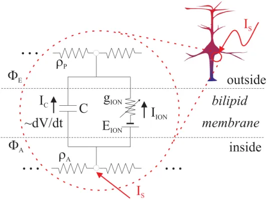
For the equivalent circuit of Fig. 1,ISis the stimulation current. IC is the capacitive current, whose direction is as shown on the Figure when the excitable-membrane’s potential is being depolar-ized. The algebraic sum of all the ionic and all axial currents is represented by IS~IIONzIaxial, where Iaxial stands for the algebraic difference (divergence) of in- and out-going axial currents. In the sequel we will use the notation u(t)~IS(t) for the stimulation-current waveform. The latter is oursystem input, which will be the leverage to refine in order to achieve desirable outcome - reliable triggering of APs in the excitable system. It is customary in the control literature to denote such a signalu(t):
Thus, all the currents are linked by the first Kirchhoff circuit law:
u(t):IS(t)~IC(t)zIS½V(t),x(t)~CmVV_zIS(V,x) ð6Þ
where - in the most general form, IS depends on membrane
voltage V(t) and on the state vector of the ionic channels’ gate
variables. Unless ambiguous, below we will simplify notation by writingIS(V):
Cm (typically around 1mF=cm2, [18]) andV(t) (inmV’s) are the excitable-membrane’s capacitance and potential. Equation (6) can be rewritten as:
CmVV_~u(t){IS(V) ð7Þ
Clearly according to eqn. (7), an outgoing total ionic current opposesthe effects of cathodic stimulation, since not all ofu(t)is employed toward the main goal of maximizing theV(t) growth, which the reader may have also already deduced from the equivalent circuit of Fig. 1. Conversely, ingoing total currentassists the effects of stimulation. Hence, in such a caseu(t)may belower
Table 1.Commonly used abbreviations.
Symbol Description
0D zero-dimensional, i.e. single-compartment or space clamp models; whose spatial extents are confined to a point
1D cable-like, multi-compartment spatial structure; homo-morphic to line
2D etc. two- or more dimensional, refers to the number of states that describe the excitable system’s dynamics
AIS the axon’s initial segment
AP Action potential
ASA Adjoint Sensitivity Analysis
BCI brain-computer interface
BMI brain-machine interface
BVP Boundary-value [ODE solution] problem
BVDP the Bonhoeffer-Van der Pol oscillator-dynamics model; also known as the Fitzhugh-Nagumo model
DBS Deep-brain stimulation
ES Electrical stimulation
FHOC Finite-Horizon Optimal-Control
FP Fixed point of system dynamicsRvanishing derivative(s)
HH or HHM Hodgkin and Huxley’s [model of excitable membranes]
IM the Izhikevich model
LM the Linear sub-threshold model; also known in computational neuroscience as leaky integrate & fire
MRG the McIntyre, Richardson, and Grill model
OC Optimal-Control
ODE Ordinary Differential equation; see also PDE
PDE Differential equation involving partial derivatives; see also ODE
LAP the Least-Action Principle
RN Ranvier-node
RHS right-hand side
SD strength-duration[curve]
W.R.T. with respect to
doi:10.1371/journal.pone.0090480.t001
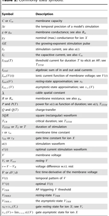
Table 2.Commonly used symbols.
Symbol Description
CorCm membrane capacity
Dt the temporal precision of a model’s simulation
gorgm membrane conductance; see alsoRm
gX nominal (max.) conductance for ionX
GE the growing-exponent stimulation pulse
IS stimulation current, see alsou(t)
IC the capacitive current, see alsoCm
ITHR(T) threshold current for durationTto elicit an AP; see TSTIM
Iaxial algebraic sum of in and out axial currents
Iion(V(t)) ionic current function of membrane voltage; seeV(t)
Iion,0(V) resting-state approximation; seex0
Iion,?(V) asymptotic-state approximation; seex?(V)
cable spatial constant
RorRm membrane resistance; see alsogm
PandP(T) power foru(t)as function of duration; seeu(t),TSTIM
QandQ(T) charge-transfer
SQR square (rectangular) waveform
TCR critical duration; seeTSTIM
TSTIMorTSorT duration of stimulation
tortm membrane time constant
tionortX gate time constant for ionX
u(t) stimulation waveform
u(t) optimal current stimulation waveform
V membrane voltage
VrorVrest restingV
v~V{VR voltage difference w.r.t. rest
_
V
VordV=dt first time-derivative of the membrane voltage
V(t) temporal pattern ofV
V(t) optimalV(t)
VTHR AP triggeringVthreshold
VTHR,0 resting-stateVTHR
VTHR,? theasymptotic-stateVTHR
x0~x?(Vr) gaterestingstate for ionX; seeVr
x?(V)~limt??x(tjV) gateasymptoticstate for ionX
than when it is estimated assuming the absence of membrane conductivity. Let us elucidate right away by providing typical examples.
Specific Single-compartment (Space-clamp) Models The models here are zero-dimensional (0D). Their spatial extents are confined to a point. This may be contrasted to the multi-compartment cable-like models that we will discuss later, and whose spatial structure is one-dimensional (1D)- i.e. homo-morphic to a line.
For single-compartment models there are no axial currents. Hence,IS~IION.
Linear Sub-threshold model (LM).
IION(V)~gm(V(t){Vr) ð8Þ
gm is the excitable-membrane’s resting (V~Vr~270 mV) conductance - in milli-Siemens per unit membrane surface area - e.g. 1mS=cm2. SubstitutingI
ION(V)from eqn. (8) into eqn. (6) yields a linear first-order model with t~Cm=gm~RmCm the familiar expression for the time constant of such a dynamic model. This model predicts a reasonable restingt&1ms.
As pointed out in the introduction, this type of model was extensively used by the ES pioneers, [12]. They were particularly concerned with the derivation of analytic expressions for the experimentally observed strength-duration (SD) curves. The latter describe the threshold (minimal) current strength (ITHR), which if maintained constant (i.e. through a rectangular waveform) for a given duration T is
likely to elicit an AP in excitable-tissue (see the introductory section).
Even if it may account for a significant part of the sub-threshold variation of the membrane’s potential, the linear model lacks a paramount feature - it cannot fire AP’s as the latter are due to the highlynonlinearproperties of the excitable-membrane’s conduc-tance around and beyond the firing threshold.
The Hodgkin-Huxley-type model (HHM). Hodgkin and
Huxley (HH) not only proposed a novel way to model ionic-channels but also introduced ionic-channel-specific parameters to fit experimental data [19]. Since, HH-type models have been proposed for many ionic-channels for cardiac to neuroscience applications.
We present one such model from the literature - [20], which has been used to fit experimental data from the central nervous system and particularly theneocortex.
IION(V,x)~gNam3h(V{ENa)zgKn(V{EK)
zgleak(V{Eleak)
ð9Þ
See Tables 3 and 4, which define all the model’s variables and parameter values. We consider specifically the Naz
v1:6 sodium
channel subtype, to which the axon initial segment (AIS) owes its higher excitability [20,21].
The dynamics of a gate-state variablex(t)(wherex(t)stands for one ofm(t),h(t),n(t)) are described by:
Figure 1. Excitability modeltemplate: The equivalent circuit represents the simplified electro-dynamics of an excitable membrane.
ISis the intra-cellular stimulation current.IC~CVV_ is the capacitive current. The direction of the latter is for a case ofdepolarizingthe membrane’s
voltage (i.e. the inside of the cell wall becoming more positive). The algebraic sum of all the ionic and all axial currents is represented by IS~IIONzIaxial,whereIaxialstands for the algebraic difference (divergence) of in- and out-going axial currents.
tx(V)xx_zx~x?(V) ð10Þ
Eqns. (6), (9) and (10) define a system of four coupled ODE’s -with respect to the four dynamic variables½V,m,h,n(t).
Further simplification may reduce the model complexity, maintaining only V(t) as the single dynamic variable. Gate-variable states are factored out by introducing appropriate non-dynamic functions of the membrane potential. E.g. in eqn. (9), the fast m gates may be assumed to reach instantaneously m?(V), while the far slowerhandngates remain at their resting values (corresponding to a membrane at its resting equilibrium potential
Vr).
The Izhikevich model (IM).
IION(V,w)~w{0:04V2{5V{140 ð11Þ
This model [22] has a second-order nonlinearity, compared to its predecessor - the BVDP model [23], which contains a cubic nonlinearity. The IM will therefore not auto-limit. As in the BVDP, there is a slow second dynamic variable w(t) called the ‘recovery current’ and its dynamics is described by:
_ w
w=c~bv{w ð12Þ
The IM responds to supra-threshold stimulation with a wide variety of AP-firing patterns, depending on the particular choices of parameters. Interested in the sub-threshold regimen, we have chosen the ‘‘Spike Latency’’ set: b~0:2,c~0:02 [24]. Hence,
tw~1=c is equal to 50 ms. At the time-scale of a single stimulation pulse (lasting at most a few milliseconds),wis virtually a constant.
Here, it may be important to remind the reader that the state of simplest models like the IM needs to be artificiallyreset after an AP event. However in more complex models (e.g. the HHM), channels that are responsible to revert the system to its resting potential will have a significant effect on the optimal waveform. We will see this in more detail in the results section.
Multi-compartment Models
To expand the scope of our analysis and the applicability of its results, it is essential to also address models of AP initiation and propagation along spatial neural structures. A popular example is the McIntyre, Richardson, and Grill model (MRG002). It was originally used to simulate the effects of ES
in the peripheral nervous system and specifically the myelin-ated axons that form nerve bundles [25]. An adapted version of the same model was recently used to simulate the effects of DBS [7].
Myelinated axon has been pinpointed as the most excitable tissue with extracellular stimulation [26–28]. Therefore models like the MRG’02 are of particular interest. Moreover, this model facilitates the illustration of optimality principles as it has only one excitable compartment type - the Ranvier-nodes (RN). The paranodal and other compartments that form the myelinated internodal sections are all modeled as a passive double-cable (due to the myelin sheath that insulates the extracellular periaxonal space) structure, see Fig. 2.
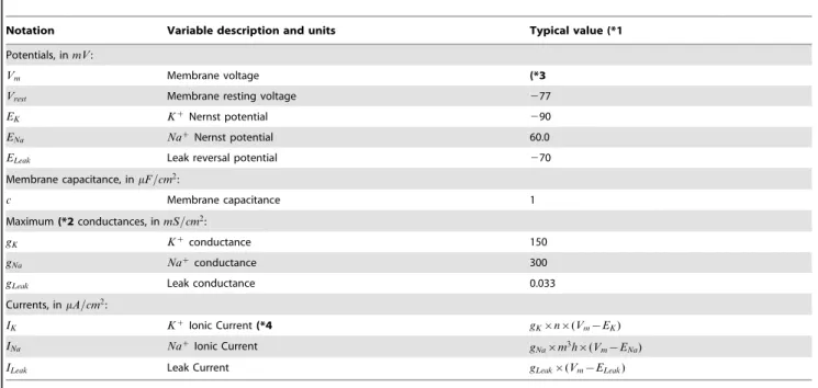
Table 3.Definition and notation for the key HHM variables.
Notation Variable description and units Typical value (*1
Potentials, inmV:
Vm Membrane voltage (*3
Vrest Membrane resting voltage 277
EK Kz
Nernst potential 290
ENa NazNernst potential 60.0
ELeak Leak reversal potential 270
Membrane capacitance, inmF=cm2:
c Membrane capacitance 1
Maximum(*2conductances, inmS=cm2:
gK Kzconductance 150
gNa Nazconductance 300
gLeak Leak conductance 0.033
Currents, inmA=cm2:
IK KzIonic Current(*4 gK|n|(Vm{EK)
INa NazIonic Current
gNa|m3h|(Vm{ENa)
ILeak Leak Current gLeak|(Vm{ELeak)
Notes:
(*1Typical values are for theNav1:6model, [20]; see also Table 4.
(*2These are dependent on (grow with) temperature, the values listed are forT~230 C.
(*3Membrane voltage is either at its resting valueVrest; is depolarized (grows due to stimulation and/or activated sodiumNazion channels); is repolarized (decays back toVrest, due to the potassiumKzion channels).
The RN compartment is a model of the HH-type:
Iion(V,x)~gNa,fm3h(V{ENa)zgNa,pp3(V{ENa)
zKn4(V{E
K)z leak(V{Eleak)
ð13Þ
Here two different Naz
ion channel subtypes are modeled (please see Table 5 for all the details). The fast subtype (with maximum conductance parameter gNa,f) is controlled by the openingmand closinghgate states. Thepersistentsubtype (with maximum conductancegNa,p) is controlled by thepgates. As its name suggests, it has no gate-inactivating states and is
non-inactivating. In addition, this model has very slow s gates, associated to itsKz
ion channel andveryfastmgates.
Below we call a fixed point (FP) every VFP value s.t. IION(VFP)~0. From eqn. (7) withu~0,
_ V V
VFP~0
The nonlinear dynamics behavior of the RN compartment taken in isolation is quite unlike that of the specific single-compartment HHM example we provided above. None of its four FPs are stable. Around itsunstable‘resting’ state (Vr=280mV), the zero-dimensional RN’s of MRG’02 model yielddepolarizing
Table 4.Gate-state dynamics parameters.
Notation Variable description Value
Temperature dependence:
Q10 Q10constant(*1 2.3
Kz
:n-gate(*2
an n-gate max opening rate 0.02
bn n-gate min closing rate 0.002
Vn,1=2 half-min/max in/activation rate voltage 25mV
kn n-gate voltage constantk 9
Naz
v1:6:m-gate(*2
am m-gate max opening rate 0.182
bm m-gate min closing rate 0.124
Vm,1=2 half-min/max in/activation rate voltage 41mV
km m-gate voltage constantk 6
Naz
v1:6:h-gate(*2
ah h-gate max opening rate 0.024
bh h-gate min closing rate 0.0091
Vh,1=2,a half-max activation rate voltage 48mV
Vh,1=2,b half-min inactivation rate voltage 73mV
kh h-gate voltage constantk 5
kh,?(*3 asymptotic gate-state voltage constantk? 6.2
Vh,1=2,? 50% open gates voltage 70mV
Notes:
(*1Temperature dependence is linear and with a slopekT~Q(T{T0)=10
10 , whereT0~230 C. (*2For a given gate typeyof theKzandNaz
v1:6ionic channels, the fractions of open and closed gates are given by the general (Boltzmann-Energy like)template
formulae:
ay(w)~ayw=(1{e{w=ky) by(w)~{byw=(1{ew=ky) where
w~Vm{V1=2.
Thus, the correspondingratesof openingday=dwand closingdby=dware sigmoidal functions ofws.t.
lim
w?{?ay~wlim??by~0 wlim??ay~ay w?lim{?by~{by
The actual position of the inflection point (w~0) is determined by theV1=2parameter. For themandngates, by the l’Hospital-Bernoulli rule, it can be seen that at
Vm~V1=2, the opening or closing rates attain half of their max or min, respectively. (*3For the inactivating gatehof theNaz
v1:6ionic channel:
h?(V)~1=(1zewh=kh,?) wh~Vm{Vh ,1=2,?
ionic current. I.e. not only doesIION not resist moving away from the resting state, but it actually contributes to automatic firing, with or without any external current!
The addition of the passive myelinated spatial structures around the RN’s makes the resting state stable, and the problem at hand (of identifying the LAP-optimal ES waveforms) tractable only within a spatial structure. However, this also comes with bonuses. First, the active-passive association brings a very clear-cut picture of the factors at hand that influence AP initiation and propagation. Second, the myelinated double-cable has a very low spatial constant, which provides for a straightforward extension of the single-compartment analysis.
Namely, consider the second term in the more general expression for IS~IIONzIaxial in eqn. (7). Since around the resting stateIIONis always there as a depolarizing factor, it isIaxial that needs to be closely considered, see Box in Fig. 2.
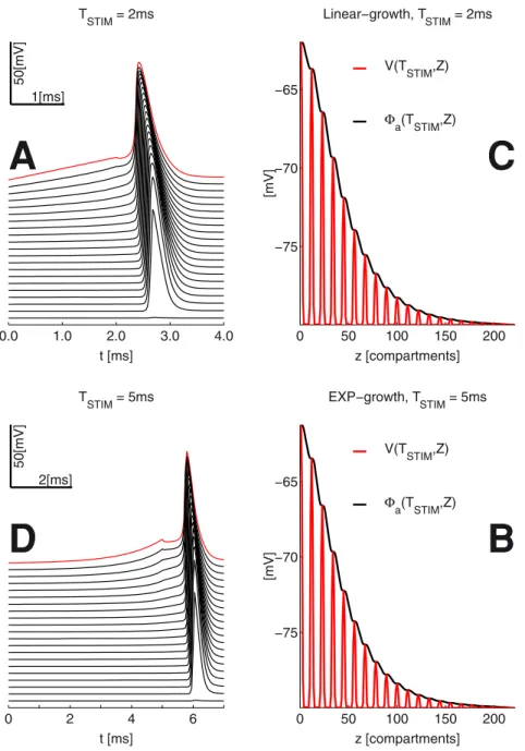
The numerical results presented for the MRG’02 in the literature [7,8] often target the mid-cable (center) RN in their ES simulations. This motivated us to use of the method of mirrors to double the model’s dimensions at the same computational cost. We consider a long axon (with 41 RN’s), which has a relatively low length constant (l2~1=(gara)). See also Tables 4 and 5. For the RN’sl= 167.5mmvs respectively 2129.7 and 443.2mm, for the myelinated and the MYSA (paranode) sections. These are paired to significant differences in the passive membrane time Figure 2. The MRG’02 myelinated axon model (See also Table 4) Box: Equivalent circuit for current injection into the center RN (#1).
constant (t~ci=ga). For the RN’s t= 0.29msvs respectively 20 and 2 ms, for the myelinated and paranode sections. The cable end-conditions are formed by virtual compartments with membrane at restVr=280mV. This choice is further motivated by the results of model simulations - namely the relatively little spread of potentials at the end of stimulation lasting up to a few milliseconds (see Fig. 3).
We studied extensively all the published accounts of the MRG’02 model and its use for ES modeling [7,8,25]. We also carefully compared parameter values (see Tables 5 and 6) to the ones in the official NEURON models database (senselab.med.yale.edu/modeldb/ShowModel.asp?mo-del = 3810).
Our model implementation originally for [29,30] was done in Matlab (the Mathworks, ver. 7 and above). The code uses CVODES (the Lawrence Livermore National Laboratory, Release 2.7.0) to reliably and robustly solve the related multi-dimensional system of ODEs. The implementation was validated through extensive comparisons and personal corre-spondence with the authors of the original model - W.M. Grill [31] and A.G. Richardson, regarding specifically the mismatch between the 2002 publication and its NEURON implementation.
Preliminary Analysis: On the Existence of the AP-firing Threshold
The above ionic-current descriptions differ largely in form and complexity. Yet each of them is capable of capturing some of the essential dynamics properties of excitable living tissues.
In order to elicit an AP through electric stimulation, the membrane’s potentialV(t) needs to first be driven (depolarized,
_ V
Vw0) to some threshold valueVTHR, beyond whichassistingionic channels are massively engaged to produce the AP upstroke without the need of any further ES intervention. From eqn. (6) in order to do so, the stimulation waveform needs to be positive and superior toIS(V,x)at most times - i.e.u(t)needs to overcome the opposingcurrents.
A VTHR value is hiding inside each of the above nonlinear flavors ofIS(V,x). Predictably, it is easiest to find theVTHRvalue associated with the IM. Above we saw that the variablewin the IM reactsslowlyto changes inV. Hence, one may approximate it by its value at rest:wr~bVr. Therestingmembrane potentialVris then obtained from the condition Iion,0(Vr)~0, where the subscript0indicates that we have assumedw(t)~wr.
Theresting potentialVris one of the zeroes of the 2nd-order polynomial in V(t), which characterizes the ionic current. The second zero isVTHR. Beyond this threshold the total ionic current
Table 5.MRG’02 double-cable model-axon electrical parameters.
Notation Parameter description Value
Shared parameters:
Vrest Resting potential 280mV
ra Axoplasmic resistivity 70V
rp Periaxonal resistivity 70V
Nodal compartments:
cn Membrane capacitance 2mF=cm2
EK Kz
Nernst potential 290mV
ENa NazNernst potential 50.0
mV
ELeak Leak reversal potential 290mV
gK,s Maximum slowKzconductance with openingsandnoclosing gate states 0.08S=cm2
gNa,f Maximum fastNazconductance with openingmand closinghgate states 3.0S=cm2
gNa,p Maximum persistentNazconductance with openingpandnoclosing gate states 0.01S=cm2
gLeak Leak conductance 0.007S=cm2
Internodal compartments:
ci Membrane capacitance 2mF=cm2
EPsv Passive-compartment Nernst potential
Passive (leak) membrane conductance by segment type:
ga MYSA 0.001S=cm2
gf FLUT 0.0001S=cm2
gi STIN 0.0001S=cm2
Myelin parameters:
cmy Capacitance 0.1mF=cm2
gmy Conductance 0.001S=cm2
Notes: See also Table 6.
switches its sign. So eqn. (11) becomes:
IION,0(V)~{0:04V2{5VzbVr{140
~{0:04(V{Vr)(V{VTHR)
ð14Þ
Hence,Vr=270 mV and therestingthreshold isVTHR,0=2 55 mV.
We will utilize this simple nonlinear model to complete the picture. Ifw(V,t)wwr- i.e. the membrane isnotat rest, the point where the total ionic current IION(V) switches sign is shifted rightward toward ahigherVTHRvalue. For example, for very long durationsT??,w?bV:
Iion,?(V)~{0:04V2z(b{5)V{140
~{0:04(V{Vr)(V{VTHR)
ð15Þ
The subscript?indicates that we have assumedw(t)~bV(t). Predictably, this does not affect the resting potential, since
Iion,?(Vr)~Iion,0(Vr). However, VTHR,?=250 mV is higher than the resting thresholdVTHR,0.
This reflects the lowering of excitability shortly after an AP, and once the post-AP membrane re-polarization takes place. This is known asrefractoriness, which can be eitherabsolute- i.e. no AP can be elicitedregardlessof how large the stimulation, orrelative -i.e. larger stimulation current is required - to reach a higher thresholdVTHR.
Some models of the HH-type have even more complex
IION,?(V)and thenceVTHRbehavior. This complexity is due to the multiple gate states, which may have very different time constants and hence reach their asymptotic states at different times. In addition, the HH models involve inactivating sodium (Naz
) channels. Hence, excitability may be conditional on attaining the firing threshold within aspecifictime window. Then
VTHR may exist only with durations %?. Hence, even over arbitrarily long duration, an arbitrarily low (non-zero) current may never elicit AP’s, and may also damage the tissues and the electrodes as irreversible chemical reactions take place.
So, wide stimulation pulses lasting well over some critical durationTCRmay not be able to elicit any AP. This is due to the comparable temporal scales of duration TSTIM and the time constanttionof the closing gates associated with depolarizing ionic currents and of the opening gates associated with re-polarizing currents.
Therefore, let us assume that the excitable-membrane’s potential is at its resting valueVr. Hence, in principlean action potential (AP) can be elicited by stimulation of thefixedduration
TvTCR. Therefore stimulation takes place over a finite time-horizon.
Finite-Horizon Optimal-Control (FHOC)
In this approach, the current waveform is the unknown system input signal complying with specific optimality criteria. The optimal pattern u(t) for t[½0,Tis sought as a solution of the
following constrained minimization problem:
u~arg min H(X(T))z ðT
t~0
f0(X,u)dt
ð16Þ
d
dtX~F(X,u) Vu(t)[½L,R
whereLandRare the constant lower and upper bounds on the values for eachu(t)sought.
The computational model’s dynamical system is introduced in the optimization problem of eqn. (16) in the form of a set of equality constraints. ThevectorfunctionF(x,u)[Rndescribes the
dynamics of the array of system state-variable trajectories
xi(t),i~1. . .n, resulting from given initial stateX(0)and control signalu.
The example developed in the Results section uses the Izhikevich model - eqns. (6) and (11) - withn~2.
The minimized functional, contains the integration termf0(X,u)
and a final-time (also known as penalty) termH(X(T))- pulling
toward the desired final state X(T). The specific f0 expression
yields minimum electric stimulation power:
f0(X,u)~u(t)2=2 ð17Þ
The penalty term is a convenient way to express the desirable stimulation’s outcome - the membrane voltage reaching some pre-defined threshold-levelVTHR:
H(x(T))~ Kpenalty
2ðVTHR{V(T)Þ2
ð18Þ
Using a general constrained parametric optimal-control ap-proach (e.g. [32]), the objective and equality constraints in eqn. (16) are combined into theLagrangian:
L~H(x(T))z ðT
t~0
f0(X,u)dt{ 0(d
dtX{F(X,u))
dt
~H(x(T))z½ 0XT
t~0z
ðT
t~0 Hzd
dt 0X
dt
ð19Þ
where (t)are theLagrange multipliers, associated toeachof the
n equality constraints in eqn. (16) and (:)0 stands for the vector-matrixtransposeoperator.H~f0(x,u)z 0F(X,u)is known
as theHamiltonian.
The necessary conditionsfor optimality require that all partial derivatives of the Lagrangian by the system states vanish at the optimal solution to the problem of eqn. (16) - i.e.:
LL
LX(t)~0 Vt[½0,T ð20Þ
Here the ‘vector-matrix’ notations Lw=LX or LF=LX, where X[Rn, mean respectivelyLw=LxiorLfi=Lxj,Vi,j~1. . .n.
This development is known as mathematicalsensitivity analysis and its main purpose is to reveal the impact of a given system parameter (such asu(t) or its initial stateX(0)) on the resulting
dynamics.
From eqns. (19) and (20):
d dt ~{
LH
LX ð21Þ
(T)~
LH
LX(T)
where
LH
LX~
Lf0
LXz
LF
Notice that eqn. (21) describes the adjoint dynamic system iterated inreversetime with aterminalcondition provided by the derivative of theh(X(T))term. To solve the ODE system of eqn.
(21), the achieved forward dynamics of eqn. (16) needs to be already computed.
Similarly, all partial derivatives of the Lagrangian by
u(t),Vt[½0,T vanish at the optimal solution to the problem of
eqn. (16) - i.e.Vk~0. . .m{1:
LL
Luk~
ðT
t~kDt LH
Ludt ð22Þ
whereDtis the sampling time,uk~u(kDt)and
LH
Lu~ Lf0
Luz LF
Lu 0
Hence, eqn. (22) yields all components of the gradient w.r.t.
u(kDt), which enables the use of gradient-based quasi-Newton search routines (e.g. fmincon from the Matlab optimization toolbox).
Moreover, one sees from eqn. (19) that the array (0) is the sensitivity (i.e. the gradient) w.r.t. initial stateX(0), i.e.:
Figure 3. Propagating AP’s and spatial profile of the membrane voltageV(t,z)& intracellular potentialWa(TSTIM,z)(at the end of stimulation, please also see Fig. 2);zis the 1D axonal spatial coordinate.The peaks ofVat the Ranvier nodes are due to the direct exposure to the extracellular medium, which is unlike that of the myelinated sections in the double-cable MRG’02 model.
(0)~
LL
LX(0)
A boundary-value problem (BVP), with knowninitialconditions forX(0)andterminalconditions forl(T), is solved numerically.
However, it should also be noted that such solutions may also converge to shallow local minima. For example, the Newton search is guaranteed to produce the ‘true’ solution when the problem at hand involves a quadratic cost. Here the objective function not only may be quadratic, but also may be non-convex in some manifolds of its high-dimensional parametric space.
Above we described the continuous-time FHOC. The CVODES toolbox readily provides adjoint sensitivity analysis (ASA) capabilities. FHOC is one of the common applications of the latter. Analogously, adiscrete-timeversion may be formulated and solved (see the Results section, where a specific example is developed).
Solving the Problem Analytically: The PLA in ES
Through calculus of variations, here we establish a general form for the energy-optimal current waveform u(t). This approach applies the Principle of Least Action to ES.
Let us assume thatT%tION, wheretION is the time-constant that determines the behavior of theslowgate states of the modeled ionic-channels. Hence, thefastgate states may be approximated by their asymptotic valuesx?(V)~limt??x(tjV), while theslow gate states - by their resting valuesx0~x?(Vr).
Then an AP can readily be evoked by stimulation from the resting state, and the threshold potentialVTHRto reach at timeT
is finite and assumed (without loss of generality) to be known. The energy-efficiency of driving the excitable-tissue membrane poten-tialV(t)from its resting valueVrtoVTHRthrough a stimulation of fixeddurationT satisfies:
u(t)~arg min
u P(u) P(u)~1=2 ðT
0 u(t)
½ 2dt ð23Þ
Since from eqn. (6),u(t)~CmVV_zIS(V):
P(u)~S(VjT,u)~1=2
ðT
0
CmVV_(t)zIS(V)
2
dt ð24Þ
As done in the calculus of variations let us perturb the energy-optimal time-courseV(t)by the infinitesimal perturbationEg(t),
whereg(t)is an arbitrary function of time andEis an infinitesimal
scalar.
V(t)~V(t)zg(t)
IS(V)~IS(V)z
LIS(V)
LV g(t)
ð25Þ
Table 6.MRG’02 double-cable model-axon geometric parameters, inmm.
Notation Parameter description Value
Shared parameters:
D Fiber Diameter 16.0
DZ Node-node separation 1500
Nmy Number of myelin lamellae 150
Nodal compartments:
Ln Node length 1.0
dn Node diameter 5.5
MYSA (myelin attachment paranode)
LM length 3.0
dM diameter 5.5
dM periaxonal width (Membrane-to-Myelin gap) 0.004
FLUT compartments (main section of paranode)
LF length 60.0
dF diameter 12.7
dF periaxonal width 0.004
STIN compartments (internodal section, 3+3 total in 1 internode, see Fig. 2)
LS length 228.8(*1
dS diameter 12.7
dS periaxonal width 0.004
Notes:
(*1LS~DZ{Ln{2(LMzLF)
6 :
From eqn. (25),Vt[½0,Tthe integrand in eqn. (24) becomes:
(CmVV_zIS(V))2~(CmVV_
zIS(V))2
z2 (CmVV_
zIS(V))(Cmgg_zgI’S(V))
z2(Cmgg_zgI’S(V))2
ð26Þ
From eqns. (24) and (26), and sinceu(t)~CmVV_zIS(V).
P( )~S(V)z ðT
0
u(t)(Cmgg_zgIS(0 V))dt
z2F(V,g)
ð27Þ
The necessary condition forS(V)to have aminimumatE~0
foranyg(t)is:
GE~P0( )j~0~
ðT
0
u(t)(Cmgg_zgIS(0 V))dt~0 ð28Þ
To deal with theu(t)gg_term of eqn. (28), it is integrated by parts :
GE~Cm½u(t)g(t)T0{
ðT
0
½Cmuu_{uIS(0 V)g(t)dt~0 ð29Þ
Since the perturbation g(t) respects the boundary-value problem (BVP) with known initial and terminal conditions for
V(t) - i.e. g(0)~g(T)~0, then the first RHS term above vanishes. Hence, the only way that eqn. (29) will hold foranyg(t)
is that we have the Euler-Lagrange-type equation:
Cmuu_~IS(0 V)u ð30Þ
Equation (30) can also be attained directly using the continuous version of the standard OC formalism [32] (please see also the just presented FHOC subsection above).
Here theHamiltonianis.
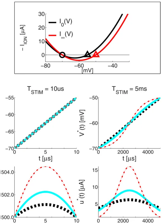
H~u2=2z (u{IS(V))=Cm: ð31Þ Figure 4. LAP energy-optimalV(t)andu(t)for the LM: forT
STIMrespectively 10msand 5ms; the time constantt~C=gwas varied as indicated in the legend; membrane capacity was constant -C= 1mF=cm2, while membrane (leak) conductancegwas respectively 0.2, 1 and 5mS=cm2; The 3 solutions shown correspond to the nominalt= 1ms(cyan trace) or 5-fold shorter (thin red dash-dot), or 5-fold longer (thick dashed black)trespectively; (thin dashed black) rectangular pulse with amplitudek~(VTHR{Vr)=TSTIM.
Thenecessary conditionsfor optimality require that.
LH=Lu~0 ð32Þ
_~{LH=LV ð33Þ
From eqns. (32) and (31) =Cm~{u. Then from eqn. (33). Figure 5. LAP optimal waveformsV(t)andu(t)for the 0D IM: The 3 solutions shown correspond to the nominal IM opposing current (cyan trace), twice higher (thin red dash-dot), or twice lower (thick dashed black)ISrespectively.TheIION,0(V)approximation of the ionic current is used for a case of very short duration (TSTIM= 10ms) and theIION,?(V)approximation is used for a case of long duration
(TSTIM= 5ms). It is important to notice that - as with theLMmodel above,u(t)&kzIION(V), wherek~(VTHR{Vr)=T(see the Box)Box:
Resting-stateIION,0(V)and asymptotic-stateIION,?(V)ionic currents for the 0D IM; Markers are inserted at the resting and threshold
Cmuu_~LH=LV~{ =CmIS(0 V)~uIS0(V)
which is the same as eqn. (30).
From eqns. (6) and (30) we have that.
_ u
u(t)~CmVV€zIS(0 V)VV_~
IS(0 V)u=Cm
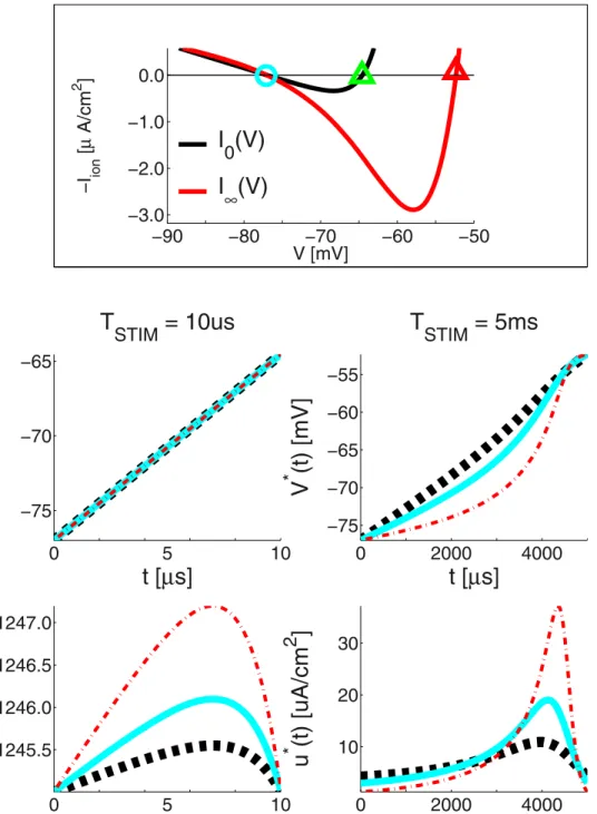
and thence: Figure 6. LAP optimal waveformsV(t)andu(t)for the 0D HHM: TheI
ION,0(V)approximation of the ionic current is used for a case
of very short duration (TSTIM= 10ms) and theIION,?(V)approximation is used for a case of long duration (TSTIM= 5ms) (see the Box).
As with the IM, bvp4c was used to numerically solve the BVP of eqn. (34). The figure follows a quite similar format to Fig. 5.IS(V)can also be
assumed higher or lower. All the maximal ionic conductances in the HHM (see also Table 3) are temperature-dependent and are linearly proportional to the coefficientkT. The 3 solutions shown correspond to the ionic current atToC½37oC(cyan trace), twice higher (thin red dash-dot), or twice
lower (thick dashed black)ISrespectively. From eqn. (42) we can see thatkT= 1.6047 (half the nominal) at28:70C, andkT= 6.4188 (twice the
nominal) for at45:30C.Box:Resting-stateI
ION,0(V)and asymptotic-stateIION,?(V)ionic currents for the 0D HHM; Markers are inserted at the
C2
mVV€
~IS(0 V)½u{C
mVV_:
And finally, from eqn. (6).
C2
mVV€
~IS(V)|LIS(V)
LV ð34Þ
Equation (34) is a rather simple system of ordinary differential equations (ODE) that can readilybe solved for a given current modelIS(V)to compute the energy-optimal membrane voltage
profileV(t). The energy-efficient current waveformu(t)is then
computed from eqn. (6).
In the Results section below we illustrate the use of eqn. (34) with several frequently encountered current models.
Results
Here, we first derive some key analytical results using the simplest and clearest models. We then identify generally applicable optimality principles. Finally, we demonstrate how these principles apply also to more complex and realistic models and their simulations.
Part I - Specific Point-model Results, Applying the LAP For the zero-dimensional (single-compartment, space clamp) models introduced in the Methods, here we describe the LAP-optimal waveformsV(t)andu(t), stemming from the general
(model-independent) LAP result of eqn. (34).
These simple cases readily illustrate some rather key optimality principles resulting from a LAP perspective. We will discuss these optimality principles as we go, and will summarize them at the end of this subsection.
Linear sub-threshold model. ReplacingIS(V)in eqn. (34)
withIION(V)from eqn. (8):
t2VV€~V ð35Þ
t~Cm=gm~RmCm is the membrane’s time constant and for expediencyV:VandVr= 0.
The general solution of eqn. (35) is:
V(t)~C1e {t
tzC2e
t
t ð36Þ
Given the boundary conditionsV(0)~0andV(T)~VTHR:
V(t)~VTHR
sinh (t=t)
sinh (T=t) ð37Þ
A result similar to eqn. (37) is obtained by [33], using a slightly different (less direct or general) optimal-control approach.
From eqn. (37) one can see that V(t)=V
THR~
sinh (t=t)=sinh (T=t)~t=T - i.e. it has a linear rise, especially withT%t. HereT= 100msandt= 1ms(computed usingtypical values from the literature for gm= 1 mS=cm2 and Cm= 1 mF=cm2).
Figure 4 presents the LAP energy-optimal stimulation profiles
V(t) and u(t)for a short and a long stimulus duration TSTIM and three membrane time constanttvalues.
Before we go on, it is useful to investigate the conditions for a growing exponent (GE) waveform to outperform the SQR
waveform. First,u
GE(t)has a very rapid rise. Hence, its optimal duration T
GE will be short. Second, it is noteworthy that in [33]t= 30.4 micro-seconds! Hence, injected current rapidly leaks out. However even with the above extremetvalue, at its optimal durationTSQR theSQRwave does just 22% worse, which means that theSQRis among the best candidates for its robustly good performance.
Second, in multiple cases, the energy-optimal LAP waveform
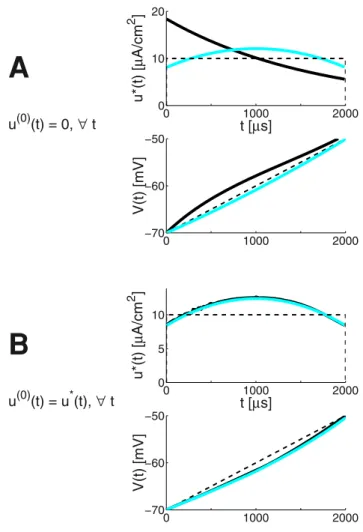
u(t)looks a lot like a ‘classical’ rectangular waveform. From eqn. (8), we may also see that, withVr= 0,VTHR= 1, the max. value of IION(V)is equal to 1 and is attained as the membrane potential reaches the threshold V(T)~VTHR. If we then replace Figure 7. The LAP vs or with numerical optimisation for the 0D
IM, withTSTIM= 2ms: see also Fig. 5 which shows that an initial g u e s s ^uu(t), b a s e d o n t h e l i n e a r- g r o w t h r a t e
k~(V
THR{Vr)=TSTIM is still valid with TSTIM= 2 ms and
VTHR=250 mV. panel A: discrete-time IM and FHOC panel B:
continuous-timeIM and FHOC, using CVODES adjoint sensitivity analysis capabilities upper plots: (dashed black) a rectangular pulse with amplitudek; (thick cyan) the LAP^uu(t)~kzI
ION,?(V); (thick black)
the best FHOCu(t)lower plots:(dashed black)linear-growth evolution of the membrane potential from Vr at t~0 toVTHR at t~TSTIM;
(dotted gray) the desired threshold valueVTHR=250 mV; (thick cyan) the resulting LAPV(t); (thick black) the resulting FHOCV(t).
IION(V)&0in eqn. (6), we see that a waveformu(t)- that brings V(t) from Vr to VTHR at a constant rate, is the time-constant waveform u(t)~k~(VTHR{Vr)=T. For this example, k~
10&IION(V), which explains why u(t) is that close to a rectangular waveform.
As a matter of fact, for very short stimulation times, thektend
to be high, whileIION(V)tends to be linear. Hence, the ‘classic’ rectangular (or square,SQR) waveform tends to also be close to energy-optimal.
Such facts are rather important as they lead us below (as evidence is accumulated) to a general form not only ofV(t), but
also ofu(t).
Comparative properties theV(t) growth profiles. The
GE waveform may be anSQRwaveform in disguise. I.e. some
linear growth of the membrane voltage may still fit the one obtained upon ES with aGE. The motivation for this is in eqn. (36), where the first term vanishes withT&t.
Finally, the total electric charge conveyed by the ES source may have to be considered. For example, in theLMof eqn. (8) the total charge consists of a capacitive charge to raise the membrane voltage by a given amount (to VTHR), and resistive charge ÐTSTIM
0 V(t)=Rdt. A similar situation occurs in theMRG002model
due to the opposing axial currents.
So let us solve the following auxiliary problem:
Find a linear fitVV^(t)~max½a(t{b),0to the growing exponent
V(t)~(et=t{1)=(eTSTIM=t{1), so that the ES source conveys the same resistive charge in the time intervalt[½0,TSTIM. I.e. we want
that:
ðTSTIM
0 ^ V V(t)dt~
ðTSTIM
0
V(t)dt~t{ TSTIM
eTSTIM=t{1
Here, for simplicity (and without any loss of generality) we have assumedVr~0andVTHR~1.
For example witht~TSTIM=4, we obtainb&0:54|TSTIM, i.e. the linear-growth equivalent has more than twice shorter duration - e.g. withTSTIM~5,b&2:7.
The latter result promotes intuition: with large opposing currents optimal ES cannotaffordto last long. The transition of the membrane voltage from its rest to a threshold value is best performed rapidly. Hence, the shape of theV(t) growth profile depend on theTSTIM=tratio. As seen, forTSTIM%t, the optimal u(t) is close to rectangular, while withTSTIM&t, the GE is in effect equivalent to doing nothing for at least half of the duration, and then to aSQRwaveform of at least doubled amplitude.
With quite similar reasoning, one can demonstrate that a 1st-order membrane voltage growth profile V(t)~(1{et=t)= (1{eTSTIM=t) in the time intervalt[½0,TSTIMis suboptimal and
equivalent to linear growth, which has about twice longer duration.
Izhikevich model. ReplacingIS(V) in eqn. (34) with the
IION(V)approximations from eqn. (14) or (15), see Box in Fig. 5:
Cm2VV€~0:042(V{Vr)(V{VTHR)½2V{(VrzVTHR) ð38Þ
As in the preceding modelV:V. Note that the dynamics of
eqn. (38) has all FP’s of IION(V), as well as a third FP at V~0:5(VrzVTHR), contributed by the derivative termIION0 (V). Equation (38) can be solved analytically. However, it provides the solution in an implicit form and involves an incomplete elliptic integral of the first kind. Hence, we used the Matlab bvp4c BVP solver with boundary conditions V(0)~Vr and V(TSTIM)~ VTHR.
Figure 5 illustrates the energy-optimal LAP solutionu(t) and
the corresponding membrane voltage profileV(t). TheI
ION,0(V) approximation of the ionic current is used for a case of very short duration (TSTIM= 10 ms) and the IION,?(V) approximation is used for a case of long duration (TSTIM= 5ms).
It is important to notice that - as with the LM model above,
u(t)&kzI
ION(V), wherek~(VTHR{Vr)=T (see the Box in Fig. 5).
According to eqns. (14) and (15) the opposing current in the IM can be presented in the general form:
Figure 8. The MRG’02 model: Toward upper bounds on
VTHR(TSTIM): the figure presents a family of ionic current
IION(V,Z)approximations at the target site (Z~0), for a set of durations TSTIM. For each of the durations it is assumed that the
membrane voltage trajectoryV(t)evolves according to a linear ramp from restVrto thresholdVTHR(the unknown). For eachVvalue on the
horizontal (independent-variable) axis of the figure, aV(t)~ktramp was assumed and the corresponding ionic current IION(V) was
computed, based on approximate gate states (see the Box). Note: for the sake of better visibility, a |10 gain is applied to the approx. IION(V)for the case ofTSTIM= 5ms.Box:For a chosenTSTIM= 5ms
and asV(t)is linearly ramped up, for each gate state the plots show the ratio^xx(V,T)=x?(V), wherexx^is given by eqn. (46) to its asymptotic
value - both functions ofV. Legend for gate states: openingm and closinghgates for thefastNaz
ion-channel subtype;ppersistentNaz
channel gates;sslowKz
IS(V)~gain|^IIION(V) ð39Þ
where the nominal gain= 1, and ^IIION(V)~0:04(V{Vr)
(V{VTHR).
To see how the optimal ES is affected by the level of opposing current, it is more than tempting to experiment with differentgain
values.
Hence, 3gaincases are plotted in Fig. 5 - for the nominalgain
(cyan traces) and two additional cases: the opposing current
IS(V) is either doubled (gain= 2, red traces) or decreased two-fold (gain= 1/2, black traces). As could be intuitively expected
from the general equation (24), whenIION(V)?0(very low ionic currents):
ðTSTIM
0
u2dt*
ðTSTIM
0 _ V
V2dt ð40Þ
By theCauchy-Schwartz inequality in the space of continuous real functions, it is straightforward to show that the voltage trajectoryV(t)that minimizes eqn. (40) is such that VV_(t)~k,
wherekis determined from the boundary conditions satisfied by V(t). Hence:
Figure 9. The actually computedV
THR as a function ofTSTIM : Notice how the computedVTHR value is rather similar (almost matched) between the linear and exponential cases, forTSTIMrespectively 2 and 5 ms; and between the1st-order and linear cases, forTSTIMrespectively 0.2 and 0.5 ms. see also Fig. 10.
doi:10.1371/journal.pone.0090480.g009
Table 7.MinimalVTHR(TSTIM)½mVvalues for the MRG’02 model, obtained for eachV(t)trajectory class.
TSTIM Linear 1st-order Exponent.
0.020 225.649 237.602 24.963
0.050 241.838 250.515 224.311
0.100 250.852 257.366 237.032
0.200 257.061 261.506 247.137
0.400 260.588 263.558 254.124
0.500 261.247 263.889 255.731
1.000 262.378 263.960 259.255
2.000 261.950 262.578 260.977
5.000 259.273 259.094 261.249
k~VTHR{Vr
TSTIM
ð41Þ
Just as in the preceding model, it is alsoV(t)=V
THR~t=TSTIM with the shorter durations - which justifies the use of the resting approximationIION,0(V).
HHM. Here the IS(V) of eqn. (34) is replaced with the
resting-state - IION,0(V), or asymptotic-state - IION,?(V) ionic current approximations (see the Box in Fig. 6).
TowardIION,0(V) the gate-state variables are factored out as follows: The fast state m(t)&m?(V), while the slower variables h(t)&hr~h?(Vr), and n(t)&nr~n?(Vr) are approximately at rest, assuming very short durations. Conversely, and assuming very long durations, toward IION,?(V) all gate variables are approximately at their asymptotic value, corresponding to a given membrane voltageV(t)(see Methods).
As with the IM, we used bvp4c to numerically solve the BVP of eqn. (34) with boundary conditionsV(0)~V
randV(TSTIM)~ VTHR.
Figure 6 follows a very similar format to Fig. 5.
Similarly to eqn. (39) above,IS(V)can also be assumed higher
or lower. All the maximal ionic conductances in the HHM (see also Table 3) are temperature-dependent and are linearly proportional to the coefficientkT:
kT~Q
(T{T0)=10
10 ð42Þ
whereQ10~2:3andT0= 23uC. Hence withT= 37uC, according
to eqn. (42)kT= 3.2094. Let this be ourstandardcase (gain= 1). As we did with the IM, 3 gain cases are plotted in Fig. 6 for
IS(V)~gain|^II
ION(V). For the two additional cases the opposing current IS(V) is either doubled (gain= 2, red traces)
or halved (gain= 1/2, black traces).
Once again - as with the LM and IM models above,
u(t)&kzI
ION(V)(see the Box in Fig. 6).
Numerical model simulation and optimal control. The
IM was also evoked in the FHOC Methods section. It is therefore interesting to contrast the results of the LAP and FHOC approaches in identifying energy-optimal ES waveforms for the same ionic current model. For such comparison, the IM has the clear advantage of hiding no implementation specifics inside a black box.
The FHOC formalism (see Methods) is computationally efficient, but it is also subject to the similar limitations as most of the ad-hoc search approaches. Iterative numerical optimization requires an initial guess for the solution, and trying different starting arraysu(0)may alleviate a bit the propensity to converge to
shallow local energy-minima.
Here it is also important to realize that in eqn. (16) the two terms to minimize in theF(u)functional (a function of functions), namely the energy cost (17) and the penalty (18) may conflict each other. When the penalty gainKpenaltyin (18) is too low, the search will identify a lower-energy solutionu, which however does not bring the membrane potentialVkup to the desired threshold value - i.e.VM%VTHR. Conversely, a too high penalty gainKpenaltywill identify a very high-energy solutionu, which is not only costly, but the membrane potential may also overshoot the threshold, since Figure 10. The energyPand charge-transferQvalues as a function ofTSTIM : The linear-ramp voltage profile yields the bestP performance for most of the durations.As in Fig. 8 notice that thePandQvalues are quite similar for the linear and exponential cases, for TSTIM respectively 2 and 5 ms; and also for the1st-order and linear cases, forTSTIM respectively 0.2 and 0.5 ms. Toward thePvalues electrode
the ‘getting there’ is underestimated for the sake of the very last simulation steps.
As seen from Fig. 7 Panel B (which uses the IION,?(V) approximation of the ionic current for the relatively long duration
TSTIM= 2ms), the linear growth profile is a reasonable estimate for the optimal membrane voltage profileV(t). Hence:
u(t)&kzI
ION,?(V) ð43Þ
where k is given by eqn. (41). When u(0) is close to the LAP
estimateu(t) of eqn. (43), the FHOC iteration also consistently ends close to there (see Fig. 7, panel B). The cyan traces on Fig. 7 are theu(t)and the resultingV(t). With the LAP estimate, the FHOC approach resulted in a final membrane potential reasonably close to the desired threshold value - i.e.
V(TSTIM)~{50:106&VTHR~{50, even if the IM was simu-lated with the discretized LAP waveformu(t)(Dt= 10ms).
The black traces illustrate the FHOC solution, computed for two differentu(0)choices. For Panel A,u(0) was chosen to be all
zeros. When all time-step entriesu(0) were chosen to be equal to
the upper boundU= 30 (data not shown), due to the (discontin-uous) AP event occurring mid-way the temporal horizon, the Matlab’s fmincon solver remains stuck to the initially provided values.
Except for the case in Panel B, theKpenaltymeta-parameter had to be kept high (Kpenalty= 70) in order to respect the terminal constraint ofV(TSTIM)&VTHR.
The total energy costs (all expressed as 2-norms of the obtained bestu(t)) are respectively 161, 153.2 and 423.4 (for the discrete-time version) 186.7, 159.1 and 334.2 (for the continuous-discrete-time version).
Comparing these toP(u)= 153.2 (discrete-time) and = 157.4 (continuous-time), the LAP-based solution is comparable to or superior than the FHOC solutions. The numerical FHOC solution on Fig. 7, panel A has converged to a local extremum. Note that a post-hoc correction (simple DC offset) is applied to the LAP-based estimate, which adjusts for the overshoot ofVTHRwhen simulating the full (two-dimensional) IM. The overshoot is due to using the one-dimensional approximation, eqn. (15).
The results obtained here nicely illustrate multiple aspects of identifying energy-efficient waveforms through numerical model simulation and optimization. Clearly, pairing theoretical insights with numerical tools carries the best success potential.
Part I Results Summary
A number of more general observations onu(t)can be made
looking at the results this far.
Probably, the most significant result is that the use of LAP reduces the problem to the BVP, defined by eqn. (34), with
V(0)~V
randV(TSTIM)~VTHR. We still need to have a very good idea of bothIS(V)andVTHRto successfully solve forV(t), and thence foru(t), in a given particular situation.
We identify also the following key and practice-oriented optimality principles resulting from the LAP perspective.
1. The optimal sub-threshold membrane potential growth profile with relatively short durations TSTIM and low membrane conductivity:
First, in all simple models we used up to here, the solutionV(t)
of the ODE system, defined by eqn. (34), is quite close to a linear growth fromV(0)~V
rtoV(TSTIM)~VTHR. Second, with the total currentIS(V)&0(e.g. low leak), then from eqn. (6), it follows thatu(t)will be exactly proportional to the rate of change of the membrane’s potentialV(t). IfVV_(t)&const, then u(t)is close to aSQRwaveform.
2. The energy-efficient waveform depends directly on the temporal shape of currents at the AP initiation site.
3. The targeted VTHR membrane voltage threshold depends on stimulation duration, with a tendency to increase withTSTIM. 4. The exponential growth membrane voltage profiles V(t) are
equivalent to linear growths of shorter duration.
Part II - Multiple-compartment Model Results
Here we first extend the general (model-independent) LAP result of eqn. (34) to spatial-structure models (non-zero-dimen-sional, multi-compartment), which involve membrane-voltage distribution and propagation along cable structures.
LAP result generalization to multi-compartment
models. There is a combinatorial explosion in both the number
of parameters and the number of ways that multi-compartment models can be put together and used. Hence, there is much more than one way of generalizing the LAP result of eqn. (34).
Here we briefly present a variant, which appears to be one of the most straightforward generalizations.
Table 8.MinimalQ(TSTIM)½pico{Coulombvalues for the MRG’02 model, obtained for eachV(t)trajectory class.
TSTIM SQR Linear 1st-order Exponent.
0.0200 3.1180 0.1279 0.1671 0.1467
0.0500 1.2472 0.1630 0.1946 0.1642
0.1000 0.6236 0.1959 0.2212 0.1847
0.2000 0.3832 0.2369 0.2583 0.2121
0.4000 0.3426 0.3045 0.3191 0.2545
0.5000 0.2605 0.3440 0.3492 0.2937
1.0000 0.2143 0.5093 0.4736 0.3910
2.0000 0.1808 0.8640 0.6361 0.5855
5.0000 0.1411 2.1216 1.5673 1.2018
With a multi-compartment model, eqn. (7) can be rewritten as:
L
LtV(t,Z)~u(t,Z){IS(V,Z) ð44Þ
Without loss of generality, we used the variableZto represent any ‘spatial’ model dimension. It could even stand for the compartment index in a discretized implementation.
Now, eqn. (7) is a partial DE, depending both on the temporal and the spatial model dimensions.
Assuming that we are free to manipulate u(t,Z) in every compartment as we wish, the derivation sequence from eqn. (23) to eqn. (30) (see the LAP subsection in the Methods) still applies yielding a family of equations ‘parameterized’ by the location coordinateZ.
Hence, we may obtain the generalization of eqn. (34) as:
Cm2 L 2
Lt2V
(t,Z)~IS(V,Z)| L LVIS(V
,Z) ð45Þ
Like the extended eqn. (44), eqn. (45) is a partial DE, depending on both temporal and spatial boundary conditions. In particular,
VTHR becomes a function ofZ. It is no longer a single variable, but a whole spatial profile, subject to conditions such as thesafety factorfor propagation introduced in the cardiac literature [34].
The MRG’02 model: Toward upper bounds on
VTHR(TSTIM). Multi-compartment models add complexity unseen with the single-compartment models. Wongsarnpigoon & Grill [8] used the peripheral-axon MRG’02 model [25] in a genetic-programming search for energy-efficient stimulation waveforms. The approach was somewhat similar to the FHOC described above. After thousands of iterations simulating the MRG’02 model, the identified waveforms were reminiscent of noisy truncated and vertically offset Gaussian’s (Fig. 2 in [8]). In the light of analysis this far one might think that this reflects the shape ofIS(V)forVranging from the resting value (280 mV) to some thresholdVTHR.
In this work stimulation is assumed to be intracellular and at just one spatial location (Z~0, the center RN, see Methods) along the cable structure.
To suggest a version of optimal waveforms u(t) for the
MRG’02 model, we first estimate the membrane voltage threshold for each duration. One analytic way toward such estimates is Figure 11. Optimal waveforms u(t), T
STIM= 20, 200 ms: The figure also provides the corresponding optimal SQR-like linear-growth-related current Cm|k (dashed black), as well as the components ofIS- respectively the IION (blue traces) andIaxial(red traces) current trajectories.
doi:10.1371/journal.pone.0090480.g011
Figure 12. Optimal waveformsu(t): see also Fig. 11. Notes:
Since hereVt,VV_(t)~k, wherekis given by eqn. (41), from eqn. (6)
u(t)~C
mkzIS(V). The figure is optimized to present clearly both
u(t)andk(*1)The dashed trace at the bottom plotslog
10Cmkas a
function of TSTIM (*2) Toward equally good plot visibility, for all
durationsTSTIMv1ms, the waveformsu(t)arerubber-bandedto take
the same graph width as the 1 ms-waveform. This is illustrated by the scale bars for the shortest durationTSTIM= 20ms.(*3)The vertical scale
is the same for all plots, except for the logarithmic offset, as defined by pt. (*1) above.