UNIVERSIDADE FEDERAL DO CEARÁ CENTRO DE CIÊNCIAS
DEPARTAMENTO DE FÍSICA
PROGRAMA DE PÓS-GRADUAÇÃO EM FÍSICA
UNIVERSITEIT ANTWERPEN FACULTEIT WETENSCHAPPEN
DEPARTEMENT FYSICA
Jorge Luiz Coelho Domingos
Estudo de sistemas coloidais de partículas anisotrópicas
magnéticas
Study of colloidal systems of anisotropic magnetic particles
Studie van colloïdale systemen van magnetische anisotrope
deeltjes.
Estudo de sistemas coloidais de partículas anisotrópicas
magnéticas
Study of colloidal systems of anisotropic magnetic particles
Studie van colloïdale systemen van magnetische anisotrope
deeltjes.
Tese apresentada ao Curso de Pós-graduação em Física da Universidade Federal do Ceará como parte dos requisitos necessários para a obtenção do título de Doutor em Física.
Orientador:
Prof. Dr. Wandemberg Paiva Ferreira Co-orientador:
Prof. Dr. François M. Peeters
DOUTORADO EM FÍSICA DEPARTAMENTO DE FÍSICA
PROGRAMA DE PÓS-GRADUAÇÃO EM FÍSICA CENTRO DE CIÊNCIAS
UNIVERSIDADE FEDERAL DO CEARÁ
Dados Internacionais de Catalogação na Publicação Universidade Federal do Ceará
Biblioteca Universitária
Gerada automaticamente pelo módulo Catalog, mediante os dados fornecidos pelo(a) autor(a)
C617e Coelho Domingos, Jorge Luiz.
Estudo de sistemas coloidais de partículas anistrópicas magnéticas / Jorge Luiz Coelho Domingos. – 2018. 114 f. : il. color.
Tese (doutorado) – Universidade Federal do Ceará, Centro de Ciências, Programa de Pós-Graduação em Física , Fortaleza, 2018.
Orientação: Prof. Dr. Wandemberg Paiva Ferreira. Coorientação: Prof. Dr. François Maria Leopold Peeters.
1. Matéria mole. 2. Auto-organização. 3. Colóides magnéticos. 4. Percolação. 5. Dinâmica Molecular. I. Título.
STUDY OF COLLOIDAL SYSTEMS OF ANISOTROPIC MAGNETIC PARTICLES
Tese de Doutorado apresentada ao Programa de Pós-Graduação em Física do Departamento de Física da Universidade Federal do Ceará, como requisito parcial para obtenção do título de Doutor em Física. Área de concentração: Física da Matéria Condensada.
Aprovada em: 15/03/2018.
BANCA EXAMINADORA
_________________________________________________ Dr. Wandemberg Paiva Ferreira (Orientador)
Universidade Federal do Ceará (UFC)
_________________________________________ Dr. Gil de Aquino Farias
Universidade Federal do Ceará (UFC)
_________________________________________ Dr. Pierre Basílio Fechine
Universidade Federal do Ceará (UFC)
_________________________________________ Dr. François Maria Leopold Peeters
University Antwerp (Bélgica)
_________________________________________ Dr. Diego Rabêlo da Costa
University of Minnesota (UM)
_________________________________________ Dr. Luciano Rodrigues da Silva
Acknowledgments
To God, parents (Jorge and Cristina) and my wife (Hiatanara), because I owe it all to you for supporting me in my darkest and sadly days, for believing me when I was discredited and for always helping me to keep moving on. A special mention to my aunt (Terezinha) and my cousin (Romero), for all encouragement. You are great! Love you all!!
To my former teacher Luciana Colares (Tia Lulu), whom I express my eternal gratitude for her advices, support and love. Thank you.
To my supervisor, Prof. Dr. Wandemberg, for his guidance, support and friendship since my scientific initiation. I am really grateful. To my co-supervisor, Prof. Dr. François Peeters for all his insightful comments to improve this thesis and for his support during my stay in Belgium. Thank you. I would also like to thank Prof. Dr. Felipe Munarin, for help me a lot in the beginning of my PhD.
I thank the other members of the jury, Prof. Gil de Aquino, Prof. Luciano da Silva, Prof. Pierre Fechine and Dr. Diego Rabelo for the time spent reviewing this work, as well as for their very important comments, corrections and suggestions that made possible to improve the quality of the final version of this thesis.
I am grateful to all my friends for accepting nothing less than excellence for me. All of you, directly or indirectly involved in my thesis, helped me to move forward when the troubles appeared. With a special mention to my GTMC colleagues: Diego Rabelo, Davi Soares,Jorge Bezerra,Danilo Borges,Diego Lucena andLevi, also to my CMT colleagues: Victor, Rebeca and Luca. It is and it has always been a pleasure to share a time with you. For those friends not-involved directly in my thesis, it would be unfair if I forgot any names, so I’ll just keep it simple and plain: Thank you very much for all the support throughout these years.
Da terra querida, que a linda cabocla De riso na boca zomba no sofrer
Não nego meu sangue, não nego meu nome Olho para a fome, pergunto o que há? Eu sou brasileiro, filho do Nordeste, Sou cabra da Peste, sou do Ceará..”
9
Resumo
O processo de auto-organização de um sistema bidimensional de barras magnéticas é estudado. As barras são modeladas como contas dipolares unidas e alinhadas, o chamado modelo vagem. O sistema é estudado por meio das simulações de Dinâmica Molecular e Dinâmica de Langevin. Inicialmente, uma introdução sobre os sistemas de matéria mole, mostrando suas principais características e alguns aspectos teóricos e experimentais é ap-resentada. A seguir, são apresentados e discutidos os métodos computacionais adotados nas simulações, bem como o tratamento matemático do sistema. Quanto aos resultados da tese, uma diversidade de configurações auto-organizadas, tais como: (1) aglomera-dos, (2) percolados e (3) estruturas ordenadas são obtidas e caracterizadas em relação ao estado de agregação das partículas e ordenamento. Ao aumentar a razão de aspecto das barras magnéticas, verifica-se que em duas dimensões a transição de percolação é suprimida. Este resultado é oposto ao que é observado em sistemas semelhantes em três dimensões. Mostra-se que esse comportamento é uma conseqüência de efeitos geométricos que reduzem a mobilidade das barras à medida que a razão de aspecto destas é aumen-tada. No que diz respeito ao ordenamento das partículas no sistema, uma fase magnética é encontrada com ordenamento ferromagnético local, e também é observado um compor-tamento não monotônico incomum da ordem nemática. Com base também em simulações de Dinâmica de Langevin, as configurações auto-organizadas são estudadas para o caso especial em que o dipolo das contas que constituem as barras está desalinhado em relação ao eixo da barra. O desalinhamento é zero quando o dipolo é paralelo ao eixo axial. Verificou-se que a densidade necessária para a formação da estrutura percolada diminui com o aumento do desalinhamento do dipolo. Além disso, o sistema exibe diferentes es-tados de agregação (sólido ou líquido) para diferentes desalinhamentos, mesmo quando a mesma densidade é considerada. A estabilidade das estruturas auto-organizadas é estu-dada em relação à temperatura, e geralmente aumenta com o aumento do desalinhamento dos dipolos.
The self-assembly process of a two-dimensional ensemble of magnetic rods is studied. The rods are modelled as aligned single dipolar beads, the so-called peapod model. The system is studied by means of Molecular Dynamics and Langevin Dynamics simulations. An introduction on soft matter systems, showing their main features and some theoretical and experimental aspects is first presented. In the following, the computational methods adopted in the simulations and the mathematical treatment of the system are presented and discussed. Concerning the results of the thesis, a diversity of self-assembled configu-rations such as: (1) clusters, (2) percolated and (3) ordered structures are obtained and characterized with respect to the state of aggregation of the particles and ordering. By increasing the aspect ratio of the magnetic rods, it is found that in two dimensions the percolation transition is suppressed. This is opposite to what is observed in similar three dimensional systems. It is shown that such a behavior is a consequence of geometrical effects which reduce the mobility of the rods as the aspect ratio of such rods is increased. Concerning the ordering of the particles in the system, a magnetic bulk phase is found with local ferromagnetic order and an unusual non-monotonic behavior of the nematic order is also observed. Based also on extensive Langevin Dynamics simulations, the self-assembled configurations are studied for the special case where the dipole of the beads that constitute the rods are misaligned with respect to the rod axis. The misalignment is zero when the dipole is parallel to the axial axis. It is found that the density required for the formation of the percolated structure decreases with increasing misalignment of the dipole. Also, the system exhibits different aggregation states (solid or liquid) for different misalignment, even when the same density is considered. The stability of the self-assembled structures are studied with respect to temperature, and it usually increases with increasing misalignment of the dipoles.
Abstract
Het zelf-assemblageproces van een tweedimensionaal ensemble van magnetische staven wordt bestudeerd. De staven zijn gemodelleerd als uitgelijnde enkele dipolaire kralen, het zogenaamde peapod-model. Het systeem wordt bestudeerd met behulp van Molec-ulaire Dynamica en Langevin Dynamica-simulaties. Een inleiding over zachte-materie-systemen, waarin hun belangrijkste kenmerken en enkele theoretische en experimentele aspecten worden besnoken. Vewolgens worden de berekeningsmethoden die in de sim-ulaties en de wiskundige behandeling van het systeem zijn gebruikt gepresenteerd en besproken. Met betrekking tot de resultaten van het proefschrift, wordt een diversiteit aan zelf-geassembleerde configuraties zoals: (1) clusters, (2) gepercoleerde en (3) geor-dende structuren verkregen en gekarakteriseerd met betrekking tot aggregatietoestand van de deeltjes en ordening. Door de aspect-verhouding van de magnetische staven te vergroten, vonden we dat in twee dimensies de percolatietransitie wordt onderdrukt. Dit is tegengesteld aan wat wordt waargenomen in vergelijkbare driedimensionale systemen. Er wordt aangetoond dat een dergelijk gedrag een gevolg is van geometrische effecten die de mobiliteit van de staven verminderen, aangezien de aspect-verhouding van dergeli-jke staven toeneemt. Wat betreft de ordening van de deeltjes in het systeem, wordt een magnetische bulkfase gevonden met lokale ferromagnetische orde en een ongewoon niet-monotoon gedrag van de nematische orde wordt ook waargenomen. Gebaseerd op uitgebreide Langevin Dynamica-simulaties, worden de zelf-geassembleerde configuraties bestudeerd voor het speciale geval waarbij de dipool van de korrels die de staven vormen, ten opzichte van de staafas niet goed uitgelijnd is. De foutieve uitlijning is nul wanneer de dipool parallel is aan de axiale as. We vonden dat de dichtheid die vereist is voor de vorming van de gepercoleerde structuur afneemt met toenemende foutieve uitlijning van de dipool. Ook vertoont het systeem verschillende aggregatietoestanden (vast of vloeibaar) voor verschillende scheefstanden, zelfs wanneer dezelfde dichtheid wordt beschouwd. De stabiliteit van de zelf-geassembleerde structuren wordt bestudeerd met betrekking tot temperatuur, en deze neemt gewoonlijk toe met toenemende scheefstand van de dipolen.
List of Figures 14
List of abbreviations 19
List of nomenclatures 20
Part I - Introduction 21
1 Introduction and Overview 23
1.1 Soft Matter systems . . . 23
1.2 Colloidal Dispersion. . . 25
1.2.1 Pair interaction between colloids. . . 26
1.2.2 Magnetic Nanoparticles . . . 29
1.2.3 Magnetic Rods . . . 30
1.3 Liquid Crystals-Like States. . . 33
Part II - Theoretical framework and methodology 36 2 Numerical Methods 38 2.1 Molecular Dynamics Simulation . . . 38
2.1.1 Integration of The Equations of Motion . . . 41
2.1.2 Periodic Boundary Conditions . . . 42
2.1.3 Statistical Mechanics and Molecular Dynamics . . . 44
2.1.4 Molecular Dynamics Scheme . . . 46
2.1.5 Control of Temperature . . . 47
2.1.6 Important Measured Quantities . . . 48
2.2 Langevin Dynamics . . . 52
2.2.1 Langevin Equations for Rod-like particles. . . 53
13
Part III - Results 62
3 Self-assembly of rigid magnetic rods consisting of single dipolar beads
in two dimensions 64
3.1 Motivation . . . 64
3.2 Model . . . 65
3.3 Cluster Formation. . . 68
3.4 Connectivity properties . . . 72
3.5 Orientational Ordering . . . 77
3.6 Conclusions . . . 78
4 Clustering and percolation properties of magnetic peapod-like rods with tunable directional interaction 79 4.1 Introduction . . . 79
4.2 Model and Simulation Methods . . . 81
4.3 Results and Discussion . . . 84
4.3.1 Cluster Formation . . . 84
4.3.2 Connectivity Properties . . . 88
4.3.3 Effect of temperature . . . 93
4.4 Conclusion . . . 94
5 Concluding Remarks 96
Appendix A
Derivation of the torque on a magnetic rod composed by dipolar beads 99 Appendix B
Publications related to this thesis 105
1.1 Examples of soft matter systems. Top panel: (left) polystyrene (polymers), and (right) jelly (colloids). Bottom panel: (left) detergents (surfactants), and (right) LCDs (liquid crystals). . . 23
1.2 Illustrative triangle showing the continuum of molecules and materials which fills the space between spherical colloids, flexible polymers, and sur-factants. Extracted from Ref. [2]. . . 24
1.3 Examples of colloids. (a) Paints. (b) Viruses. (c) Milk. (d) Ferrofluid. (f) Colloidal Crystals. . . 26
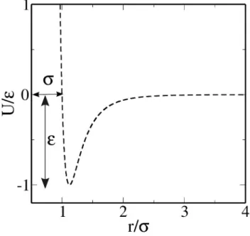
1.4 Lennard-Jones potential curve.. . . 27
1.5 Total DSS pair potential for different configurations as a function of the interparticle separation. For comparison purposes, LJ curve is also plot-ted in the black solid line. A sketch with the relevant parameters in the interaction is also shown. . . 29
1.6 In situ image by Transmission Electron Microscopy (TEM) of dispersion of F e3O4 inC10H18 (a) without magnetic field (b) with homogeneous
mag-netic field (0.2T). The transition occurs for equally spaced column that displays hexagonal symmetry. Figure extracted from Ref. [21]. . . 30
1.7 TEM images of dispersion of magnetic rods. (a) β-FeOOH nanoparticles. (b) Silica-coated β-FeOOH nanoparticles. (c) Iron oxide/silica nanocom-posite after calcination at 500◦ C for 5h. Figure extracted from Ref.
[32].(d)-(e)-(f) TEM micrographs of the nanorods (45 to 450 nm). Fig-ure extracted from Ref. [35]. . . 31
1.8 Two possible approaches to simulate nanorods: (a) MNR approach, where each particle has a diameter σ and dipole moment m, the lenght of each rod islσ. (b) Spheroids with dipole momentme for minor radius band the
15
1.9 Schematic representation of the experimental rods synthesis procedure. (a) The magnetic dipole moment (white arrows) are aligned to an external field
H0during deposition. (b) Magnetic field assisted self-assembly of individual
dipolar rods. The build-up of field gradients is symbolized by flux-lines. (c) Further growth of individual rods is accompanied by a change in growth mode resulting in the formation of bundles of rods. Figure extracted from Ref. [37].. . . 32
1.10 Peanut-shaped particles with a permanent transverse magnetic dipole. Fig-ure extracted from Ref. [39]. . . 33
1.11 Illustration of a formation of ribbon-like chains by magnetic rods with a non-axial dipole moment. Figure extracted from Ref. [40]. . . 33
1.12 Examples of Liquid crystals. . . 34
2.1 Illustration of important parameters of a linear rigid body model. . . 40
2.2 Illustration of a 2D system subject to PBC. The yellow-shaded box repre-sents the central (real) simulation box. . . 44
2.3 Some examples of classic phase spaces - (a) Phase space of a free particle for 0< x < L and p, p+δp - (b) Phase space for harmonic oscillator with
energy E, E+δE . . . 45
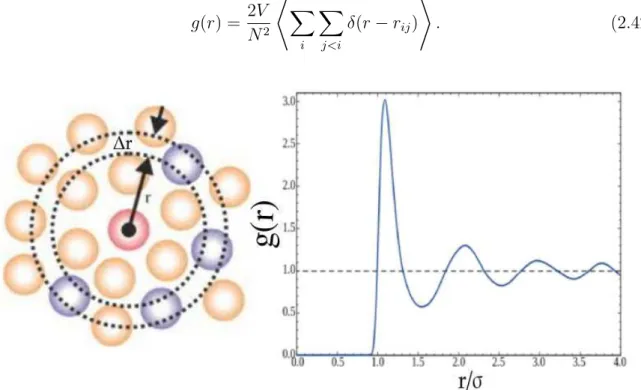
2.4 Illustration of evaluation of the pair correlation function. (a) In the center there is a reference particle (pink circle). The spheres around represent other particles in the system. A centered ring is drawn as reference and it has radius r, relative to the reference particle, and width ∆r. (b) As an
example, we show the typical radial distribution function for a LJ system in the liquid phase. Modified from Refs. [56, 57]. . . 48
2.5 (a) Cluster size distribution for packing fractionη = 0.01(ratio of the
occu-pied area over the available area) at several temperatures; (b) Cluster size distribution close to percolation (T = 0.078and density ρ= 0.1). To
mini-mize size effects,40000particles have been simulated. The different straight
lines show the theoretical predictions for mean-field and 2d-percolation, as well as the best fitting slope of the numerical cluster distribution. The cluster size predicted by the Flory–Stockmayer (FS) theory [60] is also re-ported, but its range of validity is limited to only small clusters. ρ(s)stands
for the frequency of appearance of s-sized cluster. Extracted from Ref. [61]. 50
2.6 (a) Percolation probability as a function of the volume fraction for different aspect ratio (l) and dipole moment (m). (b) Example of a 3D-percolated
2.7 Cluster size distribution for a short range attraction and long range repul-sion system showing four possibles states. The dispersed fluid is mainly represented by monomers. However, for systems when there are clusters with small or medium size we have the clustered fluid. And for the perco-lated phases, in the percolation threshold theN(s)will exhibit a power-law
decay with a specific critical exponent related to the random percolation prediction, but the cluster percolated phase is a distinctly different struc-tural state due to a different concentration and a preferred cluster size. Extracted from Ref. [63]. . . 52
2.8 The peapod-like rod representation and the definition of the vector R on
the surface of a bead. Modified from Ref. [73]. . . 55
2.9 Non-corrected and corrected perpendicular component of the drag coeffi-cient as a function of the aspect ratio.. . . 58
3.1 Schematic illustration of the interaction between two magnetic rods with indication of the important parameters of the pair interaction potential. . . 67
3.2 The pair interaction energy (a) as a function of the angle φ for different
inter-rod separation δ; (b) as a function of the interparticle distance for φ = π, and (c) for φ = 0. In (b) and (c) the different colors represent
different values of the aspect ratio, indicated in (b). . . 68
3.3 The polymerization as a function of the packing fraction η for different
aspect ratios. . . 69
3.4 Some representative equilibrium configurations for T∗ = 0.1. Each color
represents a different size of cluster. (d) and (e) Percolated systems. (a)
η = 0.2, l= 1; (b) η= 0.2, l = 3; (c) η= 0.2, l = 5; (d) η = 0.4, l= 1; (e) η = 0.4,l = 3; (f) η = 0.4,l = 5. . . 70
3.5 The pair correlation function for different aspect ratio and for (a) η = 0.1
and (b) η= 0.4. . . 71
3.6 The angle correlation between the nearest neighboring particles for: (a)
l = 5, (b) l = 3, (c) l= 1; and different values of η. Subsequent curves are
shifted by 0.01 along theyaxis in order to accentuate the small differences.
The angle correlation for θ = π as a function of the packing fraction η is
presented in the inset of each figure.. . . 72
3.7 The average fraction of monomers in the largest cluster that is present in the ground state configuration as a function of packing fraction for different aspect ratio. The horizontal dashed line at 0.5 represents the percolation
threshold. The results of the simulation for twice the number of particles in the computational unit cell is represented by symbols. . . 73
3.8 The angle correlation between the nearest neighboring rods excluding the parallel head-to-tail alignment for η = 0.1. Results for η = 0.4 are shown
17
3.9 The cluster size distribution for η = 0.4, and different aspect ratios. The
dashed line represents the function n(s) ∝ s−2.05. In the inset, the l = 1
case for µ∗2 = 250. Both axes are in log scale. . . . 75
3.10 The pair connectedness function for different aspect ratio values for packing fraction η= 0.4. The y axis is in log scale. . . 75
3.11 (a) The polarization and (b) the nematic order parameter for different aspect ratios as a function of the packing fraction. The orientations of some representative configurations are depicted in the right figures for T∗ = 0.1
and for l = 1 with (c) η= 0.1, (d) η= 0.4, (e)η = 0.45and for l = 2 with
(f) η = 0.4, (h) η = 0.45 and for l = 5 with (i) η = 0.1, (j) η = 0.4; (l) η = 0.45. (g) The colors indicate the orientation of the dipoles in plane. . . 76
4.1 Schematic illustration of the interaction between two magnetic rods with: a) indication of the important parameters of the pair interaction potential; b) ribbon-like arrangement; c) head-to-tail arrangement. . . 81
4.2 The pair interaction energy as a function of interrod separation (r′)
mini-mized with respect to αand θ. . . 85
4.3 The polymerization as a function of the packing fraction η for different Ψ. 86
4.4 Some representative equilibrium configurations forkBT /ǫ= 0.1 and
pack-ing fraction η = 0.1 with (a) Ψ = 15◦; (b) Ψ = 30◦; (c) Ψ = 60◦; (d)
Ψ = 90◦; and for η = 0.3 with (e) Ψ = 15◦; (f) Ψ = 30◦; (g) Ψ = 60◦; (h)
Ψ = 90◦. The insets are enlargments of part of the structures. . . . 87
4.5 The pair correlation function for different values of Ψ with η= 0.1. . . 88
4.6 The average fraction of monomers in the largest cluster: (a) as a function of the packing fraction for different Ψand (b) as a function of Ψfor different
packing fractions. The horizontal dashed line at0.5refers to the percolation
threshold. . . 89
4.7 The cluster size distribution for differentΨwith (a)η= 0.2and (b)η= 0.4.
The solid line represents the function n(s) ∝s−2.05. Axes are in log scale.
Equilibrium configuration at η = 0.4 and for: (c) Ψ = 15◦; (d) Ψ = 30◦;
(e) Ψ = 45◦; (f)Ψ = 60◦; (g) Ψ = 90◦. . . . 90
4.8 The pair connectedness function for different Ψ values and for packing
fraction (a) η = 0.2 and (b)η= 0.4. The y-axes are in log scale. . . 92
4.9 The average fraction of monomers in the largest cluster as a function of the packing fraction for different Ψ and different aspect ratios. Solid line with
circle symbols: l = 3. Dashed line with square symbols: l = 5. Dotted
4.10 (a) The average fraction of monomers in the largest cluster as a function of temperature for η = 0.4. Some representative equilibrium configurations
for η = 0.4 and: (b) Ψ = 90◦, k
BT /ǫ = 0.1; (c) Ψ = 90◦, kBT /ǫ = 0.3;
(d) Ψ = 90◦, k
BT /ǫ = 0.5; (e) Ψ = 60◦, kBT /ǫ = 0.1; (f) Ψ = 60◦,
List of abbreviations
2D Two-dimensional
3D Three-dimensional
LCDs Liquid crystal displays
LJ Lennard-Jones
DHS Dipolar hard sphere model
DSS Dipolar soft sphere model
ST Stockmayer model
MN Magnetic nanoparticles
FN Ferromagnetic nanoparticles
TEM Transmission electron microscopy
MNR Magnetic nanorods
FESEM Field-emission scanning electron microscope
LC Liquid crystals
MD Molecular dynamics
CM Center of mass
PBC Periodic boundary conditions
RDF Radial distribution function
FS Flory-Stockmayer
MSD Mean square displacement
VACF Velocity autocorrelation function
LD Langevin dynamics
MRI Magnetic resonance imaging
kB Boltzmann constant
T Temperature
σ Shear stress, particle diameter
F Force
V Volume, interaction potential
N Number of particles
K Bulk modulus, kinetic energy
G Shear modulus
γ Strain
AH Hamaker constant
D Diffusion coeficient
ǫ LJ interaction constant
µ Dipole moment
l Aspect ratio
L Lagrangian
H Hamiltonian
m Mass
I Moment of Inertia
s Orientation vector
L Angular momentum
ω Angular velocity
u Tangential velocity
α Tangential acceleration
r Particle position
v Center of mass velocity
R Center of mass position
η Packing fraction
B Magnetic field
Re Reynolds number
Ψ Misalignment of dipole
N,τ Torque
Γ Friction coefficient constant
Part I
1
Introduction and Overview
1.1
Soft Matter systems
Probably, condensed matter physics is the most explored field in Physical Sciences. From the need to study systems with a large group of interacting particles, as liquid and solids, it provides a framework for describing and determining the macroscopic and microscopic properties of matter [1]. However, condensed matter physics can be split into
Figure 1.1: Examples of soft matter systems. Top panel: (left) polystyrene (polymers), and (right) jelly (colloids). Bottom panel: (left) detergents (surfactants), and (right) LCDs (liquid crystals).
1.1). Even though they are presented as being different materials, currently it is assumed that there is a continuum group of molecules and systems that they can be fit into the distinguished-behavior-gap between those four examples of basic soft materials [2] as shown in Fig. 1.2. Although they might not seem to be a broad class of molecules, the first three examples are primary materials of which the biological matter is made, excepting the bone’s material and water. Because of that, there is a close relationship between soft matter physics and biophysics.
Figure 1.2: Illustrative triangle showing the continuum of molecules and materials which fills the space between spherical colloids, flexible polymers, and surfactants. Extracted from Ref. [2].
Some common features of soft matter systems are, for example, their characteristic length scales between the atomic sizes and macroscopic scales. This important feature makes soft matter systems easier to study, from the point of view of experimental set up. Concerning the theoretical description and computer simulations one can use coarse-grained models that does not concern about every detail of the atomic scale, as chemical bonds, hybridization or any quantum effects. Another feature is that soft matter shows a large and nonlinear response to weak forces, for instance, rubbers (polymers) can be stretched by a factor of 2, 3 or even more from their initial length and their mechanical response cannot be described by a linear relation between stress and strain [4, 5]. Also, because of their length scale, they are subject to Brownian motion [3], which makes that their common physical properties have energy scales of the order ofkBT, confirming that
1.2. COLLOIDAL DISPERSION 25
complex and ordered state of aggregation. The characteristic length scale and the weak interactions are the reasons why soft matter is soft. There are two material parameters whose softness can be evaluated, namely, the bulk modulus (K) and the shear modulus
(G). The latter comes from the shear stress (σ) definition:
σ =Gγ, (1.1)
whereγ is the strain (relative deformation in a material), andGis the elasticity constant which is defined as the ratio between the force and the area, i.e., the pressure units. Therefore it can also be expressed as the ratio between the energy involved and the volume (Eq. 1.2)
G= F
A = E
V . (1.2)
Typically, for a molecular solids, the energy involved is basically the binding energy (E ≈1
eV) and the length scale is on the order of interatomic distances (V ≈ 1Å3). Therefore,
as the bulk modulus is K ≈ 3G, it is on the order of GP a. If we do the same analysis for soft matter systems we have, e.g. for colloids, E ≈ kBT and V ≈ 1 nm3, therefore
G≈ 4 mP a. Consequently, the bulk modulus for typical colloids differ about 13 orders of magnitude from molecular solids. In general, soft materials are typically somewhere between 11 and 14 orders of magnitude softer than regular materials [4]. One relevant class of soft matter system are the colloidal dispersions. Such systems play an important role in the soft self assembled structures, and are the object of the study of the present thesis. Firstly, let us discuss about colloidal dispersions in more detail.
1.2
Colloidal Dispersion
Colloidal systems refer to systems consisting of small particles suspended in a fluid whose typical size is between 1 nm up to 20 µm. They often behave either like regular liquids or regular solids see (Fig. 1.3). The difference from molecular and atomic systems is that the primary constituents, the small particles, can be large enough that you can see under a microscope. Phase transitions (like crystallization, gas-liquid phase separation and formation of nematics and smectics) and critical phenomena (like critical slowing down of diffusion and critical opalescence) are amongst the phenomena that colloidal sys-tems have in common with molecular syssys-tems. Because of that, colloids have been also used as model systems for understanding many properties of molecular or even atomic materials. Also, their dynamics are slow, in particular we can follow them in real time watching their dynamics using, for example,video microscopy technique. One way to de-scribe that is using the diffusion coefficient definition (D) in terms of the thermal energy (kBT), viscosity (η) and the particle diameter (a), where, roughly speaking,D≈kBT /ηa.
Due to the relative large length scale of a, the diffusion coefficient of soft materials are typically 4 orders of magnitude smaller than typical coefficient values of hard materials.
Therefore the experimental study of colloids is usually much simpler than for molecular systems. The dispersed particles are large enough to describe the solvent as a continuous
(a)
(b)
(c)
(d)
(e)
Figure 1.3: Examples of colloids. (a) Paints. (b) Viruses. (c) Milk. (d) Ferrofluid. (f) Colloidal Crystals.
and homogeneous background. However they are small enough to present Brownian mo-tion which arises from collisions of particles and solvent. As a result, the kinetic energy of colloidsK is closely related to the kinetic energy of particles of the solvent, or the kinetic energy of colloids conform to Boltzmann distribution
p(K)α exp − K kBT
!
, (1.3)
wherekB = 1.38×10⁻²³ J/K is the Boltzmann constant and T is the absolute
tempera-ture. If the colloids are subjected to an external potential also conforms to the Boltzmann distribution according to the Virial theorem, then:
p(V)α exp − V kBT
!
or p(r)α exp − V(r) kBT
!
. (1.4)
1.2.1
Pair interaction between colloids
van der Walls interaction
1.2. COLLOIDAL DISPERSION 27
the suspension. This instability can be overcomed by, e.g., charging the colloids in order that screened Coulomb interaction counteracts the van der Walls attraction. This brings to a topic of the colloidal stability. The potentialUpd between a pair of dipoles which one
dipole is induced by one another, separated by a distancer varies as
Upd ∼
1
r6. (1.5)
After a double integration over the volume of the (two identical) colloids, we end up into this expression [6]
Uvw(r) =−AH
2R2
r2−4R2 +
2R2
r + ln
1 + 4R
2
r2
, (1.6)
whereR is the particle radius, r is the center-to-center distance, andAH is the Hamaker
constant, which depends on the dielectric constant of the particles and of the medium. Typical values ofAH is around≈10kBT, for typical length scale of colloids,Uvw≈500kBT
[5], therefore, the van der Walls interaction is strong.
Lennard-Jones potential
Roughly speaking, the microscopic model for any system which exhibits any of the most common states of matter as solid, liquid and gas is based on spherical particles that interact with one another. Therefore a pair interaction that provides, at the simplest level, the two principal features of an interatomic force: close-range repulsion and short-range attraction is the Lennard-Jones (LJ) potential which is the best known of such potentials, originally proposed for liquid argon [7]. The LJ potential is a very simple model widely
1
2
3
4
r/
σ
-1
0
1
U/
ε
Figure 1.4: Lennard-Jones potential curve.
a repulsive term which comes from thePauli repulsion at close ranges due to overlapping electron orbitals. The most common expression for the LJ potential is [7, 8]
ULJ =
4ǫh σr12− σr6i r ≤rc,
0 r > rc,
(1.7)
where σ is the particle diameter and it is related to the length scale, which is usually normalized to the particle diameter. ǫ is the depth of the potential well which governs the strength of the interaction (see Fig. 1.4). The interaction repels at close range, then attracts till a cut off limiting separationrc.
Polar colloids interaction
Here we present some of the frequently studied model in the context of the dipolar colloids. We can point to three models: dipolar hard sphere (DHS), Stockmayer model (ST) and dipolar soft sphere (DSS) model. A common feature of the aforementioned three models is the description of long-range anisotropic interaction in terms of a point dipole-dipole potential. However, they differ in the short range interaction. In addition with the dipolar term, the DHS model employs hard core repulsion, whereas the ST potential employs the Lennard-Jones (LJ) potential. The intermediate DSS model adopts the soft repulsive core of the LJ potential. The fields of applications for these three model potentials are the same, they are used as simple models for polar molecules. All three models, DHS, DSS and ST, exhibit a transition from an isotropic liquid to an orientationally ordered liquid and show quite similar dielectric properties, whereas a gas-liquid (GL) transition is established for the ST fluid only [9, 10], and it is still a matter of debate. In this thesis we focus on the DSS to simulate the interaction of the system, however, further information about the not-covered interactions can be found in the Refs. [9, 11] for DHS model, and Refs. [12,13] for ST model.
- Dipolar soft sphere interaction
As mentioned previously, the DSS potential is the dipolar interaction added of the soft repulsive core of the LJ potential. The DSS is expected to show the same phase behavior like the DHS model [14]
UDSS = µi·µj
r3
ij
−3(µi·rij)(µj ·rij)
r5
ij
+ 4ǫ
σ rij
12
, (1.8)
where rij = rj −ri, rij =krijk and µi is the dipole moment of ith particle. Due to the
presence of the repulsive LJ-term, the dimensionless units are similar to the ones in the LJ model. The interaction depends on the relative orientation of the particles. The most favourable arrangement, as shown in Fig. 1.5, is the so-called head-to-tail arrangement (red dashed-line), presenting a similar behavior to the LJ curve (black solid line).
1.2. COLLOIDAL DISPERSION 29
Figure 1.5: Total DSS pair potential for different configurations as a function of the interparticle separation. For comparison purposes, LJ curve is also plotted in the black solid line. A sketch with the relevant parameters in the interaction is also shown.
scale of the dipolar particles is on the order of the nanometers, so they are refereed as magnetic nanoparticles. In the following sections, we sometimes make reference to the modelled particles in this term.
1.2.2
Magnetic Nanoparticles
Magnetic nanoparticles (MN) are used in different applications, including magnetic fluids [15], biomedicine [16], magnetic resonance imaging (MRI) [17], data storage [18], among others. Basically, MN are particles with a magnetic dipole moment associated, which are regarded as particles composed of a magnetic monodomain when they have a typical size from 15nm to 150 nm [19]. While a number of suitable methods have been developed for the synthesis of magnetic nanoparticles of different compositions, successful application of such particles in the aforementioned areas are highly dependent on their stability under a variety of different conditions. The MN perform better, as regards the intended applications, when their size is below a critical value, which depends on the material, but is typically around 10− 20 nm [20]. Then, each particle becomes a single magnetic domain and shows a superparamagnetic behavior for a sufficient high temperature, namely, the blocking temperature1. An interesting application of MN occurs in ferrofluids [Fig. 1.3(d)], which are colloidal systems where the solute is composed of
1Heating a ferromagnetic material will make it paramagnetic in a sufficiently high temperature. By
ferromagnetic nanoparticles (FN), normally magnetite (F e3O4), and usually dissolved
in an organic fluid. FN are particles with permanent magnetic dipole moment whose structural behavior is mainly ruled by the dipolar interaction, leading to a variety of self-assembled structures, such as rings, chains, crystal lattices, worm-like, among others. In Fig. 1.6 is illustrated a ferromagnetic dispersion without an external magnetic field [Fig.
1.6(a)] and under the presence of an uniform magnetic field [Fig. 1.6(b)][21].
Figure 1.6: In situ image by Transmission Electron Microscopy (TEM) of dispersion of
F e3O4 inC10H18(a) without magnetic field (b) with homogeneous magnetic field (0.2T).
The transition occurs for equally spaced column that displays hexagonal symmetry. Figure extracted from Ref. [21].
Beyond the interest in study systems with such anisotropic interaction, same atten-tion is also addressed to the particles with anisotropic shapes. Rod-like particles are a prominent example of such systems. In this thesis we focus our study on magnetic rods, which is the subject of the following section.
1.2.3
Magnetic Rods
1.2. COLLOIDAL DISPERSION 31
iron oxide nanorods were found to have potential for biomedical applications [32]. Col-loidal rings and ribbons can be obtained from magnetic manipulation of Janus nanorods [33] and ferromagnetic ellipsoids [34]. The anisotropic shape allows, by definition, a wide
Figure 1.7: TEM images of dispersion of magnetic rods. (a)β-FeOOH nanoparticles. (b) Silica-coated β-FeOOH nanoparticles. (c) Iron oxide/silica nanocomposite after calcina-tion at 500◦ C for 5h. Figure extracted from Ref. [32].(d)-(e)-(f) TEM micrographs of
the nanorods (45 to 450 nm). Figure extracted from Ref. [35].
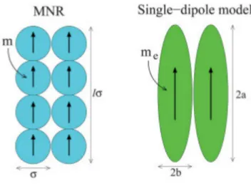
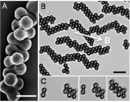
variety of structures and self-assembled patterns [35] (see Fig. 1.2.3). Compared with the individual magnetic particles, the collective behavior of rod-like particles is much less understood. Alvarez and Klapp [36], in a recent paper, analyzed the structure formation of a special class of rods by computer simulations using the Monte Carlo method. They quote the possibility of simulate such systems using a special class of magnetic nanorods (MNR) consisting of dipolar beads which are permanently linked to each other composing a stiff chain with internal head-to-tail alignment of the dipole moment (see Fig. 1.8). The first approach shown in Fig. 1.8(a) is based on recent experiments by Birringer et al. [37]. The authors performed a field assisted deposition technique to produce magnetic rods made of iron oxide beads aligned as illustrated in Fig. 1.9.
Figure 1.8: Two possible approaches to simulate nanorods: (a) MNR approach, where each particle has a diameter σ and dipole moment m, the lenght of each rod is lσ. (b) Spheroids with dipole moment me for minor radius b and the major radius a. Figure
extracted from Ref. [36].
Figure 1.9: Schematic representation of the experimental rods synthesis procedure. (a) The magnetic dipole moment (white arrows) are aligned to an external field H0 during
deposition. (b) Magnetic field assisted self-assembly of individual dipolar rods. The build-up of field gradients is symbolized by flux-lines. (c) Further growth of individual rods is accompanied by a change in growth mode resulting in the formation of bundles of rods. Figure extracted from Ref. [37].
1.3. LIQUID CRYSTALS-LIKE STATES 33
Figure 1.10: Peanut-shaped particles with a permanent transverse magnetic dipole. Figure extracted from Ref. [39].
Figure 1.11: Illustration of a formation of ribbon-like chains by magnetic rods with a non-axial dipole moment. Figure extracted from Ref. [40].
1.3
Liquid Crystals-Like States
positional order, but the molecules are oriented about a particular direction. Because of the anisotropy in the structure, these have interesting optical properties, i.e., they polarize light. This is why LC are useful for display technologies. Another type of LC is
Figure 1.12: Examples of Liquid crystals.
smetic. As the nematic phase, they have orientational order, however they also have some positional order, which is not necessarily in all directions as illustrated in Fig. 1.12(b). A smetic phase can be ordered in a particular direction but disordered in other. There is also an interesting variance of LC, which are the so-called cholesteric liquid crystals. In the cholesteric phase, the molecules are directionally oriented and stacked in a helical pattern, with each layer rotated at a slight angle with respect to the ones above and below it. The fundamental thing about LC is that they have orientational order but not always translational order. An important order parameter used to investigate the orientational order is the so-called nematic order parameter [41] related to the largest eigenvalue (G2)
of the following matrix:
Qkf =
1 2N
N
X
i
(3ˆsiksˆif −δkf), (1.9)
where i refers to particle i, the indexes k and f denote the cartesian components of the orientation vector s, N refers to the number of particles, and G2 is 0 for isotropic phase
2
Numerical Methods
The majority of the laws of nature is expressed by equations that one can hardly solve them exactly, but in very special conditions. However, it is possible to solve such equations with a good accuracy by using computers through numerical methods. For instance, much of the theoretical condensed matter physics, deals with systems consisting of many atoms and molecules. Such systems are not feasible to be studied analytically. Therefore, numerical methods applied in physical systems enables us to predict the be-havior of a system before it is studied experimentally. In this chapter we will discuss the computational methods that have enabled this work. A brief but not vague description of Molecular Dynamics Simulation will be presented.
2.1
Molecular Dynamics Simulation
Molecular dynamics (MD) is a computer simulation method, based on the physical equations of motion of the atoms and molecules in the context of N-body simulation. The atoms and/or molecules are allowed to interact to each other for a period of time reproducing the particle motion. The trajectories of atoms and molecules are determined by solving numerically the Newton’s equations for a system of interacting particles, where the forces between the particles and the potential energy are defined by the interatomic potentials or molecular mechanics force fields. Therefore, it is a deterministic method to simulate the physical system. The MD measurement approach is quite similar to the real experiment’s. We must first prepare the sample ofN particles, then we solve the Newton’s equations to know their time evolution, when the system reaches the equilibrium, all the averages of interest are performed. The motion equation can be written in several ways. Perhaps one of the most fundamental form is the Lagrangian equation of motion
d dt
∂L ∂q˙k
!
− ∂q∂L k
= 0, (2.1)
whereq and q˙ are the generalized coordinates and velocities of all particles, respectively,
2.1. MOLECULAR DYNAMICS SIMULATION 39
energies
L=K−V. (2.2)
By Legendre transformation, the Hamiltonian is obtained such as
H(p, q) = X
k
˙
qkpk−L(q,q˙), (2.3)
wherepk is the generalized momentum defined by
pk =
∂L ∂q˙k
. (2.4)
If the Hamiltonian is a purely quadratic function of the velocities and the potential energy does not depend on the velocities, the Hamiltonian will match the system total energy
H = 1 2 X i p2 i mi +X i<j
V(rij), (2.5)
whererij =|dxxˆ+dyyˆ|is the interparticle distance, andpiandmi are the momentum and
the mass of the i particle, respectively. In MD, we must take into account all the forces which all the particles are submitted. Once we know the interaction potential between the particles, we can obtain the interaction force by:
fij =−∇V. (2.6)
The net force in particle iis calculated in terms of their components
fxi =−
dx rij
∂V(rij)
∂r
!
, fyi =−
dy rij
∂V(rij)
∂r
!
, fzi =−
dz rij
∂V(rij)
∂r
!
. (2.7)
E.g., in the case that V(r) is equal to Eq. (1.8)
fx=
3µi·µj
r5
ij
−15(µi·rij)(µj ·rij)
r7
ij
+ 48ǫ
σ12 r14 ij dx+ 3 r5 ij
µjx(µi·rij) +µix(µj ·rij)
, (2.8)
fy =
3µi·µj
r5
ij −
15(µi·rij)(µi·rij)
r7
ij
+ 48ǫ
σ12 r14 ij dy+ 3 r5 ij
µij(µi·rij) +µiy(µj ·rij)
. (2.9)
Therefore, the equation of motion of each particle is given by
mi
d2r
i
dt2
!
=Fi =
N
X
j6=i
fij, (2.10)
For linear rigid bodies, e.g. rods, in addition to the forces, we must also take into account the torques. Considering that there are only two rotational degrees, the torque on a linear molecule can be written as a sum over a interaction sites
N=X
i
ri×fi =s×X
i
difi =s×G, (2.11)
where the orientation is defined bys, the unit vector along the molecular axis, and where di is the distance of each interaction site from the center of mass (CM), see Fig. 2.1. In
i
j
k
d
CM
is
Figure 2.1: Illustration of important parameters of a linear rigid body model.
the linear case, the angular momentum is simplyL=Iω, (I is the rod moment of inertia andω is the angular velocity), so that the equations of motion to the angular case, using
Eq. (2.11), are
Idω
dt =s×G, (2.12)
ds
dt =u =ω×s. (2.13) The quantity u is the tangential velocity, and it gives the information of how the orien-tation of the linear body, given by s, is changing over time. Thus, we can obtain the tangential acceleration(α) by doing the derivative of Eq. (2.13) with respect to the time
du
dt =α= dω
dt ×s+ω×u. (2.14) From Eq. (2.12) we have
α = 1
I(s×G×s) +ω×ω×s. (2.15) Using the identity of Eq. (A38), we have that
α = −I−1s(G·s) +I−1G(s·s)
| {z }
1
+ω(ω·s)
| {z }
0
−s(ω·ω)
| {z }
ω2
, (2.16)
2.1. MOLECULAR DYNAMICS SIMULATION 41
asω is perpendicular tos so,ω·s= 0. Doing the dot product of s and (−s(G·s) +G),
we can see that they are perpendicular to each other. So we can say that : G⊥ =
(−s(G·s) +G). For linear rods in a plane, ω =ωˆz and s=sxˆx+syˆy, then
u·u = (ω×s)·(ω×s),
= [ωzˆ×(sxxˆ+syyˆ)]·[ωzˆ×(sxxˆ+syyˆ)],
= ω2s2x+ω2sy2 =ω2(s2x+s2y
| {z }
1
) =ω2. (2.18)
Thus, using Eq. (2.17), the tangential acceleration for a linear rod in two-dimensions
α=I−1G⊥−s(u·u). (2.19)
2.1.1
Integration of The Equations of Motion
To integrate the equations of motion numerically, we will use the so-called Verlet-Scheme [8, 43], which we will focus on the Leapfrog method and the velocity Verlet method. Despite its low order, the Leapfrog method has excellent energy conservation properties and it is widely used. It is equivalent to Verlet Method [44]. The derivation of the Leapfrog method follows immediately from the Taylor expansion [45] of the coordinate variable -r(t)
r(t+δt) = r(t) +v(t)δt+ (δt2/2)f(t)
m +O(δt
3), (2.20)
wheref(t) is the force and m is the mass of the particle. We can rewrite Eq. (2.20) by
r(t+δt) = r(t) +δt
v(t) + (δt/2)f(t)
m
+O(δt3). (2.21)
The term multiplying δt is just the Taylor expansion of v(t+δt/2), and the truncation
error is on the order ofO(δt3). Similarly, if we subtract the Taylor expansion ofv(t−δt/2)
from the corresponding expression forv(t+δt/2)we have the complete integration leapfrog
scheme
v(t+δt/2) =v(t−δt/2) + f(t)
m δt, (2.22)
r(t+δt) = r(t) +v(t+δt/2)δt. (2.23)
The velocities and coordinates are evaluated at different times, but it does not denote a problem. In order to evaluate the instantaneous kinetic energy, we need the instantaneous velocityv(t), for this purpose we perform as the following equation
v(t) = 1
2(v(t+δt/2) +v(t−δt/2)). (2.24)
For the angular motion, we have similar equations from Eqs. (2.22) and (2.23), thus
From Eq. (2.25) we obtain
u(t−δt/2) =u(t)−δt
2α(t). (2.27)
We can obtain the relationu(t)·u(t)needed from Eq. (2.19) by doing the dot product of s(t)in both sides of Eq. (2.27) we have
s(t)·u(t−δt/2) = s(t)·u(t)−s(t)·I−1G⊥(t)−s(t) [u(t)·u(t)]
δt
2,
= −(u(t)·u(t))δt 2,
u(t)·u(t) = −2
δts(t)·u(t−δt/2), (2.28) where we useds(t)·s(t) = 1, s(t)·u(t) = 0 and s(t)·G⊥(t) = 0.
However, it is possible to cast an integration scheme which evaluates the positions and the velocities at the same instant of time. The so-called velocity Verlet algorithm also can be derived from a Taylor expansion
r(t+δt) =r(t) +v(t)δt+f(t) 2mδt
2, (2.29)
s(t+δt) =s(t) +u(t)δt+α(t)δt2. (2.30) The update of the velocities is given by
v(t+δt) =v(t) + f(t) +f(t+δt)
2m δt, (2.31)
u(t+δt) = u(t) + α(t+δt) +α(t)
2 δt. (2.32)
Eliminating the velocities in these equations will trace back to the original Verlet algorithm [43], so the original and the velocity version are completely equivalent. To calculate the trajectories and the orientations, the Eqs. (2.29) - (2.32) are processed gradually by the simulation program. Compared to other integrators with only one force evaluation like the Euler method with error on the orderδt2, the numerical stability of the Verlet algorithm
is much higher and the errors are of order δt2. From a physical point of view the time
reversibility is very important.
2.1.2
Periodic Boundary Conditions
2.1. MOLECULAR DYNAMICS SIMULATION 43
information in Refs. [46,47]. Because we are interested in bulk phases properties, it is not satisfactory to simulate the system as a closed box. In such a simulation box of a system of 1000 particles, arranged on a simple squared lattice, a not-neglected amount of particles are in contact with the surface of the box. These particles will experience quite different forces as particles inside the bulk. This problem can be overcome by implementing peri-odic boundary conditions (PBC). The small system of particles is expanded to infinity by surrounding the central simulation box with identical copies till an infinite space-filling array is obtained. It works as if the sample is simulated as a small piece within a larger portion of the same material. So if the particles leave the central simulation box, an image of their own will re-enter it directly through the opposite face. That is, if a particle in the integration step, leaves the simulation box through its right end by a distance δx, e.g., it will be replaced at a distance δx to the right from the left end of the box, while the positions of the other particles are held. The same goes for the interactions, as a direct consequence of periodic boundary conditions is theminimum image convention first used by Metropolis et al. in Monte Carlo (MC) simulations [48]. If all interactions between a central particle and the other particles in the box should be calculated in periodic systems, we have to take into account that some copies of particles are closer to the central one, than the particle itself. Once the particles are in the rightmost edge, e.g., they interact with the others as they are in the left extreme of the box as though they are in a box which is immediately to the left of the first one. This idea is extended to3D systems.
A two-dimensional system subjected to PBC is illustrated in Fig. 2.2. There are several boxes with length L, identical to the central one, periodically distributed around that. If a particle is located at ri relative to the center of the main box, then the system
will also recognize a set of ghost particles with locations given by ri+nL, where n ∈ Z,
so the potential energy is given by
U(ri, ..., rN) =
X
i<j
u(rij) +
X
n
X
i<j
u(|rij +nL|). (2.33)
The expression above presents a problem for systems with long-range interactions1, e.g., Coulomb interactions, because, in this case, Eq. (2.33) diverges. In terms of simulation for this type of system, we must use a technique to truncate the system energy. Among several methods, Ewald Sum [42] is the one of the most used. For systems with short-range interaction, we just need to worry about limiting the interactions of the particles that are within a region whose radius is called the cutoff radius. In general, the cutoff radius would be the distance which the interaction energy is very small, so that we can neglect the interactions of particles whose distance is greater than this cutoff range. In order the cutoff radius concept to work properly, one defines the size of the box as the double cutoff radius. Thus, the distance between a particle and its image will not be less than half of the size of the box. We are not going to go into the details of long-range
.
r
i
r
i+ L
L
Figure 2.2: Illustration of a 2D system subject to PBC. The yellow-shaded box represents the central (real) simulation box.
technique because in the 2D case, the dipolar pair interaction falls off fast ( r−3) and
therefore it is sufficient to take the simulation box sufficiently large such that no special long-range summation techniques is necessary.
2.1.3
Statistical Mechanics and Molecular Dynamics
MD simulations provide knowledge of the classical microscopic states of the system. Every microstate is represented by a particular point in phase space corresponding to a full set of generalized coordinates qj and conjugate momenta pj, Γ = (q1, ..., q6N, p1, ..., p6N)
composing a multidimensional space (see Fig. 2.3). A set of points Γ in the phase
2.1. MOLECULAR DYNAMICS SIMULATION 45
L
p
x
dp
(a)
p
x
E E+ Ed
(b)
Figure 2.3: Some examples of classic phase spaces - (a) Phase space of a free particle for
0< x < L and p, p+δp - (b) Phase space for harmonic oscillator with energy E, E+δE
is given by the ensemble average [49,50]
hAi=
R
A(Γ)ρ(Γ)dΓ
R
ρ(Γ)dΓ , (2.34)
where ρ(Γ) is the phase density. From a single system configuration/snapshot produced
by molecular dynamics simulation we can determine the instantaneous valueA(Γ). With
running simulation the system evolves in time, so that a trajectory in phase space Γ(t)is
produced and A(Γ(t))will change. To measure the observable macroscopic property Aobs
from simulation, we determine the time average over a definite time periodtobs
Aobs =< A(Γ(t))>= lim tobs→∞
1
tobs
Z tobs
0
A(Γ(t))dt. (2.35)
In general, time averaging should be done over infinite times to get macroscopic quantities, but in practice this might be satisfied with long enough finite times tobs. Since MD
simulation does not provide continuous time development of the system, we have to sum the instantaneous values ofAat integer multiples of the time stepδt. For instance, in the canonical ensemble (NVT), where the number of particles, volume and temperature are conserved, the ensemble average (in equilibrium) ofAcan be expressed in terms of phase space integrals taking into account the total potential energy of the system,U =U(rN),
as
hAi=
R
A(rN) exp−βU(rN)
drN
R
exp−βU(rN)
drN , (2.36)
where rN is the set of coordinates, Z =R exp−βU(rN)
points Γ), in the same instant of time, and make an average of all these states. So, it is
important to know the distribution of the pointsΓ in phase space. TheLiouville theorem [41] ensures that the distribution function of the phase space is constant over time. As a result, if there is a trajectory in the phase space that goes through all the points of it, so that ρens 6= 0, then, each system will eventually visit all states. Such a system is
called ergodic. This ensures the possibility of replacing the time average to an ensemble average. Therefore, the MD method is based on the assumption that the ergodic principle holds, and then the time that a particle spends in a given region of the phase space is proportional to the volume of this region. In other words, the ergodic principle states that all the accessible microstates are equally likely for the limit t → ∞. Consequently, the temporal average obtained in a MD run should be, in principle, the same as the ensemble average, i.e.
Aobs =
1
M
M
X
i=1
Ai(rN) =hAi, (2.37)
whereM is the total number of measurements for independent runs.
In general the ergodicity of a system has always to be proved for a definite set of parameters, but this is hard to do. In MD ergodicity is often destroyed by metastable states trapping the system for extended periods of time. This problem can be avoided by comparing averages of observables from different simulations with the same simulation parameters, but different initial configurations. Even in this case one cannot be sure, however, to reach every region in phase space.
2.1.4
Molecular Dynamics Scheme
A typical MD simulation run consists of the following basic steps:
1. Initialization of the system, i.e., assign initial coordinates and initial velocities for all the particles in the system;
2. Calculation of the interaction force between pairs of particles. This is the most time-consuming part of any MD simulation;
3. Numerical integration of the equation of motion by using a suitable scheme i.e., velocitity Verlet, leapfrog algorithm;
4. Apply the periodic boundary conditions, if necessary.
These are all done in one single time-step. If m is the total number of time-steps in the simulation, then ttot = mδt is the total time of the simulation run, and δt is the
2.1. MOLECULAR DYNAMICS SIMULATION 47
particle) over time and check if it has reached a stationary value, i.e., constant over time. The number of time-steps in order the system to reach this equilibrium situation depends on each problem specifically, therefore a careful analysis should be done for each particular case. The time interval between the beginning of the simulation and the equilibrium state is usually called the thermalization procedure. Only after the thermalization procedure one should calculate physical properties of interest, either structural properties (e.g., radial distribution function (RDF)) or dynamical properties (e.g., mean square displacement (MSD) and velocity autocorrelation function (VACF)).
2.1.5
Control of Temperature
One of the concerns when one performs MD simulation is to bring the system to the desired temperature as the system is in contact to a thermal reservoir. One of the most known controlling method is based on the rescaling of the velocities (v and u). The advantage of integration methods aforementioned is the possibility of adjusting the velocities of the particles straightforwardly according to the nominal temperature T0 of
the thermal reservoir
v(t+δt/2) =
s
T0
T(t)v(t−δt/2) + f(t)
m δt, (2.38)
where T(t) is the temperature at time (or step) t, this property is calculated based on the energy equipartition theorem, where each degree of freedom of the system contributes with kBT /2for the total energy. So, the instantaneous temperature is given by
T(t) =
N
X
i=1
mivα,i2 (t)
N kB
, (2.39)
wherevα,i is theα component of the velocity of i-th particle of a system withN particles.
In order to allow fluctuations of the kinetic energy, we can make the system to be weakly coupled to the heat bath. For this, a further refinement of the velocity rescaling approach has been proposed by Berendsen [51], at each time step, velocities are scaled by a factor
χ=
1 + δt
τ
T(t)
T0 −
1
−1/2
, (2.40)
2.1.6
Important Measured Quantities
Pair correlation function
A measurement for the structure of matter is the radial pair distribution functiong(r),
dependent only on the pair separation r for a translational invariant system of identical particles. It gives the probability of finding a pair of particles a distancer apart, relative to the probability expected for a completely random distribution for the same density. We get the radial pair distribution function by the definition [8]
g(r) = V
N2
* X
i
X
j6=i
δ(r−rij)
+
, (2.41)
where V is volume, N is the number of particles, rij is the i and j particles separation,
and h...i stands for an average over the realizations. From the point of view of statistical mechanics, where usually the number of degrees of freedom is large, the function represents an important physical measure to characterize structural properties of molecular systems, e.g., liquids, glasses and super-cooled liquids, etc. As rij = rji, which makes the Eq.
(2.41) to be reduced to
g(r) = 2V
N2
* X
i
X
j<i
δ(r−rij)
+
. (2.42)
2.1. MOLECULAR DYNAMICS SIMULATION 49
As ρ = N/V (N/A), for 3D (2D), and considering it constant, we get to, after a both sides integration
ρ
Z
g(r)dr= 2
N Z * X i X j<i
δ(r−rij)
+
=N −1, (2.43)
which is the result of counting the number of remaining particles around a chosen particle at the origin.
In terms of simulation, Eq. (2.42) is evaluated as a histogram in order to count the number of particles in a given shell of radius∆r, which is at a distancerfrom the reference (origin) particle (see Fig. 2.4). For a2Dsystem, considerhnthe number of pairs of atoms
(i, j) with the condition (n−1)∆r ≤ rij < n∆r. By counting the pair of atoms in the
shell ∆r, one would get [8]
g(rn) =
hn
πrnρ∆r
, (2.44)
wherern = (n−1/2)∆r and n is the index of the each bin of the histogram.
Clustering properties
Cluster formation is a very important subject of self-assembled systems, because is a real physical process and some models exhibit special properties to clusters. In MD simulations, it is important to be able to identify conditions which particles belong to a same cluster. Often it is used an energy criteria which considers two particles bonded when there is a attraction interaction between two particles. Another alternative method requires less computation effort based on the interparticle distance. The latter condition considers two particles bonded, let us say i and j, if their separation rij < δc, where δc
is the critical separation for two particles to be considered bonded. The value of δc is
typically based on energy conditions.
There are basically some quantities that help us to analyze the clustering properties. The so-called polymerization [58] evaluates the tendency of the system to form clusters and it is defined by
Φ = Nc N , (2.45)
whereNcis the number of clustered particles andN is the total number of particles. When
Φ = 1every particle belongs to a cluster, not necessarily the same. ForΦ = 0, in another
hand, it stands for a monomer phase. Another important quantity is the cluster size distribution n(s) (see Fig. 2.5). It is an important tool to identify percolated structures
since right at the percolation threshold, the cluster size distribution of an infinite system shows a power-law decayn(s)∼s−τ, whereτ is the so-called Fisher exponent that assumes
specific values for characteristic systems close to percolation transition, i.e, τ ∝ −187/91
(a)
(b)
Figure 2.5: (a) Cluster size distribution for packing fractionη= 0.01(ratio of the occupied
area over the available area) at several temperatures; (b) Cluster size distribution close to percolation (T = 0.078 and density ρ= 0.1). To minimize size effects, 40000particles
have been simulated. The different straight lines show the theoretical predictions for mean-field and 2d-percolation, as well as the best fitting slope of the numerical cluster distribution. The cluster size predicted by the Flory–Stockmayer (FS) theory [60] is also reported, but its range of validity is limited to only small clusters. ρ(s) stands for the
frequency of appearance ofs-sized cluster. Extracted from Ref. [61].
Percolation properties
2.1. MOLECULAR DYNAMICS SIMULATION 51
(b) (a)
Figure 2.6: (a) Percolation probability as a function of the volume fraction for different aspect ratio (l) and dipole moment (m). (b) Example of a 3D-percolated cluster system of nanorods. Extracted from Ref. [36].
Percolation on continuous systems was originally discussed as a phenomenon in the context of flow through a porous media, however the statistical theory of percolation has been used to understand the critical behavior of fluids. Percolation is defined according to the conventional method when at least50%of the sampled configurations in the simulation
trajectory contain a system-spanning cluster, i.e., the percolation probability is evaluated by counting the number of appearances of a cluster which spans over the system in a such way it is possible to make a continuum path through any sequence of bonds and any two opposite edges that limit the system. Under these circumstances, the cluster is effectively infinite when applying periodic boundary conditions. Typical percolating fluids exhibit a single peak in the cluster distribution comparable to the system size and these states are denoted as random percolated (see Fig. 2.7).


![Figure 2.3: Some examples of classic phase spaces - (a) Phase space of a free particle for 0 < x < L and p, p + δp - (b) Phase space for harmonic oscillator with energy E, E + δE is given by the ensemble average [49, 50]](https://thumb-eu.123doks.com/thumbv2/123dok_br/15639698.618652/45.892.211.730.133.437/figure-examples-classic-particle-harmonic-oscillator-ensemble-average.webp)