Evaluation of Constant Thickness Cartilage Models vs. Patient Specific Cartilage Models for an Optimized Computer-Assisted Planning of Periacetabular Osteotomy.

(1)

Evaluation of Constant Thickness Cartilage

Models vs. Patient Specific Cartilage Models

for an Optimized Computer-Assisted Planning

of Periacetabular Osteotomy

Li Liu1☯_{*, Timo Michael Ecker}2☯_{, Steffen Schumann}1_{, Klaus-Arno Siebenrock}2_,

Guoyan Zheng1

1Institute for Surgical Technology and Biomechanics, University of Bern, CH-3014, Bern, Switzerland, 2Department of Orthopaedic Surgery, Inselspital, Bern, Switzerland

☯These authors contributed equally to this work.

*li.liu@istb.unibe.ch

Abstract

Modern computerized planning tools for periacetabular osteotomy (PAO) use either mor-phology-based or biomechanics-based methods. The latter relies on estimation of peak contact pressures and contact areas using either patient specific or constant thickness carti-lage models. We performed a finite element analysis investigating the optimal reorientation of the acetabulum in PAO surgery based on simulated joint contact pressures and contact areas using patient specific cartilage model. Furthermore we investigated the influences of using patient specific cartilage model or constant thickness cartilage model on the bio-mechanical simulation results. Ten specimens with hip dysplasia were used in this study. Image data were available from CT arthrography studies. Bone models were reconstructed. Mesh models for the patient specific cartilage were defined and subsequently loaded under previously reported boundary and loading conditions. Peak contact pressures and contact areas were estimated in the original position. Afterwards we used a validated preoperative planning software to change the acetabular inclination by an increment of 5° and measured the lateral center edge angle (LCE) at each reorientation position. The position with the larg-est contact area and the lowlarg-est peak contact pressure was defined as the optimal position. In order to investigate the influence of using patient specific cartilage model or constant thickness cartilage model on the biomechanical simulation results, the same procedure was repeated with the same bone models but with a cartilage mesh of constant thickness. Com-parison of the peak contact pressures and the contact areas between these two different cartilage models showed that good correlation between these two cartilage models for peak contact pressures (r = 0.6342[0.6, 0.8], p<0.001) and contact areas (r = 0.872>0.8, p< 0.001). For both cartilage models, the largest contact areas and the lowest peak pressures were found at the same position. Our study is the first study comparing peak contact pres-sures and contact areas between patient specific and constant thickness cartilage models during PAO planning. Good correlation for these two models was detected. Computer

OPEN ACCESS

Citation:Liu L, Ecker TM, Schumann S, Siebenrock K-A, Zheng G (2016) Evaluation of Constant Thickness Cartilage Models vs. Patient Specific Cartilage Models for an Optimized Computer-Assisted Planning of Periacetabular Osteotomy. PLoS ONE 11(1): e0146452. doi:10.1371/journal. pone.0146452

Editor:Randy D Trumbower, Emory University School Of Medicine, UNITED STATES

Received:July 8, 2015

Accepted:December 17, 2015

Published:January 5, 2016

Copyright:© 2016 Liu et al. This is an open access article distributed under the terms of theCreative Commons Attribution License, which permits unrestricted use, distribution, and reproduction in any medium, provided the original author and source are credited.

Data Availability Statement:All relevant data are within the paper. All CT arthrography images used in our study are available from open source data provided by University of Utah (http://mrl.sci.utah.edu/ software/dysplastic-hips-image-data/).

(2)

assisted planning with FE modeling using constant thickness cartilage models might be a promising PAO planning tool when a conventional CT is available.

Introduction

Periacetabular osteotomy (PAO) is an established surgical intervention for treatment of hip

dysplasia and acetabular retroversion [1,2]. During the procedure, the acetabulum is

reori-ented in order to optimize the containment of the femoral head and the pressure distribution between acetabulum and femoral head for reduction of the peak contact pressures within the joint. The goal of acetabular reorientation is to restore or to approximate normal acetabular geometry. In order to achieve this, two types of planning strategies have been reported, which can be divided into morphology-based planning methods and biomechanics-based planning methods. Morphology-based planning uses standard geometric parameters, which have shown

their importance for quantification of acetabular under- or overcoverage [3]. Several authors

have described different morphology-based planning methods which range from simplified

two-dimensional planning [4–6] to complex three-dimensional planning applications [7–11].

Other authors presented biomechanics-based planning methods. Different approaches have

been presented using for example Discrete Element Analysis (DEA) [12], or the more

sophisti-cated Finite Element Analysis (FEA) [13,14]. In literature, both constant thickness cartilage

models [14] and patient specific cartilage models [15] have been suggested. In the clinical

rou-tine, knowledge of patient specific cartilage is rarely available, since special imaging protocol (e.g. CT arthrography or MRI with dGEMRIC, T1rho or T2 mapping) is necessary to retrieve this information. One alternative could be constant thickness cartilage model that is virtually generated from bony surface models derived from conventional CT scans. However differences between these two different cartilage models in planning of PAO using FE simulation have never been investigated. Previously, we have developed a morphology-based 3D planning

sys-tem for PAO [16]. This system allows for quantification of the hip joint morphology in three

dimensions, using geometric parameters such as inclination and anteversion angle, the lateral center edge (LCE) angle and femoral head coverage. It also allows for virtual reorientation of the acetabulum according to these parameters. In the current study, we enhanced this applica-tion with an addiapplica-tional biomechanics-based method for estimaapplica-tion of joint contact pressures employing FEA. In this study, we investigated the following research questions:

1. What is the optimal position of the acetabulum based on simulated joint contact pressures using patient specific cartilage models in a FE analysis?

2. Are there significant differences in joint contact pressures between patient specific cartilage model and constant thickness cartilage model in the same hip model?

Materials and Methods

System Overview

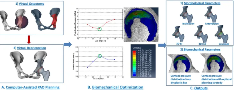
The computer-assisted planning system for PAO uses 3D surface models of the pelvis and the femur, generated out of DICOM (digital imaging and communication in medicine) data, using a commercially available segmentation program (AMIRA, Visualization Sciences Group, Bur-lington, MA). The system starts with a morphology based method. Employing fully automated detection of the acetabular rim, parameters such as acetabular version, inclination, LCE angle,

data collection and analysis, decision to publish, or preparation of the manuscript.

(3)

femoral head extrusion index (EI), femoral head coverage can be calculated for a

computer-assisted diagnosis [16]. Afterwards, the system offers the possibility to perform a virtual

osteot-omy (Fig 1.A(1)) and reorientation of the acetabular fragment in a stepwise pattern. During

the fragment reorientation, acetabular morphological parameters are re-computed in real-time

(Fig 1.A(2)) until the desired position is achieved.

Our system is further equipped with a biomechanics-based FE prediction of changes of car-tilage contact stresses, which occurs during acetabular reorientation. An optimal position of the acetabulum can be defined, once contact areas in the articulation are maximized, while at

the same time peak contact pressures are minimized (Fig 1.(B)).

The respective cartilage model for the biomechanics-based FE prediction is generated from either CT arthrography data (patient specific) or using a virtually generated cartilage with pre-defined thickness (constant thickness).

Biomechanical Model of Hip Joint

Cartilage models. In literature, both constant thickness cartilage models and patient

spe-cific cartilage models have been employed. Zou et al. [14] used a constant thickness model and

thus created a cartilage with a predefined thickness of 1.8mm, a value derived from cartilage

thickness data from the literature. In contrast Harris et al. [15] introduced a CT arthrography

protocol allowing for excellent visualization of patient specific cartilage. DICOM data of dys-plastic hip joints, which have been CT scanned using this arthrography protocol were provided by the open source dysplastic hips image data from the Musculoskeletal Research Laboratories,

University of Utah [17]. The data provider has obtained IRB approval (University of Utah IRB

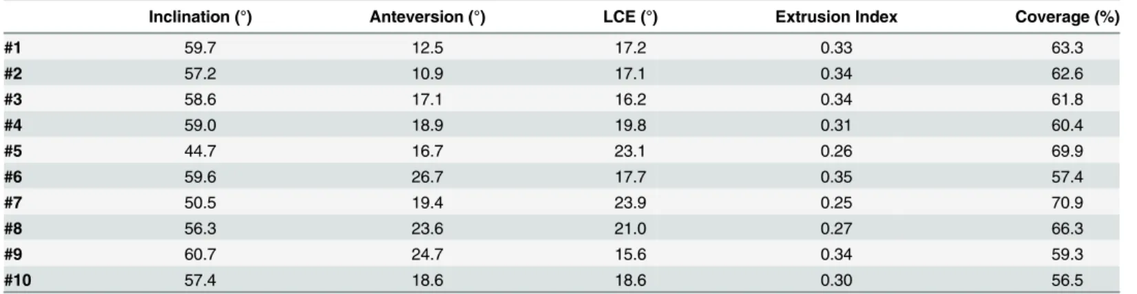
#10983). We used our morphology-based planning system for calculation of the acetabular

morphological parameters [18], verifying true dysplasia (Table 1). We used these datasets in

order to retrieve the patient specific cartilage models. The bony anatomy of the same ten speci-men was then used to create the constant thickness cartilage models by expanding a constant 1.8mm thickness using 3D dilation operation on the articular surface.

Fig 1. The schematic workflow of computer assisted planning of PAO with biomechanical optimization.(A) Computer assisted morphology based PAO planning. Virtual osteotomy operation is done with a sphere, whose radius and position can be interactively adjusted, and virtual reorientation operation is done by interactively adjusting anteversion and inclination angle of the acetabulum fragment. (B) Biomechanical optimization. (C) the pre-operative planning output.

(4)

Mesh Generation. Bone and cartilage surface models of the reoriented hip joints were

imported into ScanIP software (Simpleware Ltd, Exeter, UK) as shown inFig 2(A) and 2(C).

Surfaces were discretized using tetrahedral elements (Fig 2(B) and 2(D)). Since the primary

focus were the joint contact stresses, a finer mesh was employed for the cartilage than for the

bone. Refined tetrahedral meshes were constructed for the cartilage models (*135369

ele-ments for the femoral cartilage model, and*92791 elements for the acetabular cartilage

model, using the ScanFE module (Simpleware Ltd, Exeter, UK). Cortical bone surfaces were

discretized using coarse tetrahedral elements (*149120 elements for the femoral model, and

*188526 elements for the pelvic model). Trabecular bone was not included in the models, as it

only has a minor effect on the predictions of contact pressure as reported in another study [19].

Table 1. Acetabular morphological parameters of ten specimen with hip dysplasia.

Inclination (°) Anteversion (°) LCE (°) Extrusion Index Coverage (%)

#1 59.7 12.5 17.2 0.33 63.3

#2 57.2 10.9 17.1 0.34 62.6

#3 58.6 17.1 16.2 0.34 61.8

#4 59.0 18.9 19.8 0.31 60.4

#5 44.7 16.7 23.1 0.26 69.9

#6 59.6 26.7 17.7 0.35 57.4

#7 50.5 19.4 23.9 0.25 70.9

#8 56.3 23.6 21.0 0.27 66.3

#9 60.7 24.7 15.6 0.34 59.3

#10 57.4 18.6 18.6 0.30 56.5

doi:10.1371/journal.pone.0146452.t001

Fig 2. Biomechanical simulation of contact pressure on acetabular cartilage.(A) Surface models of a dysplastic hip; (B) Volume meshes of a dysplastic hip. (C) Surface models for a planned situation after acetabulum fragment reorientation. (D) Volume meshes for the planned situation. (E) Boundary conditions and loading for biomechanical simulation. (F) Coarse meshes for bone models, and refined meshes for cartilages.

(5)

Material property. Acetabular and femoral cartilage were modeled as homogeneous,

iso-tropic, and linearly elastic material with Young’s Modulus E = 15 MPa and Poisson’s ratioν=

0.45 [14]. Cortical bone of pelvis and femur were modeled as homogeneous, isotropic material

with elastic modulus E = 17 GPa and Poisson’s ratioν= 0.3 [14].

Boundary Conditions and Loading. Tied and sliding contact constraints were used in Abaqus/CAE 6.10 (Dassault Systèmes Simulia Corp, Providence, RI, USA) to define the carti-lage-to-bone and cartilage-to-cartilage interfaces, respectively. It has been reported that the

friction coefficient between articular cartilage surfaces was very low (0.01–0.02) in the presence

of synovial fluid, making it reasonable to neglect eventual frictional shear stresses [15,20]. The

top surface of pelvis and pubic areas were fixed, and the distal end of the femur was constrained to prevent displacement in the body x and y directions while being free in vertical z direction

(Fig 2(E)). The center of the femoral head was derived from a least-squares sphere fitting and

was selected to be the reference node. The nodes of femoral head surface were constrained by the reference node via kinematic coupling. The fixed boundary condition model was then

sub-jected to a loading condition as published before [21], representing a single leg stance situation

with the resultant hip joint contact force acting at the reference node. Following the loading

specifications suggested in another previous study [22](Fig 2(E)), the components of joint

con-tact force along 3 axes were given as 195N, 92N, and 1490N, respectively. In order to remove any scaling effect of body weight on the absolute value of the contact pressure, we defined a constant body weight of 650N for all subjects. The resultant force was applied, based on

ana-tomical coordinate system described by Bergmann et al [21], whose local coordinate system

was defined with the x axis running between the centers of the femoral heads (positive running from the left femoral head to the right femoral head), the y axis pointing directly anteriorly, and the z axis pointing directly superiorly.

Study 1: FE Simulation for biomechanics-based planning of PAO using patient specific cartilage model. In order to find the optimal aceatbular position, the acetabular fragment was

now virtually rotated around the y axis (Fig 2(E)) in 5° increments in relation to the anterior

pel-vic plane (APP). This deemed to imitate a decrease in actabular inclination, as performed during

actual PAO surgery (Fig 2(C)). For each increment, the predicted peak contact pressure and

total contact area were directly extracted from the output of Abaqus/CAE 6.10. The resulting peak contact pressures and contact areas in the different acetabular positions were then com-pared and the corresponding LCE angle were measured. Optimal orientation was determined by the position yielding the maximum contact area and the minimum peak contact pressure.

Study 2: Evaluation the influences of using different cartilage models on the simulation results. After the peak pressures and contact areas had been simulated using the patient spe-cific cartilage models, the same procedure was performed using the constant thickness cartilage models. Finally, comparison between peak pressures and contact areas between patient specific and constant thickness cartilage models was performed. Linear regression analysis was used to determine associations between the results for peak pressures and contact areas for both carti-lage types. Thus, the values for the constant thickness models were the independent variables, whereas the values obtained by the patient specific models represented the dependent variables.

Pearson’s correlation coefficient r was interpreted as“poor”below 0.3,“fair”from 0.3 to 0.5,

“moderate”from 0.5 to 0.6,“moderately strong”from 0.6 to 0.8, and“very strong”from 0.8 to

1.0. Significance level was defined as p<_0.05.

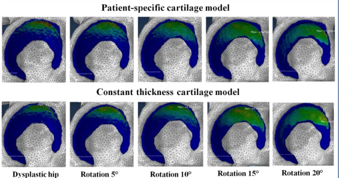
Results

(6)

homogeneously distributed contact area (Fig 3). At the same time, an increase in LCE angle resulted in decreased peak contact pressures. For each specimen, the optimal acetabular frag-ment reposition was defined as the position with minimum peak contact pressure and

maxi-mum contact area (Table 2).

Comparison of the peak contact pressures and the contact areas between the two different

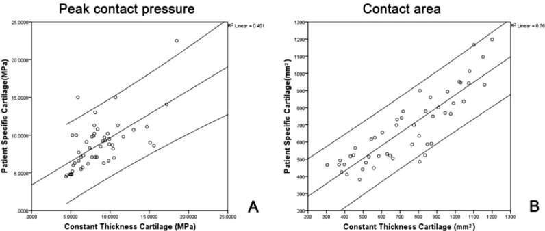
cartilage models showed similar results (Table 3). Regression analysis quantitatively showed

that the results obtained by the constant thickness cartilage models had good correlation with those obtained by using the patient specific cartilage models. Specifically, a moderately strong correlation was found between both cartilage models when analyzing peak contact pressures

(r = 0.6342_{[0.6, 0.8], p}<_{0.001) (}_{Fig 4}_{) while a very strong correlation was also found when}

analyzing the contact areas between the two different cartilage models (r = 0.872>0.8,

p<_{0.001) (}_{Fig 4(B)}_{). For both cartilage models, the largest contact areas and the lowest peak}

pressures were found at the same position (Table 3)

Discussion

We used a previously validated morphology-based PAO planning system [16] to perform

vir-tual acetabular reorientation. An additional biomechanics-based module then estimated con-tact areas and peak concon-tact pressures within the joint. First we used hip joint models with patient specific cartilage models and changed the LCE angle in order to increase femoral head containment and to find the optimal position with the largest contact area and lowest peak contact pressure. The same operation was then conducted with the bone models of the same hip joints by replacing the patient specific cartilage models with virtually generated constant thickness cartilage models. In the patient specific cartilage models an increase in LCE angle led to an enlarged and more homogeneously distributed contact areas and decreased peak contact pressures. Comparison of the peak contact pressures and the contact areas between the two dif-ferent cartilage models showed similar results. Regression analysis quantitatively showed

Fig 3. Contact pressure distribution obtained by using two different cartilage models at different acetabular reorientation position.

(7)

moderately strong correlation between both models for peak contact pressures while very strong correlation for contact areas.

In the light of our findings, several aspects need to be discussed. We did not include the ace-tabular labrum in our FE analysis, however the role of the labrum during load distribution is

debatable in literature. While some authors promoted inclusion of the labrum [23], other

authors denied the importance of its inclusion [24]. More interestingly, Henak et al. [17] showed

that the labrum has a far more significant role in dysplastic hip joints biomechanics than it does in normal hips, since it supports a large percentage of the load transferred across the joint due to

the eccentric loading in dysplastic hips. The same study group in a previous study [25], however,

found that the labrum only supported less than 3% of the total load across the joint in normal hips. The final goal of our study was not to measure peak contact pressures and contact areas in

the originally dysplastic state of our specimen, but to find an optimal position resembling a“

nor-mal”hip joint during PAO. Hence, for this purpose disregarding the labrum was acceptable.

Table 2. Acetabular fragment reposition position with peak contact pressures and contact area.

R-0° R-5° R-10° R-15° R-20°

#1 LCE (°) 17.2 23.0 27.9 32.9* 37.9

Peak contact pressure (MPa) 14.1 9.5 7.1 4.8* 7.3

Contact area (mm2) 523 616 778 899* 860

#2 LCE (°) 17.1 21.7 26.8_* 31.8_* 36.8

Peak contact pressure (MPa) 8.7 6.6 6.3* 7.0 9.8

Contact area (mm2) 625 655 698 741* 731

#3 LCE (°) 16.2 19.9 24.4* 29.4 34.5

Contact area (mm2₎ ₇₇₉ ₈₉₄ ₁₀₁₃_* ₉₄₇ ₉₄₃

#4 LCE (°) 19.8 23.5* 28.0 33.0 38.0

Peak contact pressure (MPa) 7.1 6.2* 8.3 10.2 13.0

Contact area (mm2₎ ₁₁₆₆ ₁₁₉₈

* 1096 933 836

#5 LCE (°) 23.1 27.9 32.9* 37.9 43.0

Contact area (mm2) 636 769 764* 587 523

#6 LCE (°) 17.7 21.5 26.5_* 31.6_* 36.6

Contact area (mm2) 466 493 517 565* 468

#7 LCE (°) 23.9 28.9 33.9* 38.9* 43.9

Peak contact pressure (MPa) 11.3 9.8 10.0* 10.0* 15.0

Contact area (mm2₎ ₄₄₁ ₅₂₁ ₅₈₆ ₅₉₀_* ₄₈₅

#8 LCE (°) 21.0 26.0 31.0 36.0* 41.0

Contact area (mm2₎ ₄₆₉ ₅₁₄ ₅₁₈ ₅₃₀

* 505

#9 LCE (°) 15.6 19.6 24.6 29.7* 34.7

Contact area (mm2) 425 381 411 480* 448

#10 LCE (°) 18.6 23.0 28.0_* 32.8 37.8

Contact area (mm2) 802 826 951* 750 699

*represents the position with minimum peak contact pressure and maximum contact area.

(8)

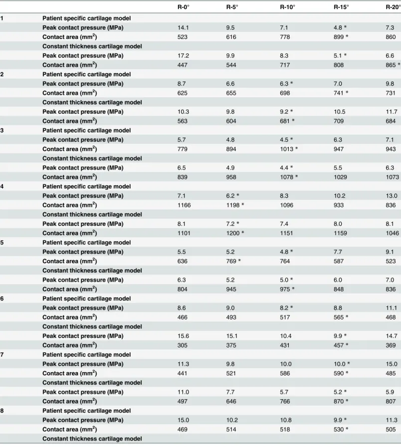
Table 3. Acetabular fragment reposition position with peak contact pressures and contact area (Patient specific cartilage model vs. Constant thick-ness cartilage model).

R-0° R-5° R-10° R-15° R-20°

#1 Patient speciﬁc cartilage model

Contact area (mm2) 523 616 778 899* 860

Constant thickness cartilage model

Contact area (mm2₎ ₄₄₇ ₅₄₄ ₇₁₇ ₈₀₈ ₈₆₅_*

Contact area (mm2₎ ₆₂₅ ₆₅₅ ₆₉₈ ₇₄₁

* 731

Contact area (mm2) 563 604 681* 709 684

Contact area (mm2) 779 894 1013* 947 943

Contact area (mm2₎ ₈₃₉ ₉₅₈ ₁₀₇₈_* ₁₀₂₉ ₁₀₇₃

Contact area (mm2₎ ₁₁₆₆ ₁₁₉₈

* 1096 933 836

Contact area (mm2) 1101 1200* 1151 1159 1046

Contact area (mm2) 636 769* 764 587 523

Contact area (mm2₎ ₈₀₄ ₉₄₅ ₉₇₅_* ₈₄₈ ₈₃₆

Contact area (mm2₎ ₄₆₆ ₄₉₃ ₅₁₇ ₅₆₅

* 468

Contact area (mm2) 305 375 431 457* 369

Contact area (mm2) 441 521 586 590* 485

Contact area (mm2₎ ₄₉₇ ₆₄₆ ₇₆₆ ₈₇₀_* ₈₀₇

Contact area (mm2₎ ₄₆₉ ₅₁₄ ₅₁₈ ₅₃₀

* 505

(9)

Regarding loading conditions, a fixed body weight of 650N [21] was used, which is not

patient specific. However, Zou et al. [14] justified the use of constant loading, since the relative

change of contact pressure before and after PAO reorientation planning is assessed, regardless the true patient weight. Also, the applied loading conditions were derived from in vivo data

from patients who underwent total hip arthroplasty (THA) [21] and thus might be just an

approximation to the true loading conditions in the native joint. For simplification reasons we also did not simulate typical motion patterns such as sitting-to-standing or gait cycle. Since we Table 3. (Continued₎

R-0° R-5° R-10° R-15° R-20°

Contact area (mm2₎ ₃₉₈ ₅₃₁ ₅₈₄ ₆₃₀ ₆₆₁_*

Contact area (mm2₎ ₄₂₅ ₃₈₁ ₄₁₁ ₄₈₀

* 448

Contact area (mm2) 383 481 412 515 558*

Contact area (mm2₎ ₈₀₂ ₈₂₆ ₉₅₁_* ₇₅₀ ₆₉₉

Contact area (mm2₎ ₉₀₉ ₉₉₀ ₁₀₂₁_* ₈₇₉ ₇₇₅

*represents the position with minimum peak contact pressure and maximum contact area.

doi:10.1371/journal.pone.0146452.t003

Fig 4. (A) Scatter plot of peak contact pressure obtained by constant thickness cartilage models against those obtained by patient specific cartilage models. (B) Scatter plot of contact area obtained by constant thickness cartilage models against those obtained by patient specific cartilage models.

(10)

only performed static loading, the conchoid shape of the hip joint, which is important, when performing dynamic loading, was also disregarded. This might be a limitation, when interpret-ing our results. Finally, although the CT scans were performed in the supine position and the

loading condition is based on one-leg stance situation, this is not an infrequent practice [26]

and previous work [27] has shown that there was no significant difference between the contact

pressure in the one-leg stance reference frame and those in the supine reference frame.

Our results are reflected conclusively in the current literature. Zhao et al. [13] conducted a

3D FE analysis investigating the changes of Von Mises stress distribution in the cortical bone before and after PAO surgery. They showed the favorable stress distribution in the normal hips compared to dysplastic hips. One limitation of this study might be, that the specimens were not truly dysplastic hips. The authors created dysplasia by deforming the acetabular rim of nor-mal hip joints. Hence, their depiction of the stress distribution in the dysplastic joint is rather an approximation. Furthermore, they used a constant thickness cartilage model. They did not estimate pressure distribution in the cartilage model but in the underlying subchondral cortical

bone. Another group developed a biomechanical guiding system (BGS) [12,26,28]. In 2009

they presented a manuscript reporting on three-dimensional mechanical evaluation of joint contact pressure in 12 PAO patients with a 10 year follow-up. They measured radiologic angles and joint contact pressures in these patients pre- and postoperatively. The authors were able to show that after 10 year follow-up, peak contact pressures were reduced 1.7-fold and that lateral coverage increased in all patients. One limitation of their study is the use of discrete element analysis (DEA). Since the system was not only used for preoperative planning, but also as an intraoperative guidance system, the DEA represents a computationally-efficient method for modeling of cartilage stress by neglecting underlying bone stress. The cartilage models however remain largely approximated, since neither patient specific nor constant cartilage models are used, but a simplified distribution of spring elements is employed for cartilage simulation.

Recently, Zou et al. [14] also developed a 3D FE simulation of the effects of PAO on contact

stresses. They validated their method on 5 models generated from CT scans of dysplastic hips and used constant thickness cartilage models. The acetabulum of each model was rotated in 5° increments in the coronal plane from the original position and the relationship between con-tact area and pressure, as well as Von Mises stress in the cartilage were investigated, looking for the optimal position for the acetabulum. One limitation of this study is, that acetabular

reorien-tation was roughly performed with a commercial FE analysis software (Abaqus1, Dassault

Sys-tèmes Simulia Corp, USA). Unlike our morphological-based planning application, their method is thus unvalidated and does not have a precise planning tool for an accurate quantifi-cation of patient specific 3D hip joint morphology.

In conclusion, our investigation contributes well to the current state of the art. First, to the best knowledge of the authors, this is the first study to use a patient specific cartilage model for biomechanics-based planning of PAO allowing for estimation of changes of contact areas and peak pressures in truly dysplastic hips. Previous studies had either investigated normal or dys-plastic hips, but never the true change during virtual reorientation of the latter. Furthermore, our results seems conclusive, since the optimal position with the largest contact areas and

low-est peak pressures were found within the predefined normal values [3,29] for the investigated

LCE angle. This range for safe positioning is especially important, since in real-time surgery

reorientation towards the one“perfect”position might not be feasible. Finally, the comparison

(11)

investigation is needed, computer assisted planning with FE modeling using constant thickness cartilage might be a promising PAO planning tool providing conclusive and plausible results.

Acknowledgments

First and second author contributed equally during conduction of this study, analysis of the data and assembly of the manuscript. This work was supported the open source dysplastic hips

image data from the University of Utah [17] and partially supported by the Japanese-Swiss

Sci-ence and Technology Cooperation Program.

Author Contributions

Conceived and designed the experiments: GZ LL TME KAS. Performed the experiments: LL. Analyzed the data: LL TME. Contributed reagents/materials/analysis tools: LL SS. Wrote the paper: LL TME GZ. Designed the software used in analysis: LL SS.

References

1. Ganz R, Klaue K, Vinh TS, Mast JW. A New Periacetabular Osteotomy for the Treatment of Hip Dyspla-sias Technique and Preliminary Results. Clinical orthopaedics and related research. 1988; 232:26–36.

PMID:3383491

2. Steppacher SD, Tannast M, Ganz R, Siebenrock KA. Mean 20-year followup of Bernese periacetabular osteotomy. Clinical orthopaedics and related research. 2008; 466(7):1633–1644. doi: 10.1007/s11999-008-0242-3PMID:18449617

3. Tannast M, Hanke MS, Zheng G, Steppacher SD, Siebenrock KA. What are the radiographic reference values for acetabular under-and overcoverage? Clinical Orthopaedics and Related Research1

. 2015; 473(4):1234–1246. doi:10.1007/s11999-014-4038-3

4. Tannast M, Siebenrock KA, Anderson SE. Femoroacetabular impingement: radiographic diagnosis—

what the radiologist should know. American Journal of Roentgenology. 2007; 188(6):1540–1552. doi: 10.2214/AJR.06.0921PMID:17515374

5. Tannast M, Mistry S, Steppacher SD, Reichenbach S, Langlotz F, Siebenrock KA, et al. Radiographic analysis of femoroacetabular impingement with Hip2Norm-reliable and validated. Journal of Orthopae-dic Research. 2008; 26(9):1199–1205. doi:10.1002/jor.20653PMID:18404737

6. Clohisy JC, Carlisle JC, Trousdale R, Kim YJ, Beaule PE, Morgan P, et al. Radiographic evaluation of the hip has limited reliability. Clinical orthopaedics and related research. 2009; 467(3):666–675. doi: 10.1007/s11999-008-0626-4PMID:19048356

7. Klaue K, Wallin A, Ganz R. CT evaluation of coverage and congruency of the hip prior to osteotomy. Clinical orthopaedics and related research. 1988; 232:15–25. PMID:3383480

8. Millis MB, Murphy SB. Use of computed tomographic reconstruction in planning osteotomies of the hip. Clinical orthopaedics and related research. 1992; 274:154–159. PMID:1729000

9. Dutoit M, Zambelli P. Simplified 3D-evaluation of periacetabular osteotomy. Acta Orthop Belg. 1999; 65 (3):288–294. PMID:10546351

10. Janzen D, Aippersbach S, Munk P, Sallomi D, Garbuz D, Werier J, et al. Three-dimensional CT mea-surement of adult acetabular dysplasia: technique, preliminary results in normal subjects, and potential applications. Skeletal radiology. 1998; 27(7):352–358. doi:10.1007/s002560050397PMID:9730324

11. Dandachli W, Kannan V, Richards R, Shah Z, Hall-Craggs M, Witt J. Analysis of cover of the femoral head in normal and dysplastic hips NEW CT-BASED TECHNIQUE. Journal of Bone & Joint Surgery, British Volume. 2008; 90(11):1428–1434. doi:10.1302/0301-620X.90B11.20073

12. Armand M, Lepistö J, Tallroth K, Elias J, Chao E. Outcome of periacetabular osteotomy: joint contact pressure calculation using standing AP radiographs, 12 patients followed for average 2 years. Acta orthopaedica. 2005; 76(3):303–313. PMID:16156455

13. Zhao X, Chosa E, Totoribe K, Deng G. Effect of periacetabular osteotomy for acetabular dysplasia clari-fied by three-dimensional finite element analysis. Journal of orthopaedic science. 2010; 15(5):632–640.

doi:10.1007/s00776-010-1511-zPMID:20953924

(12)

15. Harris MD, Anderson AE, Henak CR, Ellis BJ, Peters CL, Weiss JA. Finite element prediction of carti-lage contact stresses in normal human hips. Journal of Orthopaedic Research. 2012; 30(7):1133–

1139. doi:10.1002/jor.22040PMID:22213112

16. Liu L, Ecker T, Schumann S, Siebenrock K, Nolte L, Zheng G. In: Computer assisted planning and navi-gation of periacetabular osteotomy with range of motion optimization. Springer; 2014. p. 643–650.

17. Henak CR, Abraham CL, Anderson AE, Maas SA, Ellis BJ, Peters CL, et al. Patient-specific analysis of cartilage and labrum mechanics in human hips with acetabular dysplasia. Osteoarthritis and Cartilage. 2014; 22(2):210–217. doi:10.1016/j.joca.2013.11.003PMID:24269633

18. Liu L, Ecker T, Xie L, Schumann S, Siebenrock K, Zheng G. Biomechanical validation of computer assisted planning of periacetabular osteotomy: A preliminary study based on finite element analysis. Medical Engineering & Physics. 2015;. doi:10.1016/j.medengphy.2015.09.002

19. Anderson AE, Ellis BJ, Maas SA, Peters CL, Weiss JA. Validation of finite element predictions of carti-lage contact pressure in the human hip joint. Journal of biomechanical engineering. 2008; 130 (5):051008. doi:10.1115/1.2953472PMID:19045515

20. Caligaris M, Ateshian GA. Effects of sustained interstitial fluid pressurization under migrating contact area, and boundary lubrication by synovial fluid, on cartilage friction. Osteoarthritis and Cartilage. 2008; 16(10):1220–1227. doi:10.1016/j.joca.2008.02.020PMID:18395475

21. Bergmann G, Deuretzbacher G, Heller M, Graichen F, Rohlmann A, Strauss J, et al. Hip contact forces and gait patterns from routine activities. Journal of biomechanics. 2001; 34(7):859–871. doi:10.1016/ S0021-9290(01)00040-9PMID:11410170

22. Phillips A, Pankaj P, Howie C, Usmani A, Simpson A. Finite element modelling of the pelvis: inclusion of muscular and ligamentous boundary conditions. Medical engineering & physics. 2007; 29(7):739–

748. doi:10.1016/j.medengphy.2006.08.010

23. Ferguson S, Bryant J, Ganz R, Ito K. An in vitro investigation of the acetabular labral seal in hip joint mechanics. Journal of biomechanics. 2003; 36(2):171–178. doi:10.1016/S0021-9290(02)00365-2

PMID:12547354

24. Konrath GA, Hamel AJ, Olson SA, Bay B, Sharkey NA. The Role of the Acetabular Labrum and the Transverse Acetabular Ligament in Load Transmission in the Hip*. The Journal of Bone & Joint Sur-gery. 1998; 80(12):1781–8.

25. Henak CR, Ellis BJ, Harris MD, Anderson AE, Peters CL, Weiss JA. Role of the acetabular labrum in load support across the hip joint. Journal of biomechanics. 2011; 44(12):2201–2206. doi:10.1016/j. jbiomech.2011.06.011PMID:21757198

26. Armiger RS, Armand M, Tallroth K, Lepistö J, Mears SC. Three-dimensional mechanical evaluation of joint contact pressure in 12 periacetabular osteotomy patients with 10-year follow-up. Acta orthopae-dica. 2009; 80(2):155–161. doi:10.3109/17453670902947390PMID:19404795

27. Niknafs N, Murphy RJ, Armiger RS, Lepistö J, Armand M. Biomechanical factors in planning of periace-tabular osteotomy. Frontiers in bioengineering and biotechnology. 2013; 1. doi:10.3389/fbioe.2013. 00020PMID:25152876

28. Lepistö J, Armand M, Armiger RS. Periacetabular osteotomy in adult hip dysplasia–developing a

com-puter aided real-time biomechanical guiding system (BGS). Suomen ortopedia ja traumatologia = Orto-pedi och traumatologi i Finland = Finnish journal of orthopaedics and traumatology. 2008; 31(2):186. PMID:20490364

29. Haefeli P, Steppacher S, Babst D, Siebenrock K, Tannast M. An Increased Iliocapsularis-to-rectus-femoris Ratio Is Suggestive for Instability in Borderline Hips. Clinical Orthopaedics and Related Research1_{. 2015; 473(12):3725}