THE ROLE OF ARTIST AND GENRE ON MUSIC EMOTION RECOGNITION

i

THE ROLE OF ARTIST AND GENRE ON

MUSIC EMOTION RECOGNITION

Pedro Miguel Fernandes Vale

ii

NOVA Information Management School

Instituto Superior de Estatística e Gestão de Informação

Universidade Nova de Lisboa

THE ROLE OF ARTIST AND GENRE ON

MUSIC EMOTION RECOGNITION

by

Pedro Miguel Fernandes Vale

Dissertation presented as partial requirement for obtaining the Master’s degree in Information Management, Specialization in Knowledge Management and Business Intelligence.

Supervisor: Prof. Dr.Rui Pedro Paiva

iii

ABSTRACT

The goal of this study is to classify a dataset of songs according to their emotion and to understand the impact that the artist and genre have on the accuracy of the classification model. This will help market players such as Spotify and Apple Music to retrieve useful songs in the right context.

This analysis was performed by extracting audio and non-audio features from the DEAM dataset and classifying them. The correlation between artist, song genre and other audio features was also analyzed. Furthermore, the classification performance of different machine learning algorithms was evaluated and compared, e.g., Support Vector Machines (SVM), Decision Trees, Naive Bayes and K-Nearest Neighbors.

We found that Support Vector Machines attained the highest performance when using either only Audio features or a combination of Audio Features and Genre. Namely, an F-measure of 0.46 and 0.45 was achieved, respectively. We concluded that the Artist variable was not impactful to the emotion of the songs.

Therefore, by using Support Vector Machines with the combination of Audio and Genre variables, we analyzed the results and created a dashboard to visualize the incorrectly classified songs. This information helped to understand if these variables are useful to improve the emotion classification model developed and what were the relationships between them and other audio and non-audio features.

KEYWORDS

iv

Table of Contents

1. INTRODUCTION 1

1.1.BACKGROUND AND PROBLEM IDENTIFICATION 1

1.2.OBJECTIVES AND APPROACHES 2

2. LITERATURE REVIEW 3

2.1.MUSIC AND EMOTION 3

2.2. EMOTION PARADIGMS 5

2.2.1.CATEGORICAL PARADIGM 5

2.2.2.DIMENSIONAL PARADIGM 8

2.3. GENERAL MER REVIEW 10

2.3.1.RESEARCH REVIEW 10

2.3.2.ARTIST AND GENRE REVIEW 14

2.3.3.MERDATASETS REVIEW 16

2.3.4.MERAUDIO FRAMEWORKS REVIEW 24

2.3.5.AUDIO FEATURES REVIEW 27

3. IMPLEMENTATION 37

3.1. PRE-PROCESSING THE DATASET 37

3.2. CLASSIFICATION 48

3.3. VISUALIZATION 52

4. RESULTS AND DISCUSSION 54

4.1. FEATURE SELECTION 54

4.2. CLASSIFICATION RESULTS 55

4.3. GRID SEARCH IMPROVEMENTS 57

4.4. ARTIST VARIABLE WITH THE 2ND _{APPROACH 59}

4.5. CLASSIFICATION USING SVM 61

4.6. ANALYSIS OF INCORRECTLY CLASSIFIED SONGS 63

4.6. DASHBOARD 64

5. CONCLUSIONS AND FUTURE WORK 66

5.1.FUTURE WORK 66

6. BIBLIOGRAPHY 67

v

LIST OF FIGURES

FIGURE 1-HEVNER’S MODEL (HEVNER,1935) ... 6

FIGURE 2-RUSSELL’S MODEL OF EMOTION (CALDER,LAWRENCE,&YOUNG,2001) ... 9

FIGURE 3-TELLEGEN-WATSON-CLARK MODEL OF EMOTION (TROHIDIS,TSOUMAKAS,KALLIRIS,&VLAHAVAS,2011) 9 FIGURE 4-QUADRANT DISTRIBUTION OF SONGS WITH LESS THAN 51%AGREEMENT RATE ... 19

FIGURE 5-GENRE DISTRIBUTION OF SONGS WITH LESS THAN 51%AGREEMENT RATE... 20

FIGURE 6-LOWER-THAN-AVERAGE ENERGY FRAMES HIGHLIGHTED ON ENERGY CURVE (LARTILLOT,2013) ... 27

FIGURE 7-ATTACK TIME DETECTION (LARTILLOT,2013) ... 29

FIGURE 8-ATTACK SLOPE EXAMPLE (LARTILLOT,2013) ... 29

FIGURE 9-ZERO CROSSING RATE WAVEFORM (LARTILLOT,2013) ... 29

FIGURE 10-SPECTRAL ROLL OFF WITH FREQUENCY (LARTILLOT,2013) ... 30

FIGURE 11-SPECTRAL ROLL OFF USING PERCENTAGE (LARTILLOT,2013) ... 31

FIGURE 12-SENSORY DISSONANCE DEPENDING ON FREQUENCY RATIO (LARTILLOT,2013) ... 32

FIGURE 13-FUNDAMENTAL FREQUENCY (F0) AND RESPECTIVE MULTIPLES (LARTILLOT,2013) ... 34

FIGURE 14-TONAL CENTROID FOR A MAJOR TRIAD IS SHOWN AT POINT A(LEE,2008) ... 35

FIGURE 15-RUSSEL’S CIRCUMPLEX MODEL (Y.-H.YANG ET AL.,2008)... 38

FIGURE 16- QUADRANT DISTRIBUTION OF SONGS ... 39

FIGURE 17-GENRE DISTRIBUTION OF SONGS ... 42

FIGURE 19-QUADRANT DISTRIBUTION OF SONGS ... 48

FIGURE 20–BACKWARDS FEATURE SELECTION FOR AUDIO,GENRE AND ARTIST MODEL ... 54

FIGURE 21-NUMBER OF SONGS PER ARTIST USING 2ND APPROACH... 60

FIGURE 22–MODEL’S CONFUSION MATRIX ... 62

vi

LIST OF TABLES

TABLE 1-THE FIVE MIREX CLUSTERS AND RESPECTIVE SUBCATEGORIES (MALHEIRO,2016)... 6

TABLE 2-COMPARISON OF EMOTION MODELS ... 10

TABLE 3-ORIGINAL VERSUS REPLICATED MODEL RESULTS COMPARISON ... 21

TABLE 4 –VARIABLES FOR THE FINAL MODEL ... 47

TABLE 5-F-MEASURE RESULTS COMPARISON BEFORE GRID-SEARCH ... 56

TABLE 6-F-MEASURE RESULTS COMPARISON AFTER GRID-SEARCH IMPROVEMENTS ... 57

TABLE 7-F-MEASURE RESULTS COMPARISON BETWEEN ARTIST VARIABLE APPROACHES ... 61

vii

LIST OF EQUATIONS

EQUATION 1–ANNOTATIONS AGREEMENT RATE (%) ... 18

EQUATION 2–ROOT-MEAN-SQUARE ENERGY ... 27

EQUATION 3–ZERO CROSSING RATE ... 30

EQUATION 4–SPECTRAL ROLL OFF ... 30

EQUATION 5–SPECTRAL FLUX ... 31

EQUATION 6–SPECTRAL PEAKS VARIABLITY ... 32

EQUATION 7–SPECTRAL CENTROID ... 32

EQUATION 8–SPECTRAL CREST FACTOR ... 33

EQUATION 9–SPECTRAL FLATNESS MEASURE ... 33

EQUATION 10–PEARSON’S CORRELATION COEFFICIENT ... 40

EQUATION 11–MIN-MAX NORMALIZATION ... 41

EQUATION 12-F-MEASURE METRIC ... 51

EQUATION 13–PRECISION METRIC ... 51

EQUATION 14–RECALL METRIC ... 51

viii

ACRONYMS

Term Definition

BPM Beats per minute

DEAM Database for Emotional Analysis in Music

GEMS Geneva Emotional Music Scale

KNN K-Nearest Neighbours

MER Music Emotion Recognition

MFCC Mel-Frequency Cepstral Coefficient

MIR Music Information Retrieval

MIREX Music Informational Retrieval Evaluation eXchange

NA Negative Affect

NB Naive Bayes

PA Positive Affect

RBF Radial Basis Function

RMS Root-Mean-Square Energy

SFM Spectral Flatness Measure

1

1.

INTRODUCTION

Music is an important part of one’s individual and collective culture. It is used to carry emotions from the composer to the listener (Hevner, 1935).

Nowadays, music is a colossal industry with global revenues of 28.7 billions of dollars in 2015, a growth of 11.6% compared with the former fiscal year (Ellis-Petersen, 2016). Spotify and Apple offer consumers a new way to listen to music: music streaming. In 2015, these streamers observed a 66% growth in subscriptions and helped the digital sales outperform the physical sales for the first time (Ellis-Petersen, 2016). These companies created enormous databases of songs, listeners and their preferences, and now have the need to retrieve the right song at the right time to the right listener.

1.1. Background and Problem Identification

The digital era brought numerous opportunities to the music business, expanding exponentially the number of data stored on the listener’s behaviors and tastes. Music streamers can now collect data while we listen to music in our car, while working, exercising, and during other activities by using their services.

The growth led to every person having a considerable collection of albums and songs. With the opportunities arrived the limitations of music cataloging and retrieval, which is still a relatively new area of research. The problem is retrieving relevant songs in a given context from gigantic databases (Panda, 2010).

This is the problem that the Music Information Retrieval (MIR) field of research tries to solve. There is a great effort in analyzing similar listeners to suggest new songs (Hu & Liu, 2010) but MIR researchers go a step further and analyze audio, melodic features and lyrics (Panda, Rocha, & Paiva, 2015).

Music Emotion Recognition (MER) is a relatively new field which investigates what emotions each song carries on to the listener. One of the problems is the non-existence of a universal definition of Emotion. Psychologists have made efforts to create frameworks in which we could classify emotions, but there is not a consensus yet (Kleinginna & Kleinginna, 1981).

2 Spotify, Pandora and other major players on the music industry are now sponsoring MIR and MER events held by the International Society of Music Information Retrieval. Spotify’s Weekly Discover Playlists, which suggest to listeners songs related to the ones they listened in the pasted by using emotion classification models and user-related metrics, had 1.7 billion streams in the first six months since it was created (Pasick, 2015).

One feature that have not been studied extensively was the Artist that created the song. Some artists have the habit of creating uplifting songs, while others prefer sad songs. The relationship between Artist, Genre and other audio and melodic features are an important step towards understanding which Emotion is expressed in the song.

1.2. Objectives and Approaches

The main objective is to analyze what is the impact that Artist and Genre have on the Music Emotion Recognition model when combined with other audio features. By creating multiple classification models with audio features and non-audio features, we aim to offer a contribution to understanding what is the role of the Artist and Genre variables on the overall classification model.

Secondly, we will analyze the correlation between Audio variables, Genre and Artist to observe which are the relationships between these song features.

Thirdly, even though there have been researches pointing that Support Vector Machines (SVM) outperform other Machine Learning algorithms, we will compare SVM with Decision Trees, Naive Bayes and K-Nearest Neighbors (Laurier & Herrera, 2007).

3

2.

LITERATURE REVIEW

2.1.

Music and Emotion

Since the main goal of this research is to study the role of emotions in music, it is important to have a clear definition of emotions and which are the main differences between the former and moods.

Kleinginna andKleinginna (1981) studied the definitions of emotion in order to find a universal terminology. They came up with the following definition: “Emotion is a complex set of interactions among subjective and objective factors, mediated by neural/hormonal systems, which can (a) give rise to affective experiences such as feelings of arousal, pleasure/displeasure; (b) generate cognitive pro-cesses such as perceptually relevant effects, appraisals, labelling propro-cesses; (c) activate widespread physiological adjustments to the arousing conditions; and (d) lead to behaviour that is often, but not always, expressive, goal-oriented, and adaptive.” (Kleinginna & Kleinginna, 1981).

The American Oxford Dictionary1 defines emotions as “A strong feeling deriving from one's circumstances, mood, or relationships with others.”. This means that one of the factors that influences emotions are moods. The definition of mood from the American Oxford Dictionary is “a temporary state of mind and feeling”.

One person can be sad for days, having this mood without any apparent reason. This mood will influence the appearance of emotions like angriness and sadness. “The concept of mood is com-plex and difficult to establish. It reflects a moving notion that cannot be easily grasped. (...) The con-ception of mood in cognitive psychology is derived from the analysis of emotion. While emotion is an instantaneous perception of a feeling, mood is considered as a group of persisting feelings associated with evaluative and cognitive states which influence all the future evaluations, feelings and actions” (Amado-Boccara, Donnet, & Olié, 1993). As stated, moods are difficult to define just like emotions.

It is important to differentiate these two concepts since both have a similar meaning. This differ-ence can help explain their own definition:

• Duration: Emotions have a shorter duration when compared to moods; • Intensity: Emotions are more intense than moods;

• Cause: Emotions can be aroused from moods while mood causes are usually unknown; • Strength: Emotions are stronger than moods.

1

4 When one watches his favorite movie or listens to his favorite song, an emotion will arise from the joy (mood). In this example, the cause was joy and the emotion happiness arouse from it. Emotions are stronger than moods because, when we are in a bad mood, we can still have moments of happi-ness. Emotions and moods are usually used interchangeably on the MIR research but we will opt to use the term Emotions, as we consider that it is the most accurate in the context of MER, where short music clips are considered.

Furthermore, in MER, emotions are commonly divided into three categories: expressed emotions, perceived emotions and induced emotions (Gabrielsson, 2001):

• Expressed emotion indicates the emotion that the performer wants to share with the listeners(Gabrielsson & Juslin, 1996);

• Perceived emotion refers to the emotions the listeners apprehend as being present in the song, which is not always equal to the expressed emotion or the emotion felt by the listener (Gabrielsson & Juslin, 1996);

• Induced emotion regards the emotion the listener feels in response to a song (Scherer & Zentner, 2001), i.e., the emotion felt while listening to the song.

Wager et al. determined that perception and induction of emotions are associated with ´peak activations’ in different areas of the brain, demonstrating that these are two distinct processes (Wager et al., 2008). These two categories of emotions do not have always a positive relation. There can also be negative, no systematic relation or no relation at all (Gabrielsson, 2001). MIR researches tend to focus on the perceived emotion, mainly because it is less dependable to situational factors (Y.-H. Yang & Chen, 2012). One performer might attempt to create a music that will transmit sadness, but the listener might perceive calmness, despite actually making him feel happier. We will focus on perceived emotions in this research.

5

2.2. Emotion Paradigms

In the literature, emotion models fall into two main paradigms: the dimensional and the cate-gorical paradigms. The main difference between them is the usage of discrete categories to represent emotions in the categorical models, while dimensional models represent emotions along 2 or 3 axes as discrete adjectives or as continuous values (Kim et al., 2010; Russell, 1980).

2.2.1. Categorical Paradigm

In this paradigm, two of the first and most well-known models are Hevner’s and Ekman’s. Ekman defended the existence of six categories, named ‘basicemotions’, which are the basis for the non-basic emotions (Ekman, 1992). The basic emotions, anger, disgust, fear, happiness, sadness and surprise, were developed according to facial expressions, which means that some of them (e.g., disgust) do not suit music well. There is also the issue of not having moods associated to music (e.g., calm) (Hu & Downie, 2010).

This representation is questioned by Ortony et al. (1990), who compare the notion of ‘basic emotions’ to ‘basic natural languages’. According to them, there are not basic natural languages, what exists is a great diversity of natural languages depending of the culture and other factors (Ortony & Turner, 1990).

Kate Hevner is one of the first researchers of music psychology. She concluded that music al-ways carries emotional meaning and that this meaning is not entirely subjective, so it can have some reason to it. Hevner’s model consists of eight clusters using a total of 67 adjectives (emotions) orga-nized in a circular way (Figure 1). Inside each cluster, adjectives have a close meaning (intra-cluster similarity). Distant clusters are less similar than adjacent clusters (e.g., the adjectives joyous (cluster 6) and humorous (cluster 5) have more similarities than the adjective joyous (cluster 6) and dreamy (clus-ter 3)) (Hevner, 1935).

6

Figure 1 - Hevner’s Model (Hevner, 1935)

MIREX (Music Information Retrieval Evaluation eXchange) is a framework used by the Music Information Retrieval (MIR) scientific community for the evaluation of systems and algorithms (Downie, 2008). This framework classifies songs into one of five clusters shown in Table 1.

Table 1 - The five MIREX clusters and respective subcategories (Malheiro, 2016)

7 To address the specific needs of induced emotions, which none of the mentioned above mod-els did, Zentner et al. (2008) developed a domain-specific scale named Geneva Emotional Music Scale (GEMS). Zentner et al. conducted four studies: the objective of the first and second studies was to create a list of terms for both perceived and felt emotions in which the conclusion was that the five groups of listeners evaluated showed a considerable variability across musical genre and perceived vs induced emotions. The difference was higher on the positive emotions in induced emotions. “As peo-ple move into a mental state in which self-interest and threats from the real world are no longer rele-vant, negative emotions lose their scope.” This remark by Zentner et al. is the justification on why induced emotions tend to be more positive. On the third and fourth studies, the researchers used factory analysis of questionnaire data of music-induced emotions to create the GEMS scale. Further factor-analysis added shorter versions of the 45 terms of the GEMS scale. The 9-term scale, which is one of the shorter versions, include the following terms: Wonder, Tenderness, Transcendence, Nos-talgia, Power, Peacefulness, Joyful, Tension, Activation and Sadness (Zentner, Grandjean, & Scherer, 2008).

Coutinho & Scherer (2012), confirmed the structure of GEMS with an experiment in which the problem of overrepresentation of classical music on the original research was addressed. New terms were suggested related to feelings of harmony, interest and boredom (Coutinho & Scherer, 2012).

Aljanaki (2016) points out that the conclusion in the original work, in which it is showed that the GEMS scale is a more precise instrument to measure musical emotion than Valence-Arousal or basic emotions, can be questioned. The main reasons are the small size of the experiment, the overrepresentation of one genre and the unconventionality of the questions regarding the Valence-Arousal model (Aljanaki, 2016).

8

2.2.2. Dimensional Paradigm

In this paradigm, the authors propose the use of a multi-dimensional space in order to plot the locations of the emotions. Commonly, a two-dimension approach is adopted, comprising two axes: arousal against valence. The Y-axis represents arousal (also known as energy, activation and stimula-tion level), and the X-axis represents valence (polarity of the emostimula-tion, also known as pleasantness, either positive or negative). This creates a four-quadrant interpretation corresponding to different emotions (Russell, 1980), as illustrated in Figure 2.

There is also a variation which includes a third dimension: dominance or potency, in order to differentiate between close emotions (e.g., fear (negative dominance) and anger (positive dominance) have similar arousal and valence values and, hence, might be distinguished by dominance) (Tellegen & Clark, 1999). For the sake of simplicity and visualization, MER works usually do not apply this dimen-sion.

Dimensional models can be further divided into discrete and continuous models. Discrete models address the representation of the emotion on one of the four quadrants, each having more than just one emotion (e.g., happiness and surprise are both high arousal and valence, belonging in the first quadrant). Continuous models approach each point on the continuous space as one emotion, reducing the ambiguity present on the discrete models. The two most well-known models are Russel’s Model and Tellegen-Watson-Clark’s Model.

9

Figure 2 - Russell’s Model of Emotion (Calder, Lawrence, & Young, 2001)

Tellegen-Watson-Clark’s Model is composed of a third dimension, and follows an innovative hierarchical perspective. A three-level hierarchy composed on the highest level by pleasantness vs un-pleasantness, an independent positive affect (PA) versus negative affect (NA) dimension at the second level, and discrete expressivity factors of joy, sadness, hostility, guilt/shame, fear emotions at the base level (Figure 3) (Tellegen & Clark, 1999).

Despite the lack of differentiation of close points (emotions) on the valence-arousal plan, it compensates in simplicity when compared with the third-dimensional models.

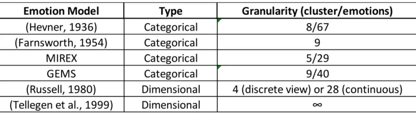
10 A brief summary of the models discussed above is presented in Table 2:

Table 2 - Comparison of emotion models

2.3. General MER Review

2.3.1. Research Review

Whilst being a relatively new research field, Music Emotion Recognition (MER) gained interest from researchers of diverse backgrounds.

The first paper on emotion detection in audio, to the best of our knowledge, was published by Feng et.al (2003). A system for emotion detection in music using only features of tempo and articula-tion was proposed to identify emoarticula-tions in a music piece. The categorical classificaarticula-tion model included only four emotions: happiness, anger, sadness and fear and it was performed using a neural network with three layers. The accuracy of the model of the happiness, sadness and anger categories was con-siderable, between 75% and 86%. On the other hand, the observed accuracy of the fear category was only of 25% (Feng, Zhuang, & Pan, 2003). The main issue with this research is that the sample is too small, with a collection of 330 songs for training and only 23 for testing, which is less than 7% of the total. Another problem can arise from the lack of representation of the fear category on the test data, with only 3 songs. There is also an absence of relevant information regarding the annotation process details and about the musical genres.

Li et al. (2003) were one of the first researchers to address MER as a multi-label classification problem by analyzing music signals. Multi-label classification regards songs as having the possibility to being associated with more than one emotion. As stated in the paper “In emotion detection in music, however, the disjointness of the labels is no longer valid, in the sense that a single music sound may be classified into multiple emotional categories.” The process was divided into feature extraction and multi-label classification. The authors used the Farnsworth adjective groups, which is a categorical

Emotion Model

Type

Granularity (cluster/emotions)

(Hevner, 1936)

Categorical

8/67

(Farnsworth, 1954)

Categorical

9

MIREX

Categorical

5/29

GEMS

Categorical

9/40

11 model, and added three additional groups: mysterious/spooky, passionate and bluesy. This adjective groups were grouped into six supergroups. The dataset consisted of 499 sound files extracted from 128 albums. Thirty audio features were extracted using the Marsyas software framework, belonging to three different categories: timbral texture features, rhythmic content features, and pitch content features. In order to build the classifiers, the authors used SVM. The dataset was divided into 50% training data and 50% test data, resulting in an F-measure micro average of 44.9% and a 40.6% macro average. The main problems with the article are within the dataset: the songs dataset was labeled by a single subject. In addition, only some genres were represented on the dataset: Ambient (120 files), Classical (164 files), Fusion (135 files), and Jazz (100 files) (Li & Ogihara, 2003).

Later that year, Liu et al. (2003) used a hierarchical framework against a non-hierarchical framework to classify acoustic music data using audio features: intensity, timbre and rhythm. The au-thors decided to use Thayer’s model of mood as the emotion framework and the 800 twenty seconds long music clips were labeled by three music experts. The results ranged from 76.6% to 94.5% for the hierarchical framework and from 64.7% to 94.2% for the non-hierarchical framework (D. Liu, Lu, & Zhang, 2003). The main limitation of this study is the fact that the scope of the classifier is restricted to classical acoustic music.

Aiming to increase efficiency in the annotation process, Yang et al. (2004), used a dataset of 152 Alternative Rock music samples of 30 seconds each, of which 145 had lyrics, to extract emotion intensity information. The focus of the research were the negative emotions, since the authors con-sidered them to be more ambiguous. The Tellegen-Watson-Clark’s mood model was used. The corre-lation between emotion intensity and rhythm and timbre features was 0.9. In order to separate like-valenced emotions, lyrics were used and observed an accuracy of 82.8% (D. Yang & Lee, 2004).

Yang et al. (2008) tried to predict arousal and valence values, using Russel’s model of mood. The dataset consisted of 195 songs from Western, Japanese and Chinese albums, which were distrib-uted uniformly in each quadrant of the emotion plane. The authors used Support Vector Regressions to estimate valence and arousal values, employing features such as pitch, timbral texture and pitch content. The R2 statistic observed was 58.3% for arousal and 28.1% for valence. Even though the au-thors demonstrated with Principal Component Analysis that valence and arousal were not truly de-pendent, the residual dependence can be deteriorating the accuracy of the model (Y.-H. Yang et al., 2008).

12 the emotion from 100 songs belonging to 7 different genres: Classical, Reggae, Rock, Pop, Hip-Hop, Techno and Jazz (Trohidis et al., 2011).

Bischoff et al. (2009), incorporated audio features with social annotations from Last.fm2 and compared the accuracy of the model against labels from AllMusic3, which are annotated by music ex-perts. The 4737 song’ dataset was evaluated using 3 different models: audio-based using SVM, tag-based using Naive Bayes and a linear combination of the former. The emotions were predicted accord-ing to MIREX, Thayer’s mood models and theme’s manual clusters from AllMusic. Audio features in-cluded BPM, MFCCs and spectral centroid. The highest accuracy was found in the theme’s clusters under the linear combination of social tags and audio features with an average accuracy of 62.5%. The labels used from Last.fm can have accuracy issues since any user can create these tags and associate them with a song. Likewise, as stated by the authors, the mood-related labels are less frequent on the platform, where users usually give more attention to the creation of genre-related labels (Bischoff et al., 2009). Also, the annotation process in AllMusic is unclear, namely, it is unclear if the annotators are focused on the audio part, lyrics part or both.

Recently, Song et al. (2012), studied which musical features are more relevant for emotion classification. The analysis of 2904 pop songs was conducted using SVM classifiers associated with two kernels: polynomial and radial basis functions. The results were trained and evaluated against Last.fm tags and audio data from 7digital4. The authors used a recent categorical emotional model named Geneva Emotion Musical Scale (GEMS). This study found that, by combining spectral, rhythmic and harmonic features, the model presented the best accuracy of 54% (Song, Dixon, & Pearce, 2012). One limitation of this work, in the context of our research, is that the GEMS model aims at induced emo-tions rather than perceived emoemo-tions.

Other features besides audio started being used in MIR and MER. Laurier et al. (2008) com-bined Natural Language Processing techniques on lyrics and MIR techniques on audio features. The assumption of this study was that part of the semantic information were present solely on the lyrics, hence it will be beneficial to add lyrics to the classification model. The research was divided into 3 models: audio-only, text-only and a bi-modal classification system integration of the two former mod-els. The authors used a categorical emotion model with the following categories: happy, sad, angry and relaxed, corresponding to each of the four Russell’s quadrants. Each category is binary, so one

13 song can be either ‘sad’ or ‘notsad’. The dataset is a collection of mainstream popular music and the selection was made using Last.fm tags and lyrics from LyricWiki5. Lastly, the listeners were asked for validation of the song’s emotion, and only songs that were validated by at least one listener were kept on the dataset. The final dataset was composed of 1000 songs. In order to classify the songs, three algorithms were compared: SVM, Logistic Regression and Random Forest. SVM performed better than the rest. The audio features used for the classification model were: timbral (e.g., spectral centroid), rhythmic (e.g., tempo), tonal (Harmonic Pitch Class Profiles) and temporal descriptors. The classifica-tion model with the best accuracy was the combinaclassifica-tion of audio and lyrics, showing considerably higher accuracy, reaching the peak difference around 5 percentage points in the categories ‘sad’ and ‘happy’, when compared with the audio-only and lyrics-only model. The authors mitigated the risk of error on the Last.fm tags by using the listener’s manual validation. Most studies referred above which used Last.fm as a source for social tags, did not use this methodology. Despite this, the annotations were only made by listening to 30 seconds of each song, creating the possibility of a biased analysis (Laurier et al., 2008).

In another study using lyrics as a feature of the emotion classification model, Hu et al. (2010) used a dataset of 5,296 songs to study lyrics versus audio-based models. Russel’s emotion model was selected and the songs were divided into 18 mood categories according to the tags generated by Last.fm users. Each mood categories were treated with a binary approach. From the 18 mood catego-ries, 7 divergent categories have shown lyrics outperforming audio features and only 1 category where audio features had a better performance. It was also demonstrated that the lyrics have a strong se-mantic connection with the mood categories (Hu & Downie, 2010). The main problem with this study is that the ‘groundtruth’ used was solely Lasfm.com tags and reviewed by two experts, which could be biased.

MIDI has been shown to be a good choice in order to have impact on the accuracy of emotion classification models, in particular on the valence dimension (Yi Lin, Chen, & Yang, 2013). Lu et al. (2010), extracted features from MIDI files such as Duration, Voice Separation, Acoustic Guitar Friction and Average Melodic Interval, to compare with audio feature and lyrics-based models. The authors used Thayer’s mood model and Adaboost to train a classifier that combined audio, lyrics and MIDI features. The dataset consisted of 500 Chinese pop songs labeled by 8 participants. The observation of the accuracy comparison between MIDI-only, lyrics-only, audio-only and the combined model shows that the combination of features is the most accurate model (72.4%). In the comparison results, it is

5

14 shown that the combination between audio and lyrics has an accuracy of 72%, which is only 0.4 per-centage points lower than the best model, which is the combination of lyrics, audio and MIDI. This can hint that there is redundancy in the information between audio and MIDI features. Secondly, the da-taset was comprised solely of Chinese pop songs, which makes it difficult to compare this paper’s model with other models developed mainly for Western songs (Lu, Chen, Yang, & Wang, 2010).

Besides standard audio features, lyrics and MIDI features, recently Panda et al. (2015) devel-oped a classification model with Standard and melodic audio features. The authors built the dataset extracted from AllMusic API to be close to MIREX Mood Classification Task, a categorical model which has five clusters. The dataset consisted of 903 audio-clips of 30 seconds each. Melodic features ex-tracted included pitch and duration features, vibrato features and contour typology. The best score resulted from using only 11 features with a F-measure of 64%. The conclusion was that the best results appear to be when there was a combination of melodic and standard audio features (Panda et al., 2015).

The best score obtained in the MIREX Audio Music Mood Classification Task, which is a com-petition held every year where researchers classify a dataset unknown to contestants, was observed in 2011 with a classification accuracy of 69.5%. We can compare different years because the dataset remained the same since the inception of the contest6.

2.3.2. Artist and Genre Review

In the artist and genre field, there is not a considerable amount of research. We will dive deeper into the three most well-known studies in this specific part of MER.

Exploiting Genre for Music Emotion Classification (Yu-ching Lin, Yang, Chen, Liao, & Ho, 2009)

This research uses a two-layer emotion classification scheme: in the first-layer the genre sification model takes place and in the second-layer the authors apply the genre-specific emotion clas-sification model.

The dataset is composed of 1535 songs collected from 300 albums and enriched with infor-mation from the review website AllMusic: 12 emotions and 6 genres. Each of the albums can have more than one emotion but can only have a single associated genre. Songs are converted to 22050Hz,

6

15 mono channel PCM WAV and feature extraction was done using Marsyas. The software extracted 436 audio features.

The authors prove through the Chi-Squared test of association that genre and emotion are not independent.

Firstly, a model of genre classification was created. Afterwards, on the second layer, one emo-tion classifier was used for each genre. Each classifier was used to classify songs inside each genre. For example, if a song is classified as Jazz on the first layer, the emotion will be classified in the second layer using the emotion classifier trained with Jazz songs.

On the first layer, for genre classification, LIBSVM was used. To evaluate the multi-label classi-fier, macro average F-measure and micro average F-measure were used. Macro average treats each label equally and Micro average regards the overall prediction result across all labels.

The authors demonstrated that, even with the first layer genre classifier errors (58.98% accu-racy), the accuracy on the second layer was higher than if the genres were known prior to the classifi-cation. The two-layer model had a macro average F-measure of 43% against 31% of the traditional model; and micro average F-measure of 56% against 52% of the traditional model.

Automatic Classification of Musical Mood by Content-Based Analysis (Laurier, 2011)

This thesis aimed to show the relationship between genre and emotion in the songs to improve emotion classification models.

The dataset consisted in 81749 tracks enriched with emotion labels from Last.fm database. By running dissimilarity tests in the emotion clusters, the authors decided to use a model of 4 emotion clusters: happy, sad, angry and calm/relaxed. The genre of these tracks was added through information sourced from the iTunes Music Store. Most of these tracks, 34.49% to be precise, belonged to the ‘Rock’ genre. Other genres included Reggae, Jazz, Electronic and Classical.

The machine learning algorithm chosen was SVM and the first conclusion reached was the observation of a high association between emotion and genre. Both positive and negative emotion categories are positively correlated with genres.

16 As it happens with other papers in MER, the use of Last.fm database can be problematic in terms of bias of the emotions used as ‘groundtruth’, because anyone can add labels to the songs on the online platform.

Exploring Mood Metadata: Relationships with Genre, Artist and Usage Metadata (Hu & Downie, 2007)

The main objective of this work is to demonstrate the relationships between emotion and art-ist, genre, and usage metadata. Usage metadata refers to the situations where the songs are adequate (e.g., Go to sleep, Driving).

The primary dataset for this study was AllMusic, composed of 179 emotion labels across 7134 albums and 8288 song, and the secondary datasets were extracted from epinions.com (for usage metadata) and Last.fm (for external corroboration).

A categorical model was used to classify the emotions in which there were 5 clusters each with 5 emotions.

In order to test the significance of the relationship between emotion and artist, genre and usage, the authors decided to use Fisher’s Exact Test (FET).

After testing the AllMusic dataset, the same study was conducted using the Last.fm dataset, to see if the results corroborated. The authors discovered that the genre-emotion and artist-emotion relationship can be generalizable to other datasets while the usage-emotion is more dependable and vulnerable to the vocabulary present in the datasets.

The authors concluded that the genre-emotion and artist-emotion relationships were robust and show promise on its use on the MIREX task. On the other hand, the usage-emotion relationship is not robust enough to be used.

As reported on the paper, the AllMusic has a data sparseness problem since some emotions are represented on more than 100 albums while others are associated with only 3 albums or songs.

2.3.3. MER Datasets Review

17 difficult to compare different MER studies, since researchers do not use the same dataset. The most used dataset for benchmarking is the MIREX dataset but many researchers have raised questions about the taxonomy used. We will consider the datasets available in order to choose one for our analysis.

The evaluation criteria of the datasets will be focused on the following parameters: • the taxonomy used to classify the data;

• if songs sampled and features used are public, if there is no access to the samples and features used but only to the conclusions or a mix in which the features are public but not the samples of the songs;

• if the emotion is annotated by segments of time or if it is continuous. MEVD are con-tinuous real-time annotations usually using a window of one second or smaller while segments divide the song/sample in bigger time scales to perform the annotations; • if the emotion annotations are created from perceived or induced emotions.

MediaEval Database for Emotional Analysis in Music (DEAM):

The largest public dataset for MER, DEAM is composed of 1802 songs (58 full-length songs and 1744 excerpts of 45 seconds) (Aljanaki, Yang, & Soleymani, 2016). The excerpts have a sampling fre-quency of 44100Hz and were sampled from a randomly, uniformly distributed, starting point in the songs. The annotations have a 2Hz sampling rate (Soleymani, Aljanaki, & Yang, 2016). The perceived emotion annotations were partially done in the lab and on the Amazon Mechanical Turk7 crowdsourc-ing platform. The dataset contains music genres such as rock, country, jazz, electronic, etc.) and the data underwent thorough transformation and cleaning procedures. The dataset was used by a total of 21 teams from 2013 to 2015 on the task ‘Emotion in Music’ at the MediaEval Multimedia Evaluation Campaign. In the first two years of the task, the annotations were made in a window of 45 seconds, which made possible static and dynamic ratings. To capture more emotion variations, the 2015 dataset contained full-length songs. Since the dataset is public, both the songs and features are publicly avail-able. The emotion taxonomy used is the numerical values representation of Russel’s model of Valence-Arousal. In 2013 and 2014, each excerpt was annotated by at least 10 workers, while in 2015 each excerpt was annotated by a minimum of 5 workers. In 2015, these workers had to pass a filtering that excluded poor quality workers. This filter involved answering to multiple choice questions and free form questions. There were two types of annotations: dynamic and static. The dynamic annotations were made in a -10 to 10-point scale in which the annotator had to rate the music while it was being

7

18 played in its entirety. The static scale followed a 9-point scale on the 45 second excerpt. To understand the annotators consistency, the researchers employed Cronbach’s⍺. Cronbach’s⍺is a coefficient of internal consistency and is popular in psychometric tests (Cronbach, 1951). This test is sensible to the number of items. The larger the list of items it tests, the higher the ⍺. The static annotations were far more consistent than the continuous ones. The static annotations passed the threshold of 0.7, which is considered an acceptable agreement between annotators (Aljanaki, 2016).

We consider that this dataset is the one that fits our research needs (at least to some extent) but it also shows multiple limitations.

To observe the limitations, we went a step forward to analyze the dataset’s annotations and the difference between worker’s annotations. First, since the static annotations were made in a 9-point scale for each Arousal and Valence, the standard deviation for each annotation was considerable. Arousal and Valence had 1.46 and 1.50 respectively. This fact led us to investigate further into the dataset to analyze what was the agreement between annotators and in which Quadrants, Genres and Artists resided the most disagreements. We started by calculating the Agreement Rate (%) for each song as shown in Equation 1:

𝑁𝑜. 𝑜𝑓 𝐴𝑛𝑛𝑜𝑡𝑎𝑡𝑜𝑟𝑠 𝑖𝑛 𝑓𝑎𝑣𝑜𝑟 𝑜𝑓 𝑡ℎ𝑒 𝐹𝑖𝑛𝑎𝑙 𝑄𝑢𝑎𝑑𝑟𝑎𝑛𝑡 − 𝑁𝑜. 𝑜𝑓 𝐴𝑛𝑛𝑜𝑡𝑎𝑡𝑜𝑟𝑠 𝑎𝑔𝑎𝑖𝑛𝑠𝑡 𝑡ℎ𝑒 𝐹𝑖𝑛𝑎𝑙 𝑄𝑢𝑎𝑑𝑟𝑎𝑛𝑡

𝑇𝑜𝑡𝑎𝑙 𝐴𝑛𝑛𝑜𝑡𝑎𝑡𝑖𝑜𝑛𝑠 𝑓𝑜𝑟 𝑡ℎ𝑒 𝑆𝑜𝑛𝑔 𝑥 100

Equation 1 – Annotations Agreement Rate (%)

If the final annotated quadrant of a song is quadrant 4, and out of 5 annotators the 5 voted for the quadrant 4, the resulted Agreement Rate is 100%.

19

Figure 4 - Quadrant distribution of songs with less than 51% Agreement Rate

20

Figure 5 - Genre distribution of songs with less than 51% Agreement Rate

In Figure 5 we plotted the genre breakdown of the most ‘troublesome’ songs that were filtered before. When compared to the original dataset, the three genres that increased the most in represen-tation were Hip-Hop (1,5%), Pop (0,79%) and Folk (0,67%).

To finalize the breakdown of the dataset, we analyzed if there were Artists which had a special incidence in these songs. It was interesting to note that there was an increase in representation of artists that only have one song in the entire dataset. Their representation increased in 5pp and the result is that 40% of the songs that generated more disagreement were composed by artists which had only one song in the dataset.

21 Thirdly, the annotations were made using listeners from Amazon Mechanical Turk which can jeopardize the quality of the annotations, even when using a filtering phase for worker selection. To confirm the quality of the annotations, we listened to another random sample of 20 songs, now from the entire dataset instead of restricting the sample selection to the group of songs with lowest Agree-ment Rate, in order to compare our annotations with the ones made by the original workers. We only disagreed in 4 excerpts but it is important to note that some samples consisted mostly by applauses by the public, since the song was a live performance.

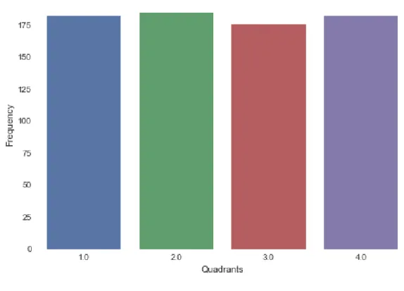
Furthermore, there is an imbalance of quadrant observations, genre observations and artist observations. Later, we will dive into the frequency of observations in genre and artist variables but for now we will focus on the quadrant imbalance. Quadrant 1 has 591 observations and Quadrant 3 has 681 observations. This contrasts with the 200 observations of Quadrant 2 and the 209 observations of Quadrant 4. This imbalance can lead to dubious results of the classifiers. We will dive into this in the implementation chapter.

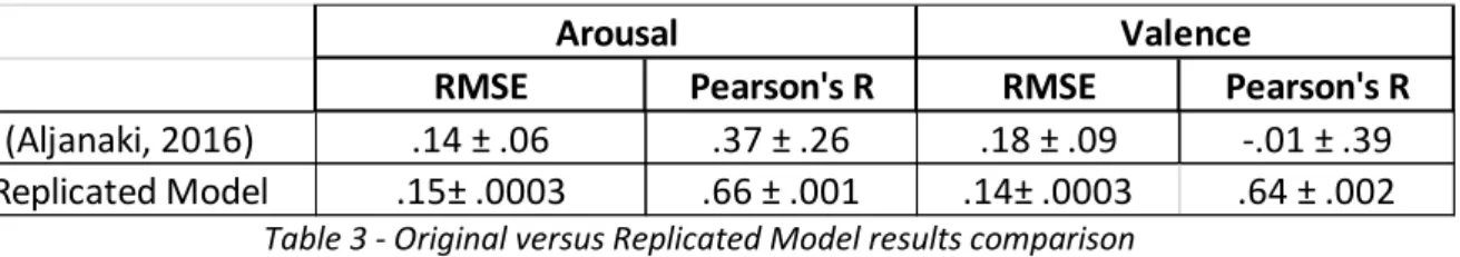
Lastly, to check if our audio features, which we will dive deeper later, are in the state-of-art level we replicated the baseline model that was presented by the researchers (Aljanaki, 2016). Note that the original model used dynamic annotations while we use static annotations. The model consists of a linear regression using 20 x 10-fold cross-validation to predict Arousal and Valence values in Rus-sel’s continuous emotion plane. Both dependent values were scaled to [0,1]. The audio features used in the paper differ from the ones we used, which leads to different results. The features used by the researchers were a combination of Kalman filter and low level audio features: MFCC’s, Zero-Crossing Rate, Spectral Flux, Roll off, Centroid and Spectral Crest Factors. The RMSE and Pearson’s R were cal-culated for each fold and the average and standard deviation of inter-fold RMSE and Pearson’s R were presented.

Table 3 - Original versus Replicated Model results comparison

On Table 3 it is possible to compare the results from both baseline models. In order to facilitate the interpretation, we will call the researchers model as original model and ours as replicated model. In the original model, both Valence and Arousal show a low average RMSE, which is a good indicator for model accuracy. In the replicated model, the RMSE for Arousal is similar and lower in Valence. The main strength of the replicated model when compared to the original one, is the Pearson’s R which is

RMSE Pearson's R RMSE Pearson's R

(Aljanaki, 2016) .14 ± .06 .37 ± .26 .18 ± .09 -.01 ± .39 Replicated Model .15± .0003 .66 ± .001 .14± .0003 .64 ± .002

22 0.66 for Arousal and 0.64 for Valence, while the original model has 0.37 and 0.18 respectively. This means that the correlation between the predicted values and the original values in the replicated model is higher which shows a better capacity for classification of this dataset. Furthermore, the stand-ard deviation values for both Arousal and Valence in the original model is high, showing symptoms that the classification model is volatile from fold to fold when compared with the replicated model.

Unfortunately, this was the only way to compare our model with other models which classified the whole DEAM dataset, but we have to keep in mind that static annotations usually show better results than dynamic annotations. With this analysis, we demonstrated that our audio features can keep with state-of-art research. As stated before, we will dive deeper into the detailed explanation of these audio features later.

AllMusic:

The AllMusic dataset consists in 1608 music clips each 30 second long. These songs were an-notated by 665 subjects regarding valence and arousal. It is the second largest dataset in MIR. Re-searchers opted for a dimensional framework where the listeners were asked to annotate perceived emotions on the valence-arousal space. The western music song list was selected from AllMusic and the respective 30-second sample was extracted from 7digital. The songs were annotated by 665 lis-teners from Amazon Mechanical Turk. To ensure annotation quality, it was required that the subjects were residents of the United States and had over 90% tasks done on Amazon Mechanical Turk. To measure inter-subject agreement on the annotations, the researchers calculated Krippendorff’s ⍺ which resulted in 0.31 on valence and 0.46 on arousal, which are considered fair agreement. (Chen et al., 2015). The main limitation of the dataset is the fact that it is partially public which makes impossible to extract new features from the songs. The annotations were made using listeners from Amazon Me-chanical Turk which can, as stated before, reduce the quality of the annotations. Lastly, most part of the annotations fall in the first quadrant of the arousal-valence space, which means there is a quadrant imbalance on the dataset.

Other Datasets:

23 The Soundtrack dataset, which consists of 110 film music excerpts of approximately 15 seconds each. The dataset is public and the annotations are based on perceived emotions of 116 non-musi-cians. In regards of the taxonomy, Eerola et al. (2011) used two different taxonomies to compare the results: half of the excerpts were representative of five discrete emotions (anger, fear, sadness, hap-piness and tenderness) and the other half were representative of three dimensions (valence, energy arousal and tension arousal). There was also released a set of 16 one-minute examples of emotions induced by music (Eerola & Vuoskoski, 2011). The main issues with this dataset is the small size and the fact that the excerpts are extracted from films which have considerable differences when com-pared to songs.

To conduct their research on semantic computing based of emotions on social tags, Saari & Eerola (2014) gathered a set of 600 randomly selected songs from Last.fm. The researchers used bal-anced random sampling to ensure that there was genre and emotion coverage. The sample also fa-vored tracks associated to many emotion tags and with many listeners. There was also a restriction of having only one song per artist. Rock and Pop were the most frequent genres on the dataset. To an-notate 15-second music clips of the songs, 59 participants were selected. Of these participants, 28 were musicians and 8 were trained professionals. The experiment was focused on emotions perceived and the listeners were asked to annotate the samples on bipolar terms: negative/positive, calm/ener-getic and relaxed/tense. To capture the continuous nature of emotion on songs, the results were con-verted to nine-step Linkert-scales (Saari & Eerola, 2014). One issue of the dataset is that the research-ers disclosed the annotations but not the samples and features. This means that future researchresearch-ers are not be able to replicate the results. Likewise, another main characteristic of the dataset, which makes unfeasible to our research, is the fact that the emotion annotations are continuous, while our focus is on the dominant emotion of the song. We could achieve the dominant emotion but it would create an additional layer of error to the annotation. Another limitation is the restriction to only on song per artist, which constraints any potential meaning of the variable Artist.

The Emotify dataset is composed of 400 one-minute song excerpts in four different genres (pop, classical, rock and electronic) collected through an online game named Emotify. The dataset is public and the annotations were made using GEMS scale (Geneva Emotional Music Scales), which is a taxonomy for induced emotions. Each annotator could skip the songs and switch musical genres be-cause, as stated by the researchers, induced emotions don’t occur in every song. The songs were split

24 genres, the lesser known songs had fewer annotations when compared with popular music (Aljanaki, Wiering, & Veltkamp, 2016).

MoodSwings public dataset has 240 fifteen-second music clips which were selected to repre-sent the four quadrants of the Arousal-Valence space. The annotations were made by participants online by listening to 30-second music clips and referring the dynamic position in the Arousal-Valence space. Later, the annotations were compared to other annotations developed using Mechanical Turk on the same music clips, which shown both sets of annotations were highly correlated (Schmidt & Kim, 2011). The small size is the main limitation of this dataset.

The Multi-modal MIREX-like emotion dataset was developed by Panda et al. (2013) by com-bining information from audio, lyrics and MIDI. The researchers used the MIREX framework to anno-tate 903 thirty-second audio clips, 764 lyrics and 193 MIDIs. The annotations were made resorting to the AllMusic database API (Panda, Malheiro, Rocha, Oliveira, & Paiva, 2013). This dataset is public but have some limitations. The first problem arises from the fact that it extracts the annotations from the AllMusic database, which have some quality problems since the annotation process is not clear (Malheiro, 2016). The only information is that these annotations are made by experts (Hu & Downie, 2007). Some of the excerpts were music intros or individuals talking. There is also the need to add an extra verification step when extracting labels from Last.fm. On their study, the verification step was made by 17 listeners, mainly students and researchers at the Music Technology Group (Laurier, 2011). On top of that, the MIREX framework has its own limitations, such as clusters overlapping semantically (Laurier et al., 2008).

2.3.4. MER Audio Frameworks Review

25 Marsyas

Marsyas or Music Analysis, Retrieval and Synthesis for Audio Signals, is an open-source soft-ware framework created by George Tzanetakis with the collaboration of students and researchers from around the world for audio processing with special application on the Music Information Retrieval field. One of the first frameworks in MIR, Marsyas is known for its computational efficiency, expected from a highly-optimized software written in C++. It has a solid user and developer base. Marsyas pro-vides the structure to develop full GUI applications through the native integration with Qt14. It is im-portant to note that the high number of features is due to the statistical measures calculated for each original feature. Some limitations are linked to the unsubstantial documentation, interface and syntax which require a steep learning curve, and difficult control of the audio processing networks.

MIR Toolbox

The MIR Toolbox is an integrated set of functions written in MATLAB for the extraction of mu-sical features such as rhythm, pitch, timbre and others. Designed in a modular way, the framework allows the decomposition of different algorithms into more elementary functions. The main advantage is the possibility of combining these modules into new features by using novel approaches (Lartillot & Toiviainen, 2007).

The framework can be scripted or used with an interface and offers capability of extraction of a considerable number of relevant low and high-level features to the field of MER (Panda & Paiva, 2011). The creators gave special attention to the ease of use of the software and syntax. The docu-mentation is pleasant when compared to other frameworks and there is the possibility of exporting and visualizing the extracted information. The main disadvantage is its reliance on

Math-Works’MATLAB and MathWorks’Signal Processing Toolbox on account of being commercial products

of this company. Contrary to Marsyas, MIR Toolbox does not offer real-time capabilities (Lartillot & Toiviainen, 2007).

jMIR

user-26 friendly. It is possible to create user scripts for batch processing and other features through the com-mand line interface. Other advantages include the higher number of audio features available. The fact that jMIR was built using Java makes it slower and heavier than other frameworks but also more port-able. Regarding the feature extraction process, jMIR provides components such as jAudio, jSymbolic and jLyrics.

jAudio is the component of jMIR which gives the ability of extracting features from audio files. A relevant aspect of this tool is the possibility of combining low-level features to build high-level fea-tures.

jSymbolic is used to extract high-level musical features from symbolic music representations such as MIDI files. It is commonly used by researchers in empirical musicology, music theory and MIR, mostly for the high-level musical features related to instrumentation, rhythm, dynamics, melody, chords, texture and pitch statistics.

Jlyrics is a set of software tools for mining lyrics from the web and extracting features from them.

LibRosa

LibRosa is an open-source Python package created by Brian McFee for processing audio and music signals. It was designed in a way that does not pose a steep learning curve, especially for re-searchers familiar to MATLAB. Functions are designed to be modular, providing users with the possi-bility of creating their own custom functions. The integration with the Python package Matplotlib pro-vides researchers with good visualizations of the rendered audio data (McFee et al., 2015). The ease of use and quality documentation are two other strengths of this software.

On the other hand, Librosa’s output will only allow users unstructured data in table format while other softwares such as MIR Toolbox and Marsyas can also produce ARFF files to ease the data mining task.

27

2.3.5. Audio Features Review

2.3.5.1. Intensity

Root-Mean-Square Energy (RMS):

Root-Mean-Square Energy measures the power of a signal over a window of time. It can also be used to understand the global energy of a signal 𝑥 by taking the root average of the square of the amplitude (RMS) (McEnnis, McKay, & Fujinaga, 2005), as shown below (Equation 2):

𝑥𝑅𝑀𝑆= √1_{𝑛 ∑ 𝑥}𝑖2 𝑛

𝑖=1

= √𝑥12+ 𝑥22_𝑛+ ⋯ + 𝑥𝑛2

Equation 2 – Root-Mean-Square Energy

Root-Mean-Square Derivative:

Indicates the change of signal power by representing the window-to-window change in RMS.

Root-Mean-Square Variability:

Gives the value of the standard deviation of the RMS on the last N windows.

Less-Than-Average Energy

In order to understand if the energy distribution remains constant throughout the signal, researchers can use the percentage of frames showing less-than-average energy, also known as low energy rate (Tzanetakis, 2002), as shown in Figure 6.

Figure 6 - Lower-than-average energy frames highlighted on Energy curve (Lartillot, 2013)

Fraction of Low Energy Frames:

28 previous windows in which the RMS is below the mean RMS, thus finding which are the windows whose signal is quiet relative to the rest of the signal section.

2.3.5.2. Rhythm

Indicates the rhythmic periodicity along auditory channels. The process of the estimation of these feature is based on two steps (Lartillot, 2009):

• First the spectrogram is computed on 23ms frames and half overlapping, then the Terhardt outer ear is modelled with Bark-band redistribution of energy and estimation of the masking effects. The amplitudes are then computed in a dB scale.

• After that, the FFT, which varies from 0 to 10 Hz, is computed for each Bark band. The final modulation of coefficients is based on a psychoacoustic model of the strength of the fluctuations. This results in a matrix filled with rhythmic periodicities of each Bark band.

Tempo:

Indicated by beats per minutes (BPM), measures the pace of a music piece and it is usually calculated by identifying the periodicities from the onset detection curve.

Strength of Strongest Beat:

Uses the beat histogram to identify the strongest beat and compare it to other beats (McKay, 2005).

Beat Sum:

Measured by the sum of all bins in the beat histogram, it is commonly used to assess the importance of regular beats on a given signal (McKay, 2005).

2.3.5.3. Timbre

29

Figure 7 - Attack Time detection (Lartillot, 2013)

Attack Slope:

Other measure used to indicate the attack phase, where the average slope of the whole attack phase is calculated since it starts until it reached the peak as shown in Figure 8.

Figure 8 - Attack Slope Example (Lartillot, 2013)

Zero Crossing Rate:

Consists on the count of times the waveform changes sign by crossing the horizontal axis, as shown on Figure 9. Commonly used to indicate the noisiness of a song.

Figure 9 - Zero Crossing Rate Waveform (Lartillot, 2013)

30 𝑍𝑡 =1_{2 ∑ |𝑠𝑖𝑔𝑛}(𝑥[𝑛]) − 𝑠𝑖𝑔𝑛(𝑥

𝑁

𝑛=1

[𝑛 − 1]|

Equation 3 – Zero Crossing Rate

Zero Crossing Derivative:

Estimation of the absolute value of the change from window-to-window in Zero Crossing, indicating noisiness and frequency.

Spectral Roll Off:

Commonly used to indicate the skew of the frequencies of a window, it consists on the fraction of the total energy in Hz that is below a given percentage threshold, as exemplified in Figure 10. Usually this threshold is set to 85% (Tzanetakis, 2002).

Figure 10 - Spectral Roll Off with frequency (Lartillot, 2013)

The Spectral Roll-Off, according to (Tzanetakis, 2002), is shown on Equation 4. 𝑹𝒕 stands for the frequency below which 85% of the magnitude distribution is condensed.

∑ 𝑀𝑡[𝑛] = 0.85 ∗ ∑ 𝑀𝑡[𝑛] 𝑁

𝑛=1 𝑅𝑡

𝑛=1

Equation 4 – Spectral Roll Off

High Frequency Energy:

31

Figure 11 - Spectral Roll Off using Percentage (Lartillot, 2013)

Spectral Flux:

Measures the distance between adjacent frames. Musical experiments showed that it is an important attribute for the listener's perception of musical instrument timbre (Tzanetakis, 2002).

Spectral Flux can be calculated as shown in Equation 5, where 𝑵𝒕[𝒏] , 𝑵𝒕−𝟏[𝒏] are the normalized magnitude of the Fourier transform at the current frame 𝒕, and the previous frame 𝒕 − 𝟏 (Tzanetakis, 2002).

𝐹𝑡 = ∑(𝑁𝑡[𝑛] − 𝑁𝑡−1[𝑛])2 𝑁

𝑛=1

Equation 5 – Spectral Flux

Mel-Frequency Cepstral Coefficients (MFCC):

Describe the spectral change of sound. The frequency bands are positioned on the Mel scale logarithmically. This approximates the human auditory response which is closer to reality than the linearly-spaced frequency bands.

To calculate MFCC, first we need to take the log-amplitude of the magnitude spectrum. Next, the FTT bins are grouped and smoother according to the Mel-scale. To eliminate the correlation between the resulting feature vectors, a Discrete Cosine Transform is used (Tzanetakis, 2002).

Sensory Dissonance (Roughness):

32

Figure 12 - Sensory Dissonance depending on frequency ratio (Lartillot, 2013)

Spectral Peaks Variability (Irregularity)

The degree of variation of the successive peaks of the spectrum. It can be calculated as shown in Equation 6, with the sum of the amplitude minus the mean of the preceding, current and next amplitude (Lartillot, 2009).

∑ |𝑎𝑘 −𝑎𝑘−1+ 𝑎₃𝑘+ 𝑎𝑘+1 𝑁−1

𝑘=2

|

Equation 6 – Spectral Peaks Variablity

Spectral Centroid:

Measuring the central shape, this feature indicates the “brightness” of the textures of the song. It can be calculated as following:

𝐶𝑡 =∑ 𝑀𝑡[𝑛] ∗ 𝑛 𝑁

𝑛=1

∑𝑁 𝑀𝑡[𝑛] 𝑛=1

Equation 7 – Spectral Centroid

In the Equation 7 , 𝑴𝒕[𝒏] represents the magnitude of the Fournier transform at frame 𝒕 and frequency bin 𝒏 (Tzanetakis, 2002).

Linear Prediction Reflection Coefficients:

33 Linear Spectral Pairs:

Represents linear prediction coefficients for transmission over a channel. This feature is not sensitive to quantization noise and it is stable, making them popular for speech coding.

Strongest Frequency via Spectral Centroid:

This feature is an estimation of the strongest frequency component of a signal (Hz), by using the spectral centroid (McKay, 2005).

Spectral Crest Factor:

Known also as peak-to-average ratio, this feature is a measure of a waveform, calculated from the peak amplitude divided by the RMS value of the given waveform as shown in the following formula (Equation 8):

𝐶 =|𝑥|𝑝𝑒𝑎𝑘_{𝑥𝑟𝑚𝑠}

Equation 8 –Spectral Crest Factor

Spectral Flatness Measure:

Characterizes an audio spectrum: if the graph of the spectrum appears flat and smooth, the Spectral Flatness Measure (SFM) is probably high. This happens because a high SFM means that a spectrum has a similar amount of energy across all spectral bands, while a low SFM describes a spectrum where the power is condensed in a small number of bands.

It can be calculated by dividing the mean of the geometric power spectrum by the arithmetic mean of the power spectrum (Equation 9). In the equation, 𝒙(𝒏) represents the magnitude of bin number 𝒏:

𝑆𝐹𝑀 = √∏ 𝑥(𝑛)

𝑁−1 𝑛=0 𝑁

∑𝑁=1𝑥(𝑛) 𝑛=0

𝑁

Equation 9 –Spectral Flatness Measure

Inharmonicity:

34

Figure 13 - Fundamental frequency (f0) and respective multiples (Lartillot, 2013)

2.3.5.4. Pitch

Pitch:

Indicates the perceived fundamental frequency of a given sound. Along with loudness and timbre, it is one of the three major auditory sound attributes. It represents the fundamental frequency of a monophonic sound signal (Tzanetakis, 2002).

Strongest Frequency via FFT maximum:

Estimation of the strongest frequency component in a given signal (Hz) found via FFT bin with the highest power (McKay, 2005).

2.3.5.5. Tonality

Key:

Estimation of tonal centre positions and their respective clarity (McKay, 2005).

Mode:

Indicates the difference between major and minor keys of a given piece.

Tonal Centroid:

35

Figure 14 - Tonal Centroid for a major triad is shown at point A (Lee, 2008)

Harmonic Change Detection Function:

Represents the flux of the tonal centroid (Lartillot, 2009).

2.3.5.6. Musical Features

Divided in two distinct categories, rhythmic and pitch content, this features are based on mu-sical content and information extracted from previous mentioned features (Tzanetakis, 2002).

Rhythmic Features – calculated via Beat Histograms (BH) of a song:

• A0, A1: relative amplitude of the first (A0) and second (A1) histogram peak; • RA: ratio of the amplitude of the second peak and the amplitude of the first peak; • P1, P2: period of the first (P1) and second (P2) peaks in Beats per Minute;

• SUM: sum of the histogram, refers to the beat strength.

Pitch Features – calculated via Folded Pitch (FPH) and Unfolded Pitch (UPH) Histograms of a song: • FA0: amplitude of the maximum peak of the FPH, indicates the most dominant pitch class of a

song;

• UP0: period of the maximum peak of the UPH, it refers to the octave range of the dominant musical pitch of a given song;

36 • IPO1: pitch interval between the two most prominent peaks of the FPH, referring to the main

tonal interval relation;

37

3.

IMPLEMENTATION

3.1. Pre-processing the Dataset

We will use the DEAM dataset, which is composed of 1802 songs (1744 samples of 45s each and 58 full-length songs). As mentioned previously, the excerpts have a sampling frequency of 44100Hz and were annotated according to the continuous emotion taxonomy representation of Russel’s model of Valence-Arousal.

From the original dataset, 9 songs were removed because there was no annotation associated with this samples. This represents 0.49% of the DEAM dataset.

We transformed the numerical values of the Russel’s model of Valence-Arousal into four quadrants, which is the Categorical version of this emotion taxonomy (Malheiro, Oliveira, Gomes, & Paiva, 2016). We will dive into the process later. Since our dependent variable, Quadrants, is not numerical after the before mentioned transformation, this is considered a Classification Problem.

We used Python to implement most of the project, from Data Pre-processing until Data Visualization. There were other tools used that will be mentioned when necessary.

Our variables can be divided into 4 groups: quadrants annotated, audio features, genre and artist. Quadrants annotated is the dependent variable while the other groups consist of independent variables. We will dive into each one of these groups and explain which transformations were done. In the end, we will present the final dataset used to train the machine learning algorithms.

3.1.1. Quadrants

Our dependent variable, Quadrants, consists of static annotations on the dataset songs. The annotations were performed in a 9-point scale for Valence and Arousal. The emotion taxonomy followed by the researchers was a numerical representation of Russel’s model of Valence-Arousal. The minimum was 1 and the maximum was 9 for Valence and Arousal and the final annotations for each song was the average of all the annotators rating. Each song was annotated by a minimum of 5 listeners.

38

Figure 15 - Russel’s Circumplex Model (Y.-H. Yang et al., 2008)

We did not round the numbers either up or down. To avoid ambiguity, the 108 songs that were placed on top of one of the axis were removed, which represents 6.02% of the total dataset.