Global warming projections derived from an observation-based minimal model

(1)

www.earth-syst-dynam.net/7/51/2016/ doi:10.5194/esd-7-51-2016

Global warming projections derived from an

observation-based minimal model

K. Rypdal

Department of Mathematics and Statistics, UiT The Arctic University of Norway, Tromsø, Norway

Correspondence to:K. Rypdal (kristoffer.rypdal@uit.no)

Received: 24 August 2015 – Published in Earth Syst. Dynam. Discuss.: 18 September 2015 Revised: 7 January 2016 – Accepted: 10 January 2016 – Published: 29 January 2016

Abstract. A simple conceptual model for the global mean surface temperature (GMST) response to CO2 emis-sions is presented and analysed. It consists of linear long-memory models for the GMST anomaly response1T

to radiative forcing and the atmospheric CO2-concentration response1C to emission rate. The responses are connected by the standard logarithmic relation between CO2concentration and its radiative forcing. The model depends on two sensitivity parameters, αT andαC, and two “inertia parameters,” the memory exponentsβT

andβC. Based on observation data, and constrained by results from the Climate Model Intercomparison Project Phase 5 (CMIP5), the likely values and range of these parameters are estimated, and projections of future warm-ing for the parameters in this range are computed for various idealised, but instructive, emission scenarios. It is concluded that delays in the initiation of an effective global emission reduction regime is the single most im-portant factor that influences the magnitude of global warming over the next 2 centuries. The most imim-portant aspect of this study is the simplicity and transparency of the conceptual model, which makes it a useful tool for communicating the issue to non-climatologists, students, policy makers, and the general public.

1 Introduction

In spite of five comprehensive reports from the Intergovern-mental Panel on Climate Change (IPCC), the perception of the threat of global warming to society remains highly di-verse among the general public, decision makers, and the scientific community at large. This is in stark contrast to the general opinion among those who define themselves as climate scientists, where some studies suggest that as much as 97 % recognise human activity as a main driver of global warming over the last century (Anderegg et al., 2010; Cook et al., 2013). What distinguishes the climate science com-munity from other scientists is the strong reliance among climate scientists on complex earth system models (ESMs), that is, on atmospheric–ocean general circulation models (AOGCMs) coupled to models that include biogeochemistry and cryosphere dynamics. The general skepticism concern-ing this “model science” is not hard to understand. Mod-els are complex beyond comprehension, different modMod-els are not independent but consist of many common modules, and parametrisations are empirical to an extent that makes it

le-gitimate to question whether models are “massaged” to fit observations. The important point here is not whether this perception of climate modelling is correct or fair but that the skepticism exists and in many cases cannot be discarded as irrational.

The latest IPCC report from Work Group I on the climate system (IPCC AR5 WG1, 2013) contains a summary for policy makers that describes findings from observations and model studies, which many physical scientists find uncon-vincing and which is not a very easy read for the general pub-lic. The unconvincing part is the above-mentioned excessive reliance on complex computer models. Most scientists want to understand and to be convinced by simple fundamental principles matched against clear-cut observations. Decision makers and the informed layman want to see simple, clear alternatives for the future, not a myriad of incomprehensi-ble scenarios labelled by acronyms that carry no meaning to non-experts.

(2)

the Co-Chair of Work Group I alongside the IPCC AR5 re-port, intended to demonstrate that as mitigation is delayed, climate targets formulated in international agreements be-come unattainable. The results were based on the physi-cal assumption of a linear relationship between the cumu-lated carbon emissions and peak global warming in scenarios where the cumulative emission is bounded. This relationship, and the constant of proportionality, were justified empirically from numerical experiments performed on a large number of ESMs which incorporate the global carbon cycle (Allen et al., 2009; Matthews et al., 2009). Some readers, however, will find it unsatisfactory that they have to “believe” the mod-els in order to accept the conclusion of the paper. As a for-mer plasma physicist, who only relatively recently has taken up research in earth system dynamics and climate science, I am often confronted with questions from former colleagues of the following type: “For half a century we have tried to model the transport properties of a magnetically confined plasma for controlled thermonuclear fusion, and we still have not succeeded very well, even though the physical system is infinitely simpler than the climate. Why do you think these horrendously complex climate models perform any better?”. A major motivation for the present paper is to find ways to communicate with, and gain support from, the scientists who ask such questions. I do this by deriving results simi-lar to those obtained in Stocker (2013) in a more transpar-ent manner and without resorting to complex ESMs as the primary justification. The underlying assumptions are justi-fied from observations, although supporting evidence from AOGCMs is also discussed. The conceptual models of the temperature and atmospheric carbon response are linear and simple enough to be understood by anyone with some back-ground in elementary calculus and ordinary differential equa-tions. The scenarios explored are idealised and the results presented in figures that should be comprehensible for read-ers without training in mathematics or physical sciences.

Section 2 describes and justifies the conceptual model. Section 3 presents projections for atmospheric CO2 concen-tration and global mean surface temperature (GMST) for some idealised CO2 emission scenarios: one which is very close to the “business as usual” Representative Concentra-tion Pathway 8.5 (RCP8.5) scenario employed by the IPCC, and other scenarios which represent systematic emission re-duction initiated at different times in the future. This section also discusses policy implications that may follow from these projections, and Sect. 4 summarises and concludes the paper. Six appendices elaborate on the physical interpretation and justification of the minimal model and on some mathemat-ical aspects that may appear as paradoxes. This material is placed in appendices in order to avoid the interruption of the logical flow that leads to the main results. The Supplement contains data files and a well-documentedMathematica note-book with routines that allow readers to replicate and extend all results presented in the paper.

2 The conceptual model

A closed model for the evolution of the global mean sur-face temperature (GMST) could consist of (i) a model for the GMST anomaly response1T(t) to radiative forcingF(t), (ii) a model for the evolution of1C(t), given the CO2 emis-sion history R(t), and (iii) a well-established constitutive relation betweenF(t) and1C(t). This paper proposes ex-tremely simple, linear models for the GMST response (i) and the CO2 concentration response (ii). Each depends on two parameters characterising the strength and the inertia (mem-ory) of the response. In order to keep the model sufficiently simple for a reader to be able to trace the connection between driver and response and the effect of variation of model pa-rameters, major simplifying assumptions are made. One is to neglect all radiative forcing other than CO2. Although the main reason for this is to maintain simplicity, it is justified by forcing estimates that conclude that the non-CO2 contri-butions tend to cancel out over the industrial period (IPCC AR5 WG1, 2013). Other important simplifications are lin-earity and stationarity.

2.1 Linearity

Global temperature has been found to respond quite linearly to forcing in general circulation models (Meehl et al., 2004), and as long as the climate system is far from a major tip-ping point, this linearity may also pertain to the response of atmospheric CO2content to emissions. The effect of space– time non-linearity is important primarily in variability on a scale smaller than the global scale. On the global scale the response function has an approximate power-law form that makes the system respond by a scale-invariant stochastic pro-cess to a white-noise driver. This scale invariance is charac-terised by a spectral exponentβ, which gives rise to a power-law tail in the response functionG(s)∼sβ/2−1, wheres is the time following an impulse in the forcing. The physical interpretation of such a response is that the climate system consists of a number of different interacting subsystems with different response times. There will be a maximum response time and hence there will be a cut-off of the power-law tail in the response function forslarger than this maximal time constant. The justification, interpretation and implication of this picture is further discussed in the appendices.

2.2 Stationarity

(3)

Dansgaard–Oeschger events during the last ice age (Bender, 2013). During the present interglacial period, the Holocene, there was a similar tipping event about 8.2 kyr ago. These events are believed to be associated with a sudden influx of freshwater into the North Atlantic from the North American Laurentide ice sheet and related changes in the overturning ocean circulation. A number of potential tipping elements have been identified associated with global warming in the present Holocene climate (Lenton et al., 2013). Among these are the complete disappearance of the Arctic sea ice, run-away melting of the Greenland and West Antarctic ice sheets, a radical change in the Atlantic thermohaline ocean circula-tion and the El Niño–Southern Oscillacircula-tion, shifts in the In-dian and the western African monsoons, and dieback of the Amazon and the boreal forests. Transitions associated with tipping elements of these types can change the global tem-perature response as well as the carbon-cycle response sig-nificantly. Even in the absence of tipping points, the station-arity assumption may be particularly wrong for the CO2 con-centration, where, e.g., saturation effects in the ocean mixed layer and the land biosphere may reduce fluxes in a future cli-mate. It also neglects the coupling between sea surface tem-perature and the CO2 flux, which will reduce the flux into the ocean in a warmer climate. However, experiments with carbon-cycle models subject to sudden CO2injections into the atmosphere indicate that the response in the CO2 concen-tration can be described by a power-law response function. This response is not stationary in the sense that it will be the same for a new carbon release in a future climate, but it may give an adequate description of the response to the present global warming event. Further details are given in Sects. 2.3 and 2.4 and in the appendices.

2.3 The temperature response

The simplest physics-based model of the GMST response is the zero-dimensional, linearised energy balance model (EBM):

d

dt1T = −

1

τT

1T+ S

τT

F. (1)

Here,τT is the time constant for the relaxation of the

tem-perature anomaly andSis the climate sensitivity. The model is often denoted the Budyko–Sellers model and was first pro-posed by Budyko (1969) and Sellers (1969). A simple deriva-tion can be found in Rypdal (2012), where it is also pointed out that it is impossible to find a single time constant that de-scribes adequately the response to forcing on all timescales. The reduction to a linear model from the nonlinear EBM with the full Stefan–Boltzmann radiation law is found in Ap-pendix E. This model is not only used for reproducing the global temperature to known (deterministic) forcing but can also be formulated as a stochastic differential equation by introducing a noise component to the forcing F(t), repre-senting the stochastic energy flux from atmospheric weather

systems to the ocean and land surface (Rypdal and Rypdal, 2014). The solution to this equation can be written as a con-volution integral

1T(t)= t

Z

0

GT(t−t′)F(t′) dt′, (2)

with an exponential response function

GT(t)=(S/τT) exp(−t /τT). (3)

The temperature response to a purely stochastic forcing, i. e., F(t) is represented as Gaussian white noise and is an Ornstein–Uhlenbeck stochastic process. In discrete time, this corresponds to a first-order autoregressive (AR(1)) process. If Eq. (1) provides an adequate description, withF(t) sepa-rated into a deterministic and a white-noise component, then the residual obtained after subtracting the deterministic re-sponse from the observed annual GMST record should be a realisation of an AR(1) process. The time constant and the climate sensitivity can be determined by a maximum-likelihood estimation, and in Rypdal and Rypdal (2014), they were estimated to beτ≈4.3 years and S≈0.32 km2W−1_. However, the sensitivity obtained is lower than that obtained from climate models, the fast response to volcanic eruptions is higher than in the observed record, and the residual does not conform well with an AR(1) process. Rypdal and Rypdal (2014) demonstrated that the residual is better described by a model for persistent, fractional Gaussian noise (fGn). Such a noise can be produced by Eq. (2) if the exponential response function is replaced by a power-law function

GT(t)=αTtβT/2−1, (4)

where the memory exponentβT is in the interval 0< βT <1.

It can be shown that this process has a power spectral den-sity of the form∼f−βT_{, where}_f _{is the frequency (Beran,}

1994). Hence,βT =0 corresponds to white noise, while

in-creasingβT signifies increasing degree of memory (or

persis-tence) in the process. In this response model it replaces the time constantτT of the simple EBM. The parameterαT

re-places the climate sensitivityS. In Rypdal and Rypdal (2014) the magnitude of the parametersαT andβT were estimated

from the instrumental GMST record, revealing rather strong persistence (βT ≈ 0.75). Similar values were also found in

(4)

��

1900 1950 2000 2050 2100 2150 2200 0 2 4 6 8 10 12 Year Te m p e ra tu re ( K ) GMST projections

1900 1950 2000 2050 2100 2150 2200 0 5 10 15 Year Fo rc in g ( W m -2 )

Stabilised forcing scenarios

1900 1950 2000 2050 2100 2150 2200 0 2 4 6 8 10 12 Year Te m p e ra tu re ( K )

GMST with stabilised forcing

1900 1950 2000 2050 2100 2150 2200 0 2 4 6 8 10 12 Year Te m p e ra tu re ( K )

GMST with stabilised forcing

βT=0.35 βT=0.75

(a)

(c)

(b)

(d)

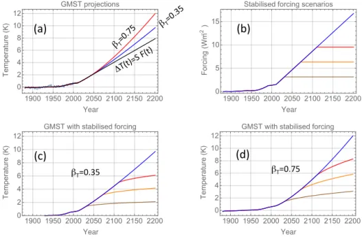
Figure 1.Panel(a): light blue curve is the instrumental GMST for 1880–2010 AD. Black curve is the instantaneous response to the linearly

extrapolated forcing scenario shown in panel(b). Blue curve is the response according to the model Eq. (2) withβT =0.35, and the red curve

is the response withβT =0.75. Panel(b): the straight sloping line is a linearly projected forcing to 2200 AD with the same mean growth

rate as the RCP8.5 scenario in the period 2010–2100 AD. The horizontal line is the stabilisation of this forcing in 2030 AD, the horizontal orange line in 2070 AD, and the red horizontal line in 2110 AD. Panel(c): GMST responses to the forcing scenarios in(b)withβT =0.35.

Colours correspond to those in(b). Panel(d): same as in(c)but withβT =0.75.

to transient simulations of AOGCMs following an abrupt in-crease in CO2forcing, and the two time constants estimated from these data were typically 1–2 years and 1–2 centuries. In Rypdal et al. (2015), it was shown that a power-law re-sponse provides an even better fit to the tail of the tran-sient AOGCM solutions, but the memory exponent is lower (βT ≈ 0.35) than that found from the residuals in

observa-tions and AOGCM simulaobserva-tions with historical forcing. One way of reconciling these conflicting results is to assume that the forcing noise is not white but rather a persistent noise, which makes a contribution to theβT observed in the

resid-uals. Details are shown in Appendix D. On the other hand, it will be shown in Sect. 3 that the Coupled Model Intercompar-ison Project Phase 5 (CMIP5) in the RCP8.5 CO2 concentra-tion scenario yields results consistent withβT =0.75. Since

this implies some uncertainty with respect to the correct value ofβT for the temperature response, I shall present

pro-jections for the values βT =0.35 andβT =0.75 in Sect. 3,

assuming thatβT is likely within this interval.

The significance of the inertia, or long-range memory (LRM), in the temperature response for GMST projections is illustrated in Fig. 1. Panel a shows the estimated GMST response to the forcing scenario consisting of the anthro-pogenic forcing in the period 1880–2010 as presented in Hansen et al. (2011), linearly projected to 2200 AD with the same mean growth rate as the RCP8.5 scenario in the period 2010–2100 AD (Meinshausen et al., 2011); it is shown as the

blue curve in Fig. 1b. The blue and red curves in Fig. 1a are the responses according to the power-law response models withβT =0.35, andβT =0.75. The projection for an instant

response (τT →0, leading to1T(t)→S F(t)) is also shown

as the limit of zero inertia. Also shown as a light blue curve is the instrumental GMST record as given by Brohan et al. (2006). These projections have been obtained by computing the integralR₀tαT(t−t′)(βT/2−1)F(t′) dt′ with the specified βT and then estimating αT by regressing to the observed

GMST record for the period 1880–2010 AD. The climate sensitivity S for the instantaneous response has also been found by regressingSF(t) to the instrumental data, and is found to beS ≈0.48 km2_W−1_{, which corresponds to 1.8 K} for a doubling of CO2 concentration. The rising warming projected for increasingβT is a manifestation of the thermal

inertia in parts of the climate system with high heat capacity that exchange heat with the surface, and it makes the surface temperature respond more slowly. The higher surface warm-ing in the distant future due to this inertia is a manifestation of the warming in the pipeline (Hansen et al., 2011; Rypdal, 2012).

(5)

23rd century. This figure also shows some idealised scenarios where the BAU is modified by mitigation action. One possi-ble type of action is the sudden reduction in emission that will stabilise the forcing at the level of the time of action. In the real world such an action from one year to another is not possible, but it may be considered an approximation of a certain annual reduction over a period of 1 decade. For instance, a 40 % emission reduction can be achieved by an annual emission reduction of 5 % over 1 decade. In Fig. 1b forcing scenarios for this type of mitigation action are illus-trated assuming the onset of action in three different years: 2030, 2070, and 2110 AD. The year 2030 gives the world 15 years to prepare the action. Year 2070 leaves the problem to those who are born today, i.e. to the next generation. Year 2110 leaves it to unborn generations.

The GMST projections for these scenarios are shown in Fig. 1c, d for the lower and higher memory exponents

βT. Under the low-inertia assumption in the temperature

response (βT =0.35), the unmitigated forcing scenario in

Fig. 1a yields approximately 2◦_{C of warming every 40 years}

throughout the 21st century and an even higher rate of warm-ing in the 22nd century. After stabilisation of the atmo-spheric CO2concentration, the temperature will continue to rise about 1◦_{C by the year 2200 AD, independently of when}

this stabilisation takes place. This 1◦_{C of additional}

warm-ing is the warmwarm-ing in the pipeline. Under the high-inertia assumption (βT =0.75), the warming rate is approximately

30 % higher, and the warming in the pipeline is about a 100 % higher. The high-inertia projection with mitigation action in 2110 AD is very close to the multimodel mean RCP8.5 pro-jection (Meinshausen et al., 2011), suggesting some con-sistency between this simple global temperature response model and the models employed by the IPCC in the CMIP5 project.

Figure 1c, d suggest that the 2◦_{C target is unlikely to be}

attained by rapid stabilisation of atmospheric CO2 concen-tration if this action is started later than 2030 AD. If radical action is postponed until the GMST has passed the 2◦_{C limit,}

it is likely that the global temperature will exceed 3◦_{C by}

2100 AD, and if action is postponed until the end of this cen-tury our descendants may experience a world that is 5–8◦_C

warmer than before industrialisation.

2.4 The atmospheric CO₂response

The dominant driver of climate change throughout the 20th century and beyond is anthropogenic radiative forcing, and in the 21st century, CO2forcing is expected to be the main an-thropogenic driver. However, while AOGCMs traditionally have been driven by prescribing the atmospheric CO2 con-centration, the policy-relevant quantity is the CO2emission rate. The main factor that determines future CO2forcing in a given emission scenario is the rate at which CO2is washed out of the atmosphere. This is where the carbon-cycle models incorporated into the ESMs become important. The model

uncertainty is high, but the models suggest the existence of a hierarchy of timescales, just as we have found in the tem-perature response (Joos et al., 2011). This hierarchy is not immediately apparent from the instrumental data records, but there is some indirect evidence, as will be demonstrated be-low. However, let us first consider a primitive model with only one response timescale, analogous to the simple EBM given by Eq. (1) for the surface temperature. In this model we assume that the carbon flux out of the atmosphere is pro-portional to the anomaly1C of atmospheric carbon content relative to the preindustrial concentrationC0. This assump-tion follows from a Taylor expansion to first order of the car-bon flux I(1C)=(1/τc)1C+. . .around the preindustrial equilibriumI(C0)=0. The primitive equation for this per-turbation is then

d

dt1C= −

1

τC

1C+R, (5)

whereτCis the time constant for the relaxation of CO2 con-centration to the preindustrial equilibrium. A first-order es-timate ofτCcan be made from the estimates of the global carbon budget (Le Quéré et al., 2014). The annual carbon emission in the period 1960–2010 grew almost linearly from 4 Gt C yr−1_{to 11 Gt C yr}−1_{. We can solve Eq. (5) for this} pe-riod withR= [4+(7/50)]tGt C yr−1_{in terms of}_τ

Cand the initial atmospheric carbon inventory anomaly,1C1960. The conversion factor from concentration in part per million to gi-gatons of carbon in total carbon content is 2.12 (Le Quéré et al., 2014), which yields1C1960=(315–280)×2.12≈74 Gt C if we assume a CO2concentration of 315 ppm in 1960 and a preindustrial concentration of 280 ppm. The preindustrial carbon content, corresponding to 280 ppm, wasC0≈594 Gt C. This solution reproduces very well the observed evolution of the atmospheric CO2content in this period if one chooses

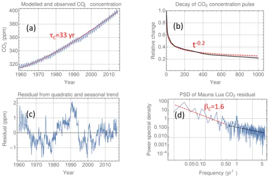
τC=33 years, as shown in Fig. 2a, and suggests that1C(t) is described by the response function

1GC(t)=(r/τC) exp[−t /τC]. (6)

A calibration factorrhas been introduced here because this response function is certainly too simplistic. For instance, Taylor expansion to first order does not take into account the saturation of carbon flux into the ocean, which will invoke a much longer response time governed by biogeochemical pro-cesses of the transport of carbon from the mixed layer into the deep ocean. If we fixτ_cat value higher than 33 years,r

can be estimated by a simple, linear regression to the historic CO2 concentration record. For τC=33 years such regres-sion yields of courser ≈1 but forτC≥ 300 years, it yields

(6)

��

1960 1970 1980 1990 2000 2010 320

340 360 380 400

Year

CO

2

(ppm)

Modelled and observed CO concentration2

0 200 400 600 800 1000 0.2

0.4 0.6 0.8 1.0

Year

Relat

ive

change

Decay of CO2concentration pulse

1960 1970 1980 1990 2000 2010

-1 0 1 2

Year

Residual

(ppm)

Residual from quadratic and seasonal trend

0.05 0.10 0.50 1 5 10-4

0.001 0.010 0.100 1 10 100

Frequency (yr )- 1

P

ower

spect

ral

densit

y

PSD of Mauna Lua CO2residual τ_C=33 yr

t

‐0.2

βC=1.6

(a)

(c)

(b)

(d)

Figure 2.Panel(a): blue curve shows the atmospheric CO₂concentration as measured by the Mauna Loa observatory. The red curve is

the concentration computed from Eq. (5) withτ_C=33 years,1C₁₉₆₀=74 Gt C (corresponding to an anomaly of 315–280=35 ppm), and C0=594 Gt C (corresponding to 280 ppm). Panel(b): black curve is the multimodel mean CO2response to a pulse of emitted CO2as given in Joos et al. (2011). The red, dashed curve is a least-square fit of a function of the formα_CtβC/2−1_{with the estimated}_β_C_≈₁_._{6. Panel}_(c):

the residual Mauna Loa signal after subtracting the quadratic polynomial and seasonal trends. Panel(d): the power spectral density of the residual in(c)estimated by the periodogram presented in a log–log plot. The black, dashed line has negative slopeβ_C=0.85, and the red, dashed line hasβC=1.6.

may suggest a hierarchy of timescales for the CO2 concen-tration response. The large model comparison study of Joos et al. (2011) reveals a non-exponential tail in the response to a pulse of emitted CO2. Figure 2b shows that the multimodel mean is very well approximated by a power law of the form

G_C(t)=α_CtβC/2−1_, ₍₇₎

withβC≈ 1.6. This power-law response suggests the sim-ple, linear response model

1C(t)= t

Z

0

G_C(t−t′)R(t′) dt′, (8)

where the emission rateR(t) may contain a stochastic con-tribution, giving rise to a stochastic component to1C. This stochastic component of1Cis shown in Fig. 2c, as the resid-ual obtained after subtracting a quadratic, polynomial fit to the Mauna Loa record (the anthropogenic trend) and the sea-sonal variation. The power spectral density of this residual is shown in Fig. 2c and indicates that the spectrum is con-sistent with a power law with a spectral indexβC ≈1.6 on timescales longer than a few years. The short duration of the record precludesaccurateestimates ofβCfrom the spectrum, but it lends some support to the power-law response model with a memory exponent in the range 1< βC<2.

2.5 The constitutive relation

A simple relation between CO2concentration anomaly and its radiative forcing is (Myhre et al., 1998)

F =5.35 ln(1+1C/C0) Wm−2. (9)

Given an emission scenarioR(t), Eq. (8) can be used to com-pute1C(t), and from Eq. (9) one obtainsF(t). Finally, this forcing is applied in Eq. (2) to compute1T(t).

3 Projections

3.1 Emission scenarios

(7)

��

1900 1950 2000 2050 2100 2150 2200 0

20 40 60 80

Year

Carbon

emission

rat

e

(

G

tC

) CO2emission scenarios

Figure 3.Blue curve is carbon emission rateR(t) scenario obtained

by fitting the exponentialS₀exp(gt) to the emission rate 4 Gt C yr−1 in 1960 and 11 Gt C yr−1in 2010 AD. The solid, brown, orange, and red curves are the subsequentR(t) after initiation of a 1 % re-duction in the emission rate per year. The dashed curves are the corresponding rates with a 5 % reduction per year.

of the world economy (Elzen et al., 2007). The scenarios are similar to those considered by Stocker (2013), although they are prescribed from 1880 AD, not from the present day. This is important for the response models employed here, since inertia (long-memory) effects from the historical period of global emissions and warming influence the future projec-tions.

3.2 Projections of CO₂concentration

Atmospheric CO2 concentrations 1C(t) for the emission scenarios described in Fig. 3 are shown in Fig. 4. They are computed from Eq. (8), using the emission scenarios of Fig. 3 and subsequently estimating r by regressing to the historic 1C(t) record. Figure 4a shows the corresponding concentration scenarios estimated from the exponential re-sponse kernel withτc=33 years. Few climate scientists be-lieve that atmospheric, anthropogenic CO2is eliminated as fast as this, but it is interesting to examine, since this is still claimed by some global warming skeptics (Solomon, 2008). In Fig. 4b and d the same scenarios are shown, assuming

τc=300 years andτc= ∞, respectively. Herer ≈0.5, i.e. 50 % of the emitted CO2, is immediately removed from the atmosphere and the rest decays exponentially with e-folding timeτC. Figure 4c employs the power-law response kernel withβC=1.6. Figure 4b and c are almost identical, indicat-ing that the immediate removal of half of the emitted CO2, followed by an exponential decay with τ_C=300 years, has almost the same effect as a long-memory (power-law) re-sponse withβC=1.6.

The unmitigated concentration scenarios (blue curves) are almost the same in all models and are very similar to the RCP8.5 scenario up to 2100 AD. This is because the calibra-tion factor r adjusts the scenario to fit the historic record. However, the evolution after mitigation action has started varies considerably between the models. The overly opti-mistic model in Fig. 4a, where τC=33 years, predicts that

the concentration starts declining a few decades after emis-sion reduction has started, whereas concentration continues to rise beyond 2200 AD in the 1 % reduction scenarios. The scenarios corresponding to the red solid curves in Fig. 4b and c correspond closely to the full RCP8.5 scenario.

3.3 Projections of the GMST

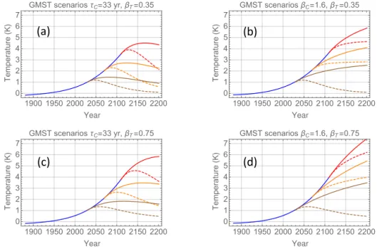
The forcingF(t) for the various concentration scenarios is computed from Eq. (9) and inserted into Eq. (2) to obtain the temperature evolution. Figure 5 shows results for the concen-tration scenarios obtained from the exponential CO2 concen-tration model withτC=33 years and the power-law model withβC=1.6, considering these to represent low- and high-inertia ends of the CO2 response. For each of these cases, low- and high-inertia ends (βT =0.35 andβT =0.75) of the

GMST response are presented in the figure.

The projections for the high-inertia combinationβC=1.6,

βT =0.75 shown in Fig. 5d is the one that is most

consis-tent with multimodel CMIP5 projections in the RCP8.5 sce-nario. As mentioned in Sect. 3.2, the red curve in Fig. 4c is close to the RCP8.5 CO2 concentration pathway, and the corresponding GMST response shown by the red curve in Fig. 5d is close to the multimodel mean GMST response given in Fig. 6 of Meinshausen et al. (2011). The high-end inertia (βT =0.75) for GMST response is also more

con-sistent with the analysis of instrumental records and multi-proxy reconstructions of GMST (Rypdal et al., 2015) and millennium-long simulations of intermediate and high com-plexity (Østvand et al., 2014). The high-end inertia for the CO2response is also more consistent with complex carbon-cycle models, and the long-memory nature of the residual Mauna Loa record, as shown in Fig. 2d.

3.4 Policy implications

(8)

ob-��

1900 1950 2000 2050 2100 2150 2200 0 500 1000 1500 2000 Year CO 2 concent rat ion ( ppm

) CO2concentration scenarios,τC=33 yr

) CO2concentration scenarios,τC=300 yr

) CO2concentration scenarios,βC=1.6

) CO2concentration scenarios,τC=∞

(a)

(b)

(c)

(d)

Figure 4.Projections of CO2concentration under the emission scenarios in Fig. 3 using the modelling explained in Sect. 2. The colours

correspond to those in Fig. 3. Panel(a):τ_C=33 years; panel(b):τ_C=300 years; panel(c):β_C=1.6; panel(d):τ_C= ∞.

��

1900 1950 2000 2050 2100 2150 2200 0 1 2 3 4 5 6 7 Year Te m p e ra tu re ( K )

GMST scenariosτC=33 yr,βT=0.35

GMST scenariosβC=1.6,βT=0.35

GMST scenariosτC=33 yr,βT=0.75

GMST scenariosβC=1.6,βT=0.75

(a)

(b)

(c)

(d)

Figure 5.The evolution of the GMST for the CO2concentration scenarios shown in Fig. 4a and c. Panel(a):τC=33 years andβT =0.35;

panel(b):βC=1.6 andβT =0.35; panel(c):τC=33 years andβT =0.75; panel(d):βC=1.6 andβT =0.75.

served by comparing Fig. 5a and d. The effect of emission reduction is considerably greater under the optimistic low-inertia assumptions, but in all circumstances, delayed miti-gation action increases the GMST in 2200 AD by 1–2◦_{C for}

every 40 years of delay.

One implication from this observation is that the global warming optimists have little reason for their optimism, since even the projections in Fig. 5a imply that the 2◦_{C climate}

tar-get will not be attained unless a radical and consistent emis-sion reduction regime is initiated within a few decades from now. If this mitigation regime is delayed and initiated one generation later, even the optimistic projections indicate that the temperature will peak close to 3◦C during the next cen-tury, and postponing reduction for yet another generation will let the temperature rise beyond 4◦_{C. If emission reductions}

(9)

temperature will not change much, but the temperature will come down faster after action has been initiated.

Under the more pessimistic, and presumably more realis-tic, circumstances presented in Fig. 5b and d, the 2◦C tar-get is attainable only if extremely radical reductions (5 % per year) are initiated within the coming 2 decades. Since such a strong emission reduction regime probably is polit-ically infeasible, this target most likely is unattainable, and the globe will warm 3–7◦_{C before the end of next century.}

Where the GMST will end within this range will essentially depend on the time it takes before radical global emission reductions is implemented. Hence, the slow socio-economic response may turn out to be the most detrimental of all inertia effects which threaten to aggravate global warming.

4 Conclusions

It has been demonstrated that an extremely simple model for the global temperature response and the elimination of ex-cess CO2from the atmosphere is all that is needed to make reasonable projections of global temperature under idealised emission scenarios. The model contains only four parame-ters, characterising sensitivities and inertia in the tempera-ture and CO2responses, respectively. All parameters can be estimated from observation data, although some constrain-ing from high-complexity ESMs is useful. The model can be used as a pedagogical tool for students and scientists with some knowledge of elementary calculus, and projections can easily be produced under emissions scenarios different from those presented here.

The simplicity of the model may be perceived as an in-sult to “real” climate modellers, but as long as one deals only with global quantities, simplicity does not necessarily mean lack of accuracy. Global temperature has been found to re-spond quite linearly to forcing in general circulation models (Meehl et al., 2004), and as long as the climate system is far from a major tipping point, this linearity may also pertain to the response of atmospheric CO2content to emissions. Un-der linearity and stationarity assumptions these two quanti-ties are fully described in terms of their respective response functions, whose form can be postulated from basic physical principles and parameters estimated from observation.

(10)

Appendix A: Response to step forcing for one-box model

The linearised one-box model has the form

C1

dT1 dt = −

T1

Seq

+F. (A1)

Here T1 is the perturbation of the mixed-layer temperature from an imagined equilibrium andF is the forcing relative to that equilibrium. C1 is the heat capacity per square me-tre of the mixed layer, and the termT1/Seqis the linearised expression for the intensity of the outgoing long-wave ra-diation (OLR). It is determined by the (linearised) Stefan– Boltzmann (SB) law and the effective emissivity of the at-mosphere, which also contains the effects of fast feedbacks. The nonlinear version and the linearisation procedure is de-scribed in Appendix E. If a new equilibrium is attained with the forcingF, we have

Seq=

T₁

F,

which makes it natural to identifySeqas the equilibrium cli-mate sensitivity. It is determined from the SB constant and the effective atmospheric emissivity, i.e. it is determined en-tirely by the atmosphere. The response function (Green’s function: the response to F=δ(t)) for the one-box model isG(t)=_C1

1e

−t /τ1_H₍_t₎_,_where_τ₁₌_C₁_S_eq_and_H₍_t_{) is the}

Heaviside unit step function. The response to a step-function forcingF(t)=H(t) is

T1(t)= t

Z

−∞

G(t−t′) dt′=Seq(1−e−t /τ1₎_. _(A2)

Appendix B: Response to step forcing for two-box model

The recent work by Geoffroy et al. (2013) shows that a two-exponential response can be fitted very well to a number of 150-year AOGCM runs with step-function forcing. This raises the question of whether the power-law LRM response representation is really only an inaccurate expression of a re-sponse with two exponential timescales or vice versa. There is also an issue of whether the AOGCMs really capture the true scaling properties of the observed response. The two-box model couples the mixed layer to the deep ocean temperature

T2through a simple heat conduction term

C1

dT1 dt = −

1

Seq

T1−κ(T1−T2)+F (B1)

C2

dT2

dt =κ(T1−T2),

whereC2is the heat capacity of the deep ocean andκis heat conductivity. In the limitC2≫C1, Green’s function forT1(t)

correct to lowest order in the small parameterC₁/C₂is very simple and transparent:

G(t)=

_S tr0

τtr

e−t /τtr₊Seq−Str

τeq

e−t /τeq

H(t). (B2)

The response to a step-function forcingF =H(t) then be-comes

T₁(t)=S_tr(1−e−t /τtr₎₊₍_S

eq−Str)(1−e−t /τeq), (B3)

where we have introduced some new parameters,

Str=

Seq

1+κS_eq, τtr=C1Str, τeq=

C2Seq

1−S_tr/S_eq. (B4)

These parameters replace the heat capacities C1,2 and the heat coupling constantκ, whose physical meaning is easy to grasp but hard to measure directly. The meaning of the new parameters is apparent if we consider the response to a step-function forcing. SinceC₁/C₂≪1, we haveτ_tr≪τ_eq, and fort≪τ_eqthe response is completely dominated by the first term in Eq. (B3) and hence relaxes exponentially with the transient time constantτtr to the new quasi-equilibrium

Str, which is referred to as the transient climate sensitivity. However, whentapproachesτeq, the second term comes into play, and there is a new delayed response with time constant

τeqgiving relaxation to the full radiative equilibriumSeq. From comparing the terms−T1/Seq and−κ(T1−T2) in Eq. (B1), we observe thatκSeqmeasures the ratio between the heat flux into the deep ocean and the OLR at the early stage of the response, i.e. whenT2 is still close to 0. From Eq. (B4) it follows that the part of the sensitivity caused by the slow response from interaction with the deep ocean is

S_eq−S_tr=(κS_eq)S_tr.

Hence, it appears that κSeq is an important parameter. If

κSeq≪1, the inclusion of the deep ocean has little effect on the relaxation to equilibrium. IfκSeq≃1 or larger, the slow response leads to a significant rise in the temperature after the transient equilibrium has been attained. The fast and the slow time constants are always well separated ifC1≪C2since

τtr

τeq

=C1 C2

κSeq (1+kSeq)2

≤ C1

4C2

(11)

Appendix C: Response to step forcing in the LRM model and GCMs

The LRM-scaling response function GT(t)=αTtβT/2−1

yields a response T ∼tβT/2_{to a step in the forcing at time} t=0, while a linearly growing forcing yields a response

T ∼tβT/2+1_{. Since the forcing is logarithmic in the CO}

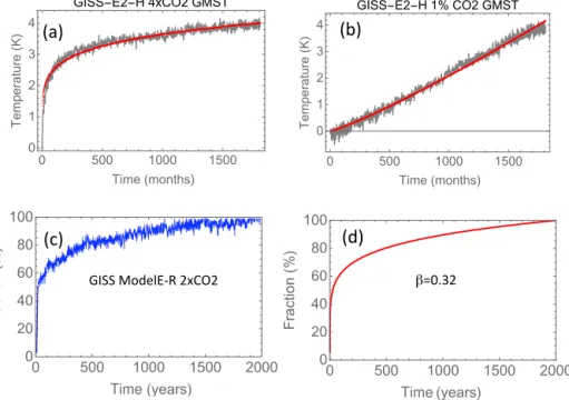
2 concentration, the latter corresponds to exponentially grow-ing concentration. Climate model runs with linearly growgrow-ing forcing are of course more realistic than step-function runs, but both have been conducted as part of the CMIP5 project. Examples are 150-year-long simulations of the GISS-E2-H model with a sudden quadrupling of the CO2concentration (Fig. C1a) and a 1 % per year increase in the CO2 concentra-tion (Fig. C1b). A fit of the LRM-scaling responseT ∼tβT/2

to the GISS-model result in Fig. C1a yieldsβT ≈0.32, and

the solution is shown as the red curve in the figure. The so-lution of the form T ∼tβT/2+1 _{is shown as the red curve}

in Fig. C1b. The fit to the tail of the step-function response looks good in the 150-year duration of the simulation, but the divergence of the solution ast→ ∞indicates that the power-law tail withβT >0 is unrealistic for sufficiently large times.

There exist few AOGCM simulations that investigate the re-sponse to such idealised forcing on a millennium timescale. In Hansen et al. (2011) some figures with results of such runs are given. Figure C1c is an adaptation of Fig. 3 in Hansen et al. (2011), which shows a 2000-year-long run of the GISS ModelE-R, and Fig. C1d shows a plot of the func-tionctβT/2+1_with_β₌₀_._{32. It demonstrates that at least this}

particular AOGCM exhibits the power-law tail in the temper-ature response on timescales of up to 2 millennia.

Note that the βT ≈0.32 obtained for the LRM model

on long timescales is smaller than theβT ≈ 0.75 estimated

from the spectra of the residual of the instrumental data after the response to the deterministic forcing has been subtracted (Rypdal and Rypdal, 2014). If we produce such residuals by subtracting the red curves from the GISS-model curves in Fig. C1a, b, the result looks like fractional Gaussian noise (fGn) with a spectral exponentβ ≈0.65. As mentioned in Sect. 2.1 an fGnxβ(t) characterised by the spectral exponent βis produced by the convolution integral Eq. (2) in the main paper if the response kernel isG(t)∼tβ/2−1and the forcing functionF(t) is white Gaussian noisex0(t) (white noise is an fGn withβ=0). In other words, we have

xβ(t)= ∞

Z

−∞

t′β/2−1H(t−t′)x0(t′) dt′, (C1)

whereH(t) is the unit step function. By using the convo-lution theorem for the Fourier transform, it is easily shown (Rypdal et al., 2015) that ifF(t) is an fGn with spectral ex-ponentβF and the response function has exponentβT, then

the convolution will produce an fGn withβ=βT +βF:

xβ(t)= ∞

Z

−∞

t′βT/2−1_H₍_t₋_t′₎_x βF(t

′_{) d}_t′_. _(C2)

In Rypdal et al. (2015) it was suggested that the discrepancy between the spectral exponentβof residuals in observed and simulated GMST records could be explained by assuming some long-range memory (βF >0) in the stochastic forcing.

(12)

GISS ModelE‐R 2xCO2 β=0.32

(c)

(d)

��

0 500 1000 1500

0 1 2 3 4

Time(months)

T

emperat

ure

(

K

)

GISS-E2-H 4xCO2 GMST

��

0 500 1000 1500

0 1 2 3 4

Time₍months₎

T

emperat

ure

(

K

)

GISS-E2-H 1%CO2 GMST

(a)

(b)

��

0 500 1000 1500 2000

0 20 40 60 80 100

Time(years)

F

ract

ion

(%)

��

0 500 1000 1500 2000

0 20 40 60 80 100

Time (years)

F

ract

ion

(%)

Figure C1.Panel(a): LRM response model fitc1tβT/2(red) to the GISS-E2-H model response to an abrupt quadrupling of atmospheric

CO₂(grey). The fit yieldsβT =0.32. Panel(b): the LRM-response model solutionc2tβT/2+1withβT =0.32 (red) and the GISS-E2-H

(13)

Appendix D: Two-box vs. LRM fitting to GCM results

Geoffroy et al. (2013) have considered 16 runs of different CMIP5 models with step-function forcing, and fitted the re-sponse in the two-box model to the CMIP5-model rere-sponses. There are four fitting parameters, and the fits are generally good. There is, however, a wide scatter in the fitting param-eters between the different models, which may be an indica-tion of overfitting. In Fig. D1 the surface temperature solu-tion to the two-box model,

T1(t)= [Str(1−exp(−t /τtr))

+(Seq−Str)(1−exp(−t /τeq))]F4×CO2, (D1)

and to the LRM model,

T₁(t)=ctβT/2_F

4×CO2, (D2)

have been fitted to simulation results for the GMST of cli-mate models with step-forcing, F(t)=F4×CO2H(t). Here

F4×CO2 ≈ 8.61 Wm

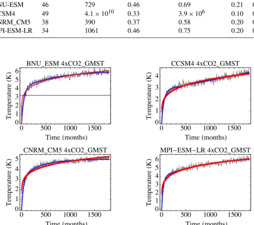
−2_{is the forcing associated with a} qua-drupling of the atmospheric CO2 concentration. The fitting parameters obtained are given in Table 1.

The LRM model in general gives a poorer fit on the short timescales. This is not surprising, since the LRM response

ctβT/2 _{has an infinite derivative at}_t₌₀_._{However, a much}

better approximation is obtained if we fit the LRM model only in the interval (0,100) months, but thenβT is raised to

approximately 0.75. If we implement a four-parameter model with one power law (βT ≈0.75) up to 100 months and

an-other (βT ≈0.35) fort >100 months, we obtain fits

com-parable to the two-exponential model. There is a wide scatter in the model parameters for the two-box model. Note partic-ularly the huge values forτeqandSeqfor the CCSM4 model. The long timescale tail is not captured by a reasonable expo-nential but is well approximated by a reasonable power law. On the other hand, the scatter in the LRM-model parameters is small. All this indicates that the two-box model may suffer from overfitting in some cases.

When projections are limited to 2200 CE, there is no prac-tical difference between using a power-law response kernel (the LRM model) and the exponential kernel (the two-box model). This is illustrated in Fig. D2, where we compute the response for the exponential CO2 concentration model withτC=33 years and the two-box model parameters cor-responding to the GISS-E2-H model and the CNRM_CM5 models. The parameters for the two models differ signifi-cantly, but the projections are almost identical. Moreover, they are very similar to the projections in Fig. 5a, where the temperature response is produced by the LRM model withτC=33 years and βT =0.35. This demonstrates that

(14)

Table D1.Parameters estimated by fitting Eqs. (D1) and (D2) to the climate model responses to an abrupt quadrupling of atmospheric CO2 shown in Fig. D1. The table shows the parameters obtained by the Mathematica routine FindFit.

Model τ₁(Months) τ₂(Months) Str(km2W−1) Seq(km2W−1) c βT

GISS-E2-H 26 663 0.29 0.46 0.14 0.32

BNU-ESM 46 729 0.46 0.69 0.21 0.33

CCSM4 49 4.1×1010 0.33 3.9×106 0.10 0.40

CNRM_CM5 38 390 0.37 0.58 0.20 0.31

MPI-ESM-LR 34 1061 0.46 0.75 0.20 0.33

0 500 1000 1500 0

1 2 3 4 5 6

TimeHmonthsL

Temper

atur

e

H

K

L

BNU_ESM 4xCO2_GMST

0 500 1000 1500 0

1 2 3 4

TimeHmonthsL

Temper

atur

e

H

K

L

CCSM4 4xCO2_GMST

0 500 1000 1500 0

1 2 3 4 5

TimeHmonthsL

Temper

atur

e

H

K

L

CNRM_CM5 4xCO2_GMST

0 500 1000 1500 0

1 2 3 4 5 6

TimeHmonthsL

Temper

atur

e

H

K

L

MPI-ESM-LR 4xCO2_GMST

Figure D1.Blue curves: fit of the two-exponential response to the climate model responses to an abrupt quadrupling of atmospheric CO2

concentration. Red curves: fit of the LRM-scaling response. The expressions fitted are found in the caption of Table 1 and the coefficients estimated are shown in this table.

��

1900 1950 2000 2050 2100 2150 2200 0

1 2 3 4

Year

Te

m

p

e

ra

tu

re

(

K

)

GMSTτC=33 yr,τtr=26 months,τeq=663 months

1900 1950 2000 2050 2100 2150 2200 0

1 2 3 4

Year

Te

m

p

e

ra

tu

re

(

K

)

GMSTτC=33 yr,τtr=38 months,τeq=390 months

(a)

(b)

Figure D2.The evolution of the GMST according to the two-box model for the CO2concentration scenarios shown in Fig. 4a and c. Panel

(15)

Appendix E: Divergences, causality and initial conditions

If G(t) is a power law, the integral over prehistory t∈

(−∞,0) may lead to paradoxes, such as divergences of the integral. The solution to the paradox is to interpret the power law as an approximation, for instance to a superposition of exponential response kernels. For a white-noise forcing this corresponds to an aggregation of Ornstein–Uhlenbeck (OU) processes, which are known to have the potential to produce a process that is a very good approximation to a fractional Gaussian noise (fGn) up to the timescale corresponding to the OU process with the greatest correlation time (Granger, 1980).

The scaling properties on scales of decades and longer arise from the heat transport within the oceans. This transport exhibits a maximum response time, which will provide an upper (exponential) cut-off of the power-law response func-tion, but the characteristic time of this cut-off may be cen-turies or millennia. Fraedrich and Blender (2003) state in their abstract: “Scaling up to decades is demonstrated in ob-servations and coupled atmosphere–ocean models with com-plex and mixed-layer oceans. Only with the comcom-plex ocean model the simulated power laws extend up to centuries.”

If we do not treat the power law as an approximation, we have to deal with the divergences of the integral

1T(t)= t

Z

−∞

G(t−t′)F(t′) dt′, (E1)

whereG(s)=sβT/2−1_{. If we consider the unit step-function}

forcingF(t)=H(t) andβT 6=0, the integral is

1T(t)= lim

ǫ→0+

t

Z

ǫ

(t−t′)βT/2−1_d_t′₌ _lim ǫ→0+

t

Z

ǫ

sβT/2−1_s

= lim

ǫ→0+

2

βT

tβT/2₋_ǫβT/2_. _(E2)

Clearly 1T(t) diverges as t→ ∞ if βT >0, but it also

diverges ifβT <0 (asǫ→0+). ForβT =0 there is a

loga-rithmic divergence in both limits.

For physically meaningful results theβT >0 case requires

some sort of cut-off (e.g. an exponential tail) for sufficiently larget, and theβT <0 case requires an elimination of the

strong singularity ofG(s) ats=0. As shown in Appendix D, AOGCMs in the CMIP5 ensemble with step-function forc-ing indicate a power-law response for large sat least up to 150 years (and the GISS-E2-R model up to 2000 years) with

βT ≈ 0.35, soβT >0 is the case of interest for the global

temperature response. The AOGCMs are also well approxi-mated by an exponential response in the limit s→0 (fors

up to a few years), so an exponential truncation in this high-frequency limit is also appropriate.

The truncation of the power-law kernels is a physical, and not a technical mathematical issue. It is an approximation to a hierarchy of exponential responses. With this interpretation the divergences evaporate. Below is a more detailed outline of this philosophy in an energy balance context. Let us take as a starting point the simple zero-dimensional EBM before linearisation of the Stefan–Boltzmann law:

CdT

dt = −ǫσST

4₊_I₍_t₎_, _(E3)

where T is surface temperature in Kelvin, C is an effec-tive heat capacity per area of the earth’s surface,σS is the

Stefan–Boltzmann constant, ǫ is an effective emissivity of the atmosphere, andI(t) is the incoming radiative flux den-sity at the top of the atmosphere. LetI0=I(0) be the ini-tial incoming flux,F(t)=I(t)−I0 is the radiative forcing,

Teq=(I0/ǫσS)1/4 is the equilibrium temperature at t=0, 1T(t)=T(t)−Teq is the temperature anomaly measured relative to the initial equilibrium temperature, and 1T0=

1T(0) is this anomaly att=0. Note thatF here is the per-turbation of the radiative flux with respect to the initial flux

I0and not with respect to the fluxǫσST₀4 that would be in

equilibrium with the initial temperature T0. The linearised EBM for the temperature change relative to the temperature

T_eq(the one-box model) is

d1T

dt = −ν1T+F(t), 1T(0)=1T0, (E4)

where ν=4ǫσSTeq3/C, F(t)=F(t)/C. By definition F(0)= [I(0)−I0]/C=0. This is Eq. (1) and Eq. (A1) with slightly different notation. The solution to the initial value problem (i.v.p.) Eq. (E4), with the initial condition

1T(0)=1T0, takes the form

1Ti.v.p.=

t

Z

0

G(t−t′)F(t′) dt′+1T0e−νt, (E5)

where G(s)=exp(−νs). The generalisation to a linear, causal response model, where G(s) is not necessarily ex-ponential, involves extending the integration domain in Eq. (E5) to the interval (−∞, t):

1Tr.m.(t)=

t

Z

−∞

G(t−t′)F(t′) dt′. (E6)

From the initial condition1T(0)r.m.=1T0Eq. (E6) yields

1T0= 0 Z

−∞

G(−t′)F₍t′) dt′. (E7)

(16)

the forcingF₍t) fort∈(t,0):

1T0= 0 Z

−∞

eνt′F(t′) dt′. (E8)

For the exponential response there is no “divergence issue” in Eq. (E6). Neither is there such an issue for the two-exponential solution to the two-box model (Geoffroy et al., 2013). An “N-box model” exhibits a response function for the temperature in each box which is a superposition of expo-nentials;G(s)=PN_i=₁aiexp(−νis). For the surface (mixed

layer) box the temperature anomaly takes the form

1Tr.m.(t)=

N

X

i=1

aie−νit t

Z

−∞

eνit′_F₍_t′_{) d}_t′_. _(E9)

On the other hand, the N-box initial value problem has a solution of the form

1Ti.v.p.(t)= N

X

i=1

aie−νit t

Z

0

eνit′_F₍_t′_{) d}_t′₊ N

X

i=1

bie−νit, (E10)

where the coefficientbi is linearly related to the initial

tem-peratures of each box: bi=PNj=1MijT0j. The condition

e

Ti.v.p.(t)=Ter.m.(t) now yields the relations between the ini-tial temperatures and the prehistory of the forcing:

N

X

j=1

Mij1T0j=ai

0 Z

−∞

eνit′_F₍_t′_{) d}_t′ _for _i₌₁_{, . . ., N.} _(E11)

With a white-noise forcingF(t), Eq. (E4) is the Itô stochas-tic differential equation (in physics often called the Langevin equation). The solution is the Ornstein–Uhlenbeck (OU) stochastic process, which in discrete time corresponds to the first-order autoregressive (AR(1)) process. The power spec-tral density of this process is essentially a Lorentzian func-tion, which means that the high-frequency (f ≫ν) part of the spectrum has the form∼f−2and the low-frequency part

∼f0. This means that if the climate response were well described by a one-box EBM we could use a power-law response model with βT ≈2 on timescales much shorter

than the correlation timeτc=ν−1. On these timescales the stochastic process exhibits the characteristics of a Brown-ian motion (Wiener process), which is a self-similar process with spectral indexβ=2. This process is non-stationary and hence suffers from the divergences that we are worried about. However, even though the Brownian motion diverges, the OU process does not because of the flattening of the spectrum for

f ≪ν.

Both observation data and AOGCMs indicate that the one-box EBM is inadequate, but the considerations above are equally valid for anN-box model, for which the white-noise forcing gives rise to an aggregation of OU processes with different νi. Such an aggregation is known to be able to

produce a process with an approximate power-law spectrum with 0< β <2 on timescalesτ < ν_min−1 (Granger, 1980).

Lovejoy et al. (2013) specifically argue that volcanic forc-ing may have a scalforc-ing exponentβF ≈ 0.4, and hence the

convergence criterionβ=βT +βf <1 then requires βT <

0.6. One remark on this is that the above discussion shows that theβ <1 criterion is not necessary on timescales shorter thanτ < ν_min−1. However, observation indicates thatβ <1, so this does not invalidate the argument of Lovejoy et al. (2013). More important is that in recent papers the response to vol-canic forcing has been subtracted from both instrumental and multiproxy reconstruction data (Rypdal and Rypdal, 2014) and from millennium-long AOGCM simulations (Østvand et al., 2014), and the residuals have been analysed forβwithout finding a detectable influence of the volcanic forcing onβ. The same is seen by comparing control runs of the AOGCMs with those driven by volcanic forcing (Østvand et al., 2014). The importance of including the prehistory of the energy-flux imbalance when deriving projections for future change can be illustrated by considering a prehistory consisting of volcanic forcingF_V(t) only. The particular feature of vol-canic forcing is that it consists of a succession of negative spikes in the radiation flux. If we assume that the timet=0 is in a period with no volcanic forcing, we can for illustra-tion think of the forcing as a succession of negative forcing events of short duration, randomly distributed in time with typically longer waiting times between events than durations. Let us further assume that the climate response is so slow that

G(t) varies by a small amount over the mean waiting time. Hence, there exist time intervals of duration1t which are short enough forG(t) to be nearly constant over the interval but long enough to have a sufficient number of large volcanic eruptions to estimate a mean volcanic forcingF_V. This as-sumption is not very good in practice, but let us use it for illustration. Under this assumption we can approximate the integral

t1+1t /_Z 2

t1−1t /2

G(t−t′)F_V(t′)dt′ ≈G(t−t1)

t1+1t /_Z 2

t1−1t /2

F_V(t′) dt

=G(t−t1)FV1t, (E12)

(17)

1TV(t)=FV t

Z

−∞

G(t−t1) dt1

=F_V ∞

Z

0

G(s) dsdef= −1Tvolc. (E13)

This result is meaningful only if the integralR₀∞G(s) ds is finite, i.e. if power-law response kernels are properly trun-cated. The obvious, but still interesting, observation is that volcanic forcing keeps the temperature, when averaged over the timescale 1t, on a constant levelTeq−1Tvolc, i.e. the time-averaged temperature is1Tvolc lower than the temper-ature at which the climate system is in equilibrium during times with no volcanic forcing.

Assume some additional (e.g. anthropogenic) forcing F_A(t), for whichF_A=0 for t≤0. Then the total temper-ature anomaly fort >0 would be

1T(t)=1TV(t)+1TA(t)

= −1T_volc+ t

Z

0

G(t−t′)F_A₍t′) dt′, (E14)

implying that the temperature starts changing in response to this forcing from a non-equilibrium initial state. However, the statistics of volcanic forcing is more challenging than as-sumed above, and one has to consider the possibility of long periods with zero forcing, longer than the largest tempera-ture relaxation time reflected in the response functionG(t). If such a quiet period starts at timetq, then the temperature

fort > tqis

1T(t)=F_V ∞

Z

t−tq

G(s) ds+ t

Z

0

G(t−t′)F_A(t′) dt′, (E15)

and since the integral over the tail of G(s) is assumed to be finite (there exists a maximum relaxation time constant

τmax), the first term on the right of Eq. (E15) will vanish if

t > tq+τmax. In other words, if the time of observation has been preceded by a very long period of weak volcanic forc-ing the additionally forced temperature change may be unaf-fected by the non-equilibrium imposed by volcanic forcing. If we consider, as another example, that “normal” volcanic forcing is resumed at t=0 after a pause of the length of

|tq|> τmax, then1T according to Eq. (E15) grows from zero towards the expression in Eq. (E14) ast grows beyondtmax. Hence, during the transient periodt∈(0, τmax) there may be a volcanic cooling that counteracts anthropogenic warming, provided there was a long pause in volcanic forcing preced-ing the era of anthropogenic forcpreced-ing.

The discussion made here serves to illustrate that the non-equilibrium of the radiative flux balance att=0 may influ-ence the subsequent temperature evolution and that volcanic forcing may be the source of such an imbalance. Knowl-edge about the history of volcanic forcing in the time interval (−τmax, t) can be helpful in assessing the influence of vol-canic forcing on the long-term temperature evolution in the Anthropocene. In the present paper the implicit assumption has been made that Eq. (E14) is valid, i.e. that there is no long pause in volcanic forcing in the period extending from 1880−τmaxto 2200 CE. Hence, this forcing only represents a constant downshift of the temperature. This assumption may deserve closer scrutiny.

Appendix F: Non-stationarity of the CO₂response

In Sect. 2.2 we found (by comparing Fig. 4b and c) that the LRM CO2response withβC=1.6 gives approximately the same evolution of CO2concentration up to 2200 CE as a re-sponse where 50 % of the emitted CO2 is absorbed by the surface almost immediately and the remainder decays expo-nentially with a time constantτC=300 years. This is analo-gous to the situation with the temperature response, where an LRM response gives very similar results to a two-exponential response with appropriate fitting of model parameters (see Appendix D). The most important difference is that theβC parameter is larger than unity. A step-function emission rate

R(t)=H(t) will give rise to a CO2concentration that grows like (2αT/βC)tβC/2. This non-stationarity (divergence) of the response ast→ ∞is reasonable, since the surface will not be able to absorb a sufficient fraction of the constantly emit-ted CO2to establish a new equilibrium. The exponential re-sponse kernel Eq. (6), on the other hand, yields the rere-sponse

r[1−exp(−t /τC)]to the step forcing. This implies the es-tablishment of a new equilibrium CO2 concentration after

t≫τC. This has little consequence as long as we consider projection only up to 2200 CE (andτC≈ 300 years). On a millennium timescale we have the positive ice-age feedback, by which warming may lead to net release of CO2 to the atmosphere, and hence lead to a continuing growth of CO2 concentration. It is assumed to be important in the trigger-ing of glacial–interglacial transitions, although it is not very well understood. On timescales of hundreds of kiloyears, we have the negative carbon-weathering-cycle feedback that will eventually lead to a carbon-cycle equilibrium. The most in-teresting feature of this feedback in the present context is that it suggests that the anthropogenic global warming event may last for such a long time in the absence of effective carbon sequestration measures (Archer, 2010).

(18)

that the variance increases with time as tβC−1_{, which is not}

(19)

The Supplement related to this article is available online at doi:10.5194/esd-7-51-2016-supplement.

Acknowledgements. This work was funded by project

no. 229754 under the Norwegian Research Council KLI-MAFORSK programme.

Edited by: R. Krishnan

References

Archer, D.: The Global Carbon Cycle, Princeton Primers in Cli-mate, Princeton University Press, Princeton, Chapter 12, 287– 295, 2010.

Allen, M. R., Frame, D. J., Huntingford, C., Jones, C. D., Lowe, J. A., Meinshausen, M., and Meinshausen, N.: Warming caused by cumulative carbon emissions towards the trillionth tonne, Nature, 458, 1163–1166, doi:10.1038/nature08019, 2009.

Anderegg, W. R. L., Prall, J. W, Harold, J., and Schneider, S. H.: Expert credibility in climate change, P. Natl. Acad. Sci., 107, 12107–12109, doi:10.1073/pnas.1003187107, 2010.

Bender, M. L.: Paleoclimate, Princeton Primers in Climate, Prince-ton University Press, PrincePrince-ton, Chapter 10, 235–263, 2013. Beran, J.: Statistics for Long-memory Processes, Monographs on

statistics and applied probability, Chapman& Hall/CRC, Boca Raton, 1994.

Brohan, P., Kennedy, J. J., Harris, I., Tett, S. F. B., and Jones, P. D.: Uncertainty estimates in regional and global observed tempera-ture changes: A new data set from 1850, J. Geophys. Res, 111, D12106, doi:10.1029/2005JD006548, 2006.

Budyko, M. I.: The effect of solar radiation variations on the climate of the Earth, Tellus, 21, 611–619, 1969.

Cook, J., Nuccitelli, D., Green, S. A., Richardson, M., Winkler, B., Painting, R., Way, R., Jacobs, P., and Skuce, A. : Quantifying the consensus on anthropogenic global warming in the scien-tific literature, Environ. Res. Lett. 8, 024024, doi:10.1088/1748-9326/8/2/024024, 2013.

den Elzen, M., Meinshausen, M., and van Vuuren, D.: Multi-gas emission envelopes to meet greenhouse Multi-gas concen-tration targets: costs versus certainty of limiting tem-perature increase, Global Environ. Change, 17, 260–280, doi:10.1016/j.gloenvcha.2006.10.003, 2007.

Geoffroy, O., Saint-Martin, D., Olivié, D. J. L., Voldoire, A., Bellon, G., and Tytcá, S.: Transient Climate Response in a Two-Layer Energy-Balance Model. Part I: Analytical Solution and Parame-ter Calibration Using CMIP5 AOGCM Experiments, J. Climate, 6, 1841–1857, doi:10.1175/JCLI-D-12-00195.1, 2013.

Fraedrich, K. and Blender, R.: Scaling of Atmosphere and Ocean Temperature Correlations in Observations and Climate Models, Phys. Rev. Lett., 90, 108501–10854, doi:10.1103/PhysRevLett.90.108501, 2003.

Granger, C. W. J.: Long Memory Relationships and the aggregation of dynamical models, J. Econometrics, 14, 227–238, 1980. Hansen, J., Sato, M., Kharecha, P., and von Schuckmann, K.:

Earth’s energy imbalance and implications, Atmos. Chem. Phys., 11, 13421–13449, doi:10.5194/acp-11-13421-2011, 2011.

Lenton, T. M., Held, H., Kriegler, E., Hall J. W., Lucht, W., Rahmstorf, S., and Schellnhuber, H. J.: Tipping elements in the Earth’s climate system, P. Natl. Acad. Sci., 105, 1786–1793, doi:10.1073/pnas.0705414105, 2008.

Lovejoy, C., Schehrtzer, D., and Varon, D.: Do GCMs predict climate. . . or macroweather?, Earth Syst. Dynam., 4, 439–454, doi:10.5194/esd-4-439-2013, 2013.

Stocker, T. F., Qin, D., Plattner, G.-K., Tignor, M., Allen, S. K., Boschung, J., Nauels, A., Xia, Y., Bex, V., and Midgley, P. M. (Eds.).: IPCC, 2013: Climate Change 2013: The Physical Sci-ence Basis. Contribution of Working Group I to the Fifth Assess-ment Report of the IntergovernAssess-mental Panel on Climate Change, Cambridge University Press, Cambridge, UK and New York, NY, USA, 1535 pp., 2013.

Joos, F., Roth, R., Fuglestvedt, J. S., Peters, G. P., Enting, I. G., von Bloh, W., Brovkin, V., Burke, E. J., Eby, M., Edwards, N. R., Friedrich, T., Frölicher, T. L., Halloran, P. R., Holden, P. B., Jones, C., Kleinen, T., Mackenzie, F. T., Matsumoto, K., Meinshausen, M., Plattner, G.-K., Reisinger, A., Segschneider, J., Shaffer, G., Steinacher, M., Strassmann, K., Tanaka, K., Tmermann, A., and Weaver, A. J.: Carbon dioxide and climate im-pulse response functions for the computation of greenhouse gas metrics: a multi-model analysis, Atmos. Chem. Phys., 13, 2793– 2825, doi:10.5194/acp-13-2793-2013, 2013.

Le Quéré, C., Moriarty, R., Andrew, R. M., Peters, G. P., Ciais, P., Friedlingstein, P., Jones, S. D., Sitch, S., Tans, P., Arneth, A., Boden, T. A., Bopp, L., Bozec, Y., Canadell, J. G., Cheval-lier, F., Cosca, C. E., Harris, I., Hoppema, M., Houghton, R. A., House, J. I., Jain, A., Johannessen, T., Kato, E., Keeling, R. F., Kitidis, V., Klein Goldewijk, K., Koven, C., Landa, C. S., Land-schützer, P., Lenton, A., Lima, I. D., Marland, G., Mathis, J. T., Metzl, N., Nojiri, Y., Olsen, A., Ono, T., Peters, W., Pfeil, B., Poulter, B., Raupach, M. R., Regnier, P., Rödenbeck, C., Saito, S., Salisbury, J. E., Schuster, U., Schwinger, J., Séférian, R., Segschneider, J., Steinhoff, T., Stocker, B. D., Sutton, A. J., Taka-hashi, T., Tilbrook, B., van der Werf, G. R., Viovy, N., Wang, Y.-P., Wanninkhof, R., Wiltshire, A., and Zeng, N.: Global car-bon budget 2014, Earth Syst. Sci. Data Discuss., 7, 521–610, doi:10.5194/essdd-7-521-2014, 2014.

Matthews, H. D., Gillett, M. P., Stott, P. A., and Zickfeld, K.: The proportionality of global warming to cumulative carbon emis-sions, Nature, 459, 1129–132, doi:10.1038/nature08047, 2009. Meehl, G. A., Washington,W. M., Amman,C. M., Arblaster, J. M.,

Wigley, T. M., and Tebaldi, C.: Combinations of Natural and An-thropogenic Forcings in Twentieth-Century Climate, J. Climate, 17, 3721–3727, 2004.

Meinshausen, M., Smith, S. J., Calvin, K., Daniel, J. S., Kainuma, M. L. T., Lamarque, J.-F., Matsumoto, K., Montzka, S. A., Raper, S. C. B., Riahi, K., Thomson, A., Velders, G. J. M., van Vu-uren, D. P. P.: The RCP greenhouse gas concentrations and their extensions from 1765 to 2300, Clim. Change, 11, 2013–241, doi:10.1007/s10584-011-0156-z, 2011.

Myhre, G., Highwood, J., Shine, K. P., and Stordahl, F.: New esti-mates of radiative forcing due to well-mixed greenhouse gases, Geophys. Res. Lett., 25, 2715–2718, 1998.

(20)

Rypdal, K.: Global temperature response to radiative forcing: Solar cycle versus volcanic eruptions, J. Geophys. Res., 117, D06115, doi:10.1029/2011JD017283, 2012.

Rypdal, M. and Rypdal, K.: Long-memory effects in linear-response models of Earth’s temperature and implications for future global warming, J. Climate, 27, 5240–5258, doi:10.1175/JCLI-D-13-00296.1, 2014.

Rypdal, K., Rypdal, M., and H.-B. Fredriksen: Spatiotemporal Long-Range Persistence in Earth’s Temperature Field: Analysis of Stochastic-Diffusive Energy Balance Models, J. Climate, 28, 8379–8395, doi:10.1175/JCLI-D-15-0183.1, 2015.

Schwartz, S. E.: Heat capacity, time constant, and sensitivity of the Earth’s climate system, J. Geophys. Res., 112, D24S05, doi:10.1029/2007JD008746, 2007.

Sellers, W. D.: A global climate model based on the energy balance of the Earth-atmosphere system, J. Appl. Meteorol., 8, 392–400, 1969.

Solomon, L.: The Deniers. The world-renowned scientists who stood up against global warming hysteria, political persecution and fraud, Richard Viglante Books, 1–239. 2008.

Stocker, T.: The Closing Door of Climate Targets, Science, 339, 280–282, doi:10.1126/science.1232468, 2013.