A global coupled Eulerian-Lagrangian model and 1 × 1 km CO<sub>2</sub> surface flux dataset for high-resolution atmospheric CO<sub>2</sub> transport simulations

(1)

GMDD

4, 2047–2080, 2011

A global coupled Eulerian-Lagrangian

model

A. Ganshin et al.

Title Page

Abstract Introduction

Conclusions References

Tables Figures

◭ ◮

Back Close

Full Screen / Esc

Printer-friendly Version Interactive Discussion

Discussion

P

a

per

|

Dis

cussion

P

a

per

|

Discussion

P

a

per

|

Discussio

n

P

a

per

|

Geosci. Model Dev. Discuss., 4, 2047–2080, 2011 www.geosci-model-dev-discuss.net/4/2047/2011/ doi:10.5194/gmdd-4-2047-2011

Geoscientific Model Development Discussions

This discussion paper is/has been under review for the journal Geoscientific Model Development (GMD). Please refer to the corresponding final paper in GMD if available.

A global coupled Eulerian-Lagrangian

model and 1

×

1 km CO

₂

surface flux

dataset for high-resolution atmospheric

CO

₂

transport simulations

A. Ganshin1, T. Oda2,*, M. Saito2,**, S. Maksyutov2, V. Valsala2, R. J. Andres3, R. Fischer4, D. Lowry4, A. Lukyanov1, H. Matsueda5, E. G. Nisbet4, M. Rigby6, Y. Sawa5, R. Toumi7, K. Tsuboi5, A. Varlagin8, and R. Zhuravlev1

1

Central Aerological Observatory, Dolgoprudny, Russia

2

Center for Global Environmental Research, National Institute for Environmental Studies, Tsukuba, Japan

3

Carbon Dioxide Information Analysis Center, Oak Ridge National Laboratory, Oak Ridge, USA

4

Department of Geology, Royal Holloway, University of London, London, UK

5

Meteorological Research Institute, Tsukuba, Japan

6

Center for Global Change Science, Massachusetts Institute of Technology, Cambridge, MA, USA

7

(2)

GMDD

4, 2047–2080, 2011

model

A. Ganshin et al.

Title Page

Tables Figures

◭ ◮

Back Close

Full Screen / Esc

Discussion

P

a

per

|

Dis

cussion

P

a

per

|

Discussion

P

a

per

|

Discussio

n

P

a

per

|

8

A.N. Severtsov Institute of Ecology and Evolution, Russia

∗_{now at: Cooperative Institute for Research in the Atmosphere, Colorado State University,}

Fort Collins, USA/Earth System Research Laboratory, National Oceanic and Atmosphere Administration, Boulder, USA

∗∗_{now at: LSCE, Gif Sur Yvette, France}

Received: 26 July 2011 – Accepted: 21 August 2011 – Published: 24 August 2011

Correspondence to: A. Ganshin (alexander.ganshin@gmail.com)

(3)

GMDD

4, 2047–2080, 2011

model

A. Ganshin et al.

Title Page

Tables Figures

◭ ◮

Back Close

Full Screen / Esc

Discussion

P

a

per

|

Dis

cussion

P

a

per

|

Discussion

P

a

per

|

Discussio

n

P

a

per

|

Abstract

We designed a method to simulate atmospheric CO2 concentrations at several

con-tinuous observation sites around the globe using surface fluxes at a very high spatial resolution. The simulations presented in this study were performed using a Lagrangian particle dispersion model coupled to a global atmospheric tracer transport model with

5

prescribed global surface CO2 flux maps at a 1×1 km resolution. The surface fluxes

used in the simulations were prepared by assembling the individual components of terrestrial, oceanic and fossil fuel CO2 fluxes. This experimental setup (i.e., a

trans-port model running at a medium resolution, coupled to a high-resolution Lagrangian particle dispersion model together with global surface fluxes at a very high

resolu-10

tion), which was designed to represent high-frequency variations in atmospheric CO₂ concentration, has not been reported at a global scale previously. Two sensitivity ex-periments were performed: (a) using the global transport model without coupling to the Lagrangian dispersion model, and (b) using the coupled model with a reduced res-olution of surface fluxes, in order to evaluate the performance of Eulerian-Lagrangian

15

coupling and the role of high-resolution fluxes in simulating high-frequency variations in atmospheric CO₂ concentrations. A correlation analysis between observed and simu-lated atmospheric CO2concentrations at selected locations revealed that the inclusion

of both Eulerian-Lagrangian coupling and resolution fluxes improves the high-frequency simulations of the model. The results highlight the potential of a coupled

20

Eulerian-Lagrangian model in simulating high-frequency atmospheric CO2

concentra-tions at many locaconcentra-tions worldwide. The model performs well in representing obser-vations of atmospheric CO₂ concentrations at high spatial and temporal resolutions, especially for coastal sites and sites located close to sources of large anthropogenic emissions. While this study focused on simulations of CO2concentrations, the model

25

(4)

GMDD

4, 2047–2080, 2011

model

A. Ganshin et al.

Title Page

Tables Figures

◭ ◮

Back Close

Full Screen / Esc

Discussion

P

a

per

|

Dis

cussion

P

a

per

|

Discussion

P

a

per

|

Discussio

n

P

a

per

|

1 Introduction

The anthropogenic emissions of greenhouse gases could potentially change the global average temperature, leading to global warming. The latest assessment report of the Intergovernmental Panel on Climate Change (IPCC-AR4) states that climate models are capable of reproducing the temperature trends observed in recent decades if they

5

are forced with increasing concentrations of anthropogenic greenhouse gas (IPCC, 2007). A major contributor to anthropogenic greenhouse gases in the atmosphere is carbon dioxide (CO2), which plays a key role in the global climate. Consequently,

esti-mations of CO2emissions are important in assessing its influence on ongoing climate

change. To understand the nature of CO₂cycling between the land, atmosphere and

10

ocean, it is necessary to calculate precisely the natural and anthropogenic fluxes of CO2and the temporal and spatial variability of CO2concentrations in the atmosphere.

Variations in CO₂ concentrations in the atmosphere are generally assessed using transport models with prescribed surface fluxes. Such modelling efforts are essential in order to inversely estimate the CO2fluxes between the atmosphere and land-ocean

15

surfaces using model-predicted quantities of atmospheric CO₂and corresponding ob-servations (Gurney et al., 2002). The essential elements required for modelling of atmospheric CO2 concentrations are a transport model, meteorological drivers, and

surface fluxes. Consequently, the accuracy of simulated concentrations is strongly de-pendent on the ability of the transport model to represent the observed variability of

20

atmospheric CO2 concentrations, thereby resulting in large differences in the outputs

of various models (Patra et al., 2008). Therefore, the faithful representation of CO₂ concentrations in transport models is an area of active research (Patra et al., 2008). In this study, we present a novel strategy to improve the performance of a transport model by coupling two essential components of modelling, as described below.

25

(5)

GMDD

4, 2047–2080, 2011

model

A. Ganshin et al.

Title Page

Tables Figures

◭ ◮

Back Close

Full Screen / Esc

Discussion

P

a

per

|

Dis

cussion

P

a

per

|

Discussion

P

a

per

|

Discussio

n

P

a

per

|

following a predetermined atmospheric velocity. One example of a Lagrangian model is a trajectory model in which the locations of air masses are traced using an imagi-nary particle. Lagrangian particle dispersion models (LPDM) are typical examples of extended trajectory models that utilize multiple particles to represent turbulence, dif-fusion and convection processes, in addition to the velocities of participles along

tra-5

jectory paths (e.g., Thomson, 1987). LPDMs can be run forward or backward in time. Forward simulations are generally employed to calculate the transport and dispersion of tracers from point sources, whereas backward simulations are used to estimate the potential contributions of pollutants from many sites to a single location. In this case, it is only necessary to perform one backward simulation from the receptor point, tracing

10

the given number of particles back to the possible source locations. Many previous studies have employed backward trajectory analyses of atmospheric tracer transport (Seibert et al., 1994; Stohl, 1996) and have utilized Lagrangian particle dispersion models (Lin et al., 2003; Seibert et al., 2004; Stohl et al., 2005; Folini et al., 2008; Lin et al., 2011).

15

In the case of Eulerian models, the evolution of the concentration field is described by partial di_fferential equations and is solved numerically using finite di_fference approx-imations (Richtmyer and Morton, 1967). Such models are applied to global-scale sim-ulations of the concentrations of atmospheric constituents and to the inverse modelling of surface fluxes (Gurney et al., 2002, 2004).

20

Each modelling approach has its advantages and disadvantages. For example, Eu-lerian models reproduce the seasonal cycle of atmospheric CO2 concentrations

rea-sonably well, but they su_ffer strongly from numerical di_ffusion, meaning that they per-form poorly in representing synoptic, super-synoptic and hourly variations. Lagrangian models, in contrast, do not suffer from numerical diffusion and they perform reasonably

25

(6)

GMDD

4, 2047–2080, 2011

model

A. Ganshin et al.

Title Page

Tables Figures

◭ ◮

Back Close

Full Screen / Esc

Discussion

P

a

per

|

Dis

cussion

P

a

per

|

Discussion

P

a

per

|

Discussio

n

P

a

per

|

Given the above limitations, it is reasonable to consider a hybrid model in which a Eulerian model is run to generate the global background concentrations of atmospheric constituents, which are then used as initial conditions for a Lagrangian model (e.g., Koyama et al., 2011). In the present study, we extended the approach introduced by Koyama et al. (2011) to a high-spatial-resolution case for simulating the concentrations

5

of atmospheric CO2in the same coupled Eulerian-Lagrangian modelling framework as

that used in the earlier study.

Several studies have reported the advantages of using coupled Eulerian-Lagrangian models, and some have used the WRF–STILT modelling system (Nehrkorn et al., 2010) to estimate the CO₂surface fluxes over North America (Gourdji et al., 2010). Rigby et

10

al. (2011) outlined a method for combining information on the emissions-mole fraction sensitivity from Eulerian and Lagrangian chemical transport models, for use in estimat-ing emissions. Previous studies have also suggested the use of high-resolution cou-pled Eulerian-Lagrangian models, especially for regional-scale studies. For instance, Trusilova et al. (2010) presented a coupled TM3-STILT model simulations based on the

15

nested atmospheric inversion scheme developed by Rodenbeck et al. (2009).

In the present study, we coupled a Eulerian model (National Institute for Environ-mental Studies-Transport Model, herein NIES-TM; Maksyutov et al., 2008, Belikov et al., 2011) and a Lagrangian particle dispersion model (FLEXPART; Stohl et al., 2005). We did not adopt the spatial coupling employed by similar models described above;

20

instead, we implemented a coupling at temporal boundaries. The coupled model is described in detail in Sect. 2.

A goal of this study is to demonstrate the merit of using a coupled model together with a newly developed high-resolution (1×1 km) global CO2flux dataset in simulating

high-frequency variations of observed atmospheric CO2 concentrations. The use of

25

(7)

GMDD

4, 2047–2080, 2011

model

A. Ganshin et al.

Title Page

Tables Figures

◭ ◮

Back Close

Full Screen / Esc

Discussion

P

a

per

|

Dis

cussion

P

a

per

|

Discussion

P

a

per

|

Discussio

n

P

a

per

|

A spatial radius of correlation on the order of 100 km or more is a commonly observed feature of wind and temperature fields (Buell, 1960, 1972; Gandin, 1965).

The remainder of this paper is organised as follows. The model, data and methods are described in Sect. 2, and CO2 emissions data and observations are presented

in Sect. 3. The model results and a discussion are presented in Sect. 4, and the

5

conclusions are provided in Sect. 5.

2 Model and methods

2.1 Lagrangian-Eulerian coupled model

Here, we describe the principles of the proposed Lagrangian-Eulerian coupled model. The concentration simulated by the Lagrangian model at the receptor (observation

10

location) is usually calculated as the integral of the residence time of all particles at each grid cell multiplied by the flux corresponding to that grid (Lin et al., 2003; Seibert et al., 2004). The concentration of CO₂in the Lagrangian model at any receptor point (corresponding to an observation site) can be written as follows (Holzer et al., 2000; Lin et al., 2003):

15

C(xr,tr)=

t_r

∫

t0

d t∫

V

d V I xr,tr|x,t

S(x,t)+∫

V

d V I xr,tr|x,t0

C(x,t0) (1)

where: C(xr,tr) – concentration at receptor pointxrat timetr;C(x,t0) – initial

concen-tration field at timet0, which is obtained from the background fields simulated by the

Eulerian model;I xr,tr|x,t

– influence function or Green’s function linking sources and sinksS(x,t) to the concentrations; andd V – volume element. The first term of Eq. (1)

20

denotes the concentration change at the receptor from sources/sinks in domainV dur-ing the time interval between initialization and observation. The second term refers to the contribution to the concentration at the receptor point by the advection of CO2from

(8)

GMDD

4, 2047–2080, 2011

model

A. Ganshin et al.

Title Page Abstract Introduction Conclusions References Tables Figures ◭ ◮ ◭ ◮ Back Close

Full Screen / Esc

Printer-friendly Version Interactive Discussion Discussion P a per | Dis cussion P a per | Discussion P a per | Discussio n P a per |

Lagrangian viewpoint, the influence function corresponds to the transition probability p xr,tr|x,t

along the air mass trajectories xn(t), calculated by the Lagrangian model

as follows:

p xr,tr|x,t

= 1

N

X

n=1

δ(xn(t)−x) (2)

where: N – number of air parcels emitted in the backward direction from the

recep-5

tor point, andδ – delta function representing the presence or absence of parcel i at locationx. Hence, in discrete form, Eq. (1) can be written as follows:

C(xr,tr)=

1 N T L IJK X i jk L X

l=o

S_{i jk}l

N

X

n=1

f_{i jk}l n+1

N

IJK

X

i jk

C_{i jk}B

N

X

n=1

f_{i jk}n (3)

where: i ,j,k – indices of a grid cell; l – time index; C_{i jk}B – initial background concen-tration from the Eulerian model;f_{i jk}n – 1 (parcel inside thei ,j,k cell), 0 (parcel outside

10

thei ,j,k cell);T – duration of trajectories; andL– number of steps when sources are

sampled by trajectories.

In the case of sampling surface sourcesF(x,y,t), we can consider their significance to a heighth(e.g., 500 m, which is the typical height of the planetary boundary layer):

S(x,t)=

( _F(x,y,t)mair

hρ(x,y,t)m_CO2,z≤h

0,z > h (4)

15

where: mair andmCO₂ – molar masses of air and CO2, respectively; and ¯ρ – average

air density belowh. Finally, we obtain

C(xr,tr)=

T mair

hNLρmCO₂

IJ

X

i j L

X

l=o

F_{i j}l

N

X

n=1

f_{i j}l n+1

N

IJK

X

i jk

C_{i jk}B

N

X

n=1

(9)

GMDD

4, 2047–2080, 2011

model

A. Ganshin et al.

Title Page

Tables Figures

◭ ◮

Back Close

Full Screen / Esc

Discussion

P

a

per

|

Dis

cussion

P

a

per

|

Discussion

P

a

per

|

Discussio

n

P

a

per

|

where the left term is associated with concentrations obtained from the Lagrangian model and the right term is the background CO₂concentration from the global Eulerian transport model.

In our coupled model, we use FLEXPART (run in backward mode) as the Lagrangian particle dispersion model and NIES-TM as the Eulerian global transport model (see the

5

Introduction for details). The background CO2 values on the model grid are obtained

by NIES-TM. We use a 2-day length of backward transport in FLEXPART. Gloor et al. (2001) found that a period on the order of 1.5 days is the timescale over it is still possible to discern, in the mixing ratio variations, the imprint of surface fluxes on the air parcel before its arrival at an observation point. In the present case, the background

10

CO₂values on the model grid points were provided by NIES-TM sampled 2 days prior to the observations.

2.2 Meteorological drivers

We used FLEXPART version 8.0 adapted to using JCDAS data (Onogi et al., 2007), which are provided on model levels and a Gaussian grid (40 model levels, T106 grid).

15

Because the original model was designed for use on a regular latitude-longitude hor-izontal grid (1.25◦×1.25◦) and on a hybrid sigma-pressure vertical grid on 40 levels, the required parameter values were obtained via bilinear horizontal interpolation at the model levels. The temporal resolution of input data is 6 hours. The numerical con-straints of the model (i.e., the maximum time-step required for a smooth tracking of

20

contributions of grid cell fluxes to the model concentrations) demand that the model time step (τ) is belowh/U, where his the size of the flux grid cells andU is the wind speed. At a wind speed ofU=50 km h−1, we obtainτ=2, 0.2, and 0.02 h for h=100, 10, and 1 km, respectively. Therefore, we used a period of 1 min as both the particle-transport time step and the flux-integration time step (i.e.,T/L of Eq. 5) for the 1-km

25

flux setup.

(10)

GMDD

4, 2047–2080, 2011

model

A. Ganshin et al.

Title Page

Tables Figures

◭ ◮

Back Close

Full Screen / Esc

Discussion

P

a

per

|

Dis

cussion

P

a

per

|

Discussion

P

a

per

|

Discussio

n

P

a

per

|

of 6 h. In this version of NIES-TM, the advection terms are solved by a second-order moment scheme (Prather, 1986). The implementation is documented by Belikov et al. (2011). The spatial resolution of the simulated NIES-TM background concentra-tion, as supplied for the FLEXPART model, was 2.5◦×2.5◦ on 15 sigma-levels; the corresponding temporal resolution was 1 h.

5

3 CO2fluxes and observations of atmospheric CO2concentrations

Three types of flux scenarios are commonly used in atmospheric CO₂ simulations: fossil fuel emissions, and biospheric and oceanic sources and sinks. These three fluxes collectively represent the major types of CO2 sources and sinks. Forest fires

should also be included as a component of biospheric flux. In the present simulations,

10

however, we excluded the contribution from forest fires assuming that it is reasonably small at the present observational sites, especially for the period of analysis used in this study. The above three fluxes are typically available at a spatial resolution of 1◦×1◦; however, this may be insufficient to represent strong, local emissions of CO2.

In previous coupled modelling studies (e.g., Koyama et al., 2011), the surface CO2

15

fluxes at 1◦×1◦ resolution were used for simulations of global atmospheric CO₂ con-centrations. However, as mentioned above, a flux dataset prepared at a high spatio-temporal resolution is sufficient for regional high-resolution simulations (Trusilova et al., 2010). In this study, we used 1◦×1◦ fluxes for global-scale Eulerian calculations of atmospheric CO2concentrations, and used 1×1 km fluxes for the Lagrangian model.

20

These contributions are combined in the coupled model, as described in the previous section. The 1◦×1◦ fluxes used for Eulerian simulations are the same as 1-km fluxes, with the only di_fference being resolution; the one exception is biospheric fluxes, for which we used those prepared by Nakatsuka and Maksyutov (2009) using an opti-mized CASA model.

(11)

GMDD

4, 2047–2080, 2011

model

A. Ganshin et al.

Title Page

Tables Figures

◭ ◮

Back Close

Full Screen / Esc

Discussion

P

a

per

|

Dis

cussion

P

a

per

|

Discussion

P

a

per

|

Discussio

n

P

a

per

|

3.1 Technique for handling fluxes on a 1×1 km grid

Here, we describe technical aspects of surface flux simulations at a very high resolu-tion. Because each of the global 1×1 km flux fields (e.g., biosphere, fossil and ocean fluxes) requires∼3.5 gigabytes (GB) of computer memory, it is inconvenient to operate with multiple layers of data at this resolution. To reduce the memory and disk storage

5

requirements, we propose the novel approach outlined below.

a. The 1×1 km surface flux fields at a given point are calculated in the model using a combination of data fields at high and medium resolutions. In the case of fossil fuel emissions, we multiply 1-km-resolution annual mean fluxes by a medium-resolution (1◦×1◦) spatially varying factor that represents the seasonal cycle at

10

a monthly time scale. This factor is derived from seasonally varying fossil-fuel-emissions data (Andres et al., 2011) at a resolution of 1◦×1◦, normalized to the annual mean. We use a land-cover mask at 1-km resolution to spatially redis-tribute the biospheric fluxes given at medium resolution and simulated separately for each of the 15 vegetation types. In this way, the memory usage and

computa-15

tional time are reduced considerably. A description of each dataset is given in the following subsections, and a summary of the combinations of fluxes used in the simulations is given in Table 1. The flux data at each model time step are obtained by linearly interpolating between the monthly fields, except for biospheric fluxes, which are provided a daily time step.

20

b. Even with the flux treatment outlined above, the memory requirements remained high. Consequently, we used sparse matrix storage (a method of representing matrices populated primarily with zeros; Tewarson, 1973) to reduce the memory demand for storing the anthropogenic emission field at 1-km resolution, because only ∼1 % of the elements in the matrix for anthropogenic emissions have

non-25

(12)

GMDD

4, 2047–2080, 2011

model

A. Ganshin et al.

Title Page

Tables Figures

◭ ◮

Back Close

Full Screen / Esc

Discussion

P

a

per

|

Dis

cussion

P

a

per

|

Discussion

P

a

per

|

Discussio

n

P

a

per

|

It is possible to use the same approach for land fluxes; however, this has little effect on storage requirements because only about 30 % of the elements have non-zero val-ues in this case. The combined application of the above two techniqval-ues (i.e., those described in a and b) reduces the memory demand to below 1.5 GB.

3.2 Fossil fuel CO2emissions 5

We used the Open source Data Inventory of Anthropogenic CO2emission (ODIAC)

in-ventory as fossil fuel CO2 emission fields, which is a global 1×1 km fossil fuel CO2

emission inventory based on country-level fuel consumption, a global power plant database and satellite observations of nightlight (Oda and Maksyutov, 2011). National annual total CO2 emissions were estimated using BP’s fuel consumption statistics for

10

coal, oil and natural gas (BP, 2008). The spatial distribution of point emissions was determined using power plant locations included in the CARbon Monitoring and Ac-tion (CARMA) power plant database (available at http://www.carma.org), and nightlight distributions were used for emissions from sources other than power plants. For fur-ther details of the ODIAC inventory, see Oda and Maksyutov (2011). We used US

15

Department of Energy Carbon Dioxide Information Analysis Center (CDIAC) monthly emission inventory (1◦×1◦ resolution) to create monthly fields (Andres et al., 2011). The CDIAC monthly emission inventory was created using the monthly fuel consump-tions of the top 21 emitting countries. For other countries, we used a proxy based on the data for the country among the top 21 with the most similar climate and economics.

20

Further details of this approach are given in Andres et al. (2011). In the present study, the CDIAC monthly inventory was used to distribute ODIAC annual totals into the 12 months of the year. Monthly values on 1◦×1◦grids were divided by annual totals at the grids, yielding 1◦×1◦normalized coefficient fields that were applied to 1×1 km ODIAC annual fields to derive monthly varying fields. For the Eulerian model simulation, we

25

(13)

GMDD

4, 2047–2080, 2011

model

A. Ganshin et al.

Title Page

Tables Figures

◭ ◮

Back Close

Full Screen / Esc

Discussion

P

a

per

|

Dis

cussion

P

a

per

|

Discussion

P

a

per

|

Discussio

n

P

a

per

|

3.3 Terrestrial biosphere fluxes

Vegetation CO2 fluxes were simulated with the terrestrial biospheric model VISIT (Ito

et al., 2007) at a resolution of 0.5◦×0.5◦and a daily time step for each of 15 vegetation types for each grid, closely following the procedure described by Saito et al. (2011), who simulated the ecosystem processes for four dominant vegetation types using

5

medium-resolution fluxes. However, for high-resolution fluxes the number of vegeta-tion types at each grid point (on a 0.5◦×0.5◦ grid) should be extended to include all possible types. The fluxes were interpolated spatially to each pixel of the vegetation map. Vegetation cover was derived from the Moderate Resolution Imaging Spectrora-diometer (MODIS) Land Cover Product (Friedl et al., 2002). The present study used a

10

global dataset in the Plate Carree projection (IGBP vegetation classification) at 30 arc-seconds (∼1 km). This product was derived from MODIS data for the year 2001 and is based on the reprojected mosaic exports from the MODIS MOD12Q1 v.004 dataset (available at http://duckwater.bu.edu/lc/datasets.html).

MODIS-IGBP classification divides terrestrial land covers into 17 biome types and

15

water body, whereas VISIT treats 15 biomes; consequently, the land cover classifica-tion was reconstituted to match that of VISIT algorithms (Saito et al., 2011).

3.4 Oceanic CO₂fluxes

Oceanic fluxes were obtained from a 4D-var assimilation system based on Valsala and Maksyutov (2010). In this system, an offline biogeochemical model was driven by

re-20

analysis ocean currents and was used to simulate the surface ocean partial pressure of CO2 (pCO2) and air-sea CO2 fluxes. The surface ocean pCO2 in the model was

constrained by ship-based observations of correspondingpCO₂ values and by clima-tological mean maps ofpCO2. The model employs a variational assimilation method

to constrain the simulated surface ocean pCO2 with reference to observations.

Cli-25

(14)

GMDD

4, 2047–2080, 2011

model

A. Ganshin et al.

Title Page

Tables Figures

◭ ◮

Back Close

Full Screen / Esc

Discussion

P

a

per

|

Dis

cussion

P

a

per

|

Discussion

P

a

per

|

Discussio

n

P

a

per

|

data were remapped onto a regular 1◦×1◦grid. This dataset was extended to coastal areas using land–ocean mask data (∼1-km resolution) derived from the MODIS global vegetation map described above.

3.5 Atmospheric CO2data

The model results were evaluated by comparison with atmospheric CO₂data obtained

5

at the following continuous observation sites, representative of both polluted and back-ground environments:

1. Fyodorovskoye tower, Russia;

2. Meteorological Research Institute (MRI) tower, Tsukuba, Japan;

3. Queen’s Tower, Imperial College London, London, UK;

10

4. Royall Holloway University, Egham, London, UK.

The Fyodorovskoye site is located in the central part of western Russia, near Tver (56◦27′N, 32◦55′E), within the Central Forest State Biosphere Natural Reserve (Mi-lyukova et al., 2002; Kurbatova et al., 2008). The reserve is located far from industrial or residential areas and is therefore largely free of air pollution. The measurement

15

tower is 29 m high and is located on a flat surface surrounded by homogenous vegeta-tion (spruce forest). The ambient CO2concentrations at heights of 0.20, 1.0, 2.0, 5.0,

11.0, 15.6, 25.0, 27.6 and 29.0 m are measured by a system comprising LiCor non-dispersive infrared gas analysers (Li-Cor 6262-3 and Li-Cor 6251; LI-COR, Lincoln, NB, USA), a pump (KNF, Neurberger, Germany), a switching manifold, BEV-A-Line

20

tubing, a data logger (CR23X, Campbell Scientific Inc., Logan, UT, USA) and a laptop. The instrument was calibrated weekly using air of known CO2concentration (pressure

bottle) and compressed pure nitrogen. CO2data were analysed for the year 2008.

The MRI meteorological tower, which was dismantled in 2011, was 213 m high and located at MRI, Tsukuba, Japan (36◦04′N, 140◦07′E). Ambient air was introduced from

(15)

GMDD

4, 2047–2080, 2011

model

A. Ganshin et al.

Title Page

Tables Figures

◭ ◮

Back Close

Full Screen / Esc

Discussion

P

a

per

|

Dis

cussion

P

a

per

|

Discussion

P

a

per

|

Discussio

n

P

a

per

|

inlets installed at heights of 1.5, 25, 100 and 200 m using diaphragm air pumps, and the CO₂concentration was measured using a non-dispersive infrared analyser (NDIR) (Inoue and Matsueda, 1996, 2001). Calibration was performed every 3 h using four standard gases (330, 360, 400 and 450 ppm) in the MRI87 scale, which is compara-ble to the World Meteorological Organization (WMO) mole-fraction scale (Ishii et al.,

5

2004). In this study, we analysed hourly data on CO2 concentrations obtained at 200

m height for the year 2009. Hourly CO2 concentrations were calculated by averaging

the observations taken at 16-min intervals.

The other two measurement sites, Queen’s Tower and Royall Holloway University of London, are located within 28 km of each other (Rigby et al., 2008). The Queen’s Tower

10

(height 80 m) is located on the Imperial College campus in South Kensington (51◦30′N, 0◦11′W), several kilometres west of the geographical centre of London. Royal Holloway University (51◦26′N, 0◦34′W) is located just outside of the Greater London area, bor-dered by “green-belt” countryside to the west and south. Measurements were made through a rooftop inlet located approximately 15 m above the ground. The site is ideally

15

located to provide a “background” CO2 mixing ratio for London, because the

prevail-ing wind direction is from the southwest, blowprevail-ing toward London. In this study, the hourly CO2concentration was calculated by averaging observational data sampled at

30-min intervals. We analysed data for 2006 and 2007. Table 2 lists a summary of the observation stations used in this study.

20

4 Results and discussion

We performed several simulations using the new model and emissions scenarios: a “synthetic” test to compare the influence of low- and high-resolution fluxes on con-centration simulations, sensitivity simulations with coupled and uncoupled versions of the Lagrangian and Eulerian models, and sensitivity simulations with low- and

high-25

(16)

GMDD

4, 2047–2080, 2011

model

A. Ganshin et al.

Title Page

Tables Figures

◭ ◮

Back Close

Full Screen / Esc

Discussion

P

a

per

|

Dis

cussion

P

a

per

|

Discussion

P

a

per

|

Discussio

n

P

a

per

|

of the correspondence between models and observations, we chose correlation coef-ficients and the centred root-mean-square di_fference (calculated over a 1-yr period). The Fisherr-to-ztransformation was used to obtain two-tailed p-values and to assess the statistical significance of the differences between correlation coefficients.

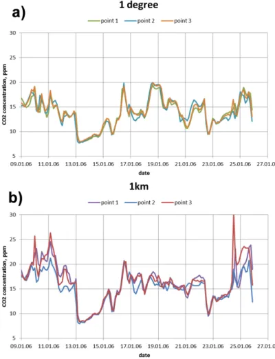
4.1 “Synthetic” test 5

To demonstrate the differences between the usage of low- and high-resolution CO2

fluxes, we performed a “synthetic” test that examined the transport of CO2around the

city of Moscow, where several large power plants are located, emitting strong plumes of CO₂that are transported to the east of the city by winds. We selected three prospective observation sites (separated from each other by∼50 km) located east of Moscow and

10

performed the calculations. The model results for the three sites are shown in Fig. 1a and b. For fluxes at a resolution of 1◦×1◦, the results are similar for all three sites. For a resolution of 1×1 km, however, the results differ among the sites, clearly showing the impact of the plumes. We note that this case study serves to demonstrate the effect of flux resolution on the model results; observation data are not available from these sites

15

for verification of the results.

4.2 Comparison of simulated concentrations at continuous monitoring stations

To demonstrate the feasibility and advantage of very-high-resolution tracer transport simulations using the coupled Eulerian-Lagrangian approach, we chose several contin-uous monitoring stations and performed simulations with (a) NIES-TM, (b) the coupled

20

model with 1◦×1◦fluxes and (c) the coupled model with 1×1 km fluxes.

First we present simulation results at the station Fyodorovskoye, for which we used 3-hourly samples of observations and model results for the year 2008. We performed a correlation analysis between the observed and simulated concentrations, yielding cor-relation coe_fficients of 0.40 for NIES-TM, 0.43 for the coupled model with 1◦×1◦fluxes,

25

(17)

GMDD

4, 2047–2080, 2011

model

A. Ganshin et al.

Title Page

Tables Figures

◭ ◮

Back Close

Full Screen / Esc

Discussion

P

a

per

|

Dis

cussion

P

a

per

|

Discussion

P

a

per

|

Discussio

n

P

a

per

|

outperforms the Eulerian model alone, although the overall correlations are relatively weak.

Similar results were obtained for the station at Egham, London, using hourly samples of observed and modelled concentrations for the year 2007. The correlation coefficients are 0.47 for NIES-TM, 0.54 for the coupled model with 1◦×1◦ fluxes, and 0.55 for the

5

coupled model with 1×1 km fluxes. Again, the correlations are relatively weak.

Overall, the correlations between observed and simulated concentrations are not as high as we expected, possibly because the model mixed layer depth was not accurately estimated. To investigate this possibility, we restricted our analysis to observations and model results sampled at hourly intervals in the daytime, because estimations of mixed

10

layer depth are expected to be reasonably accurate during the well-mixed daytime conditions. The data selection could also consider the wind fields and boundary layer height, but we did not perform such extensive sensitivity tests based on model mete-orology. Also usage of biospheric fluxes with daily variation constrains calculation of night-time values.

15

In the case of daytime sampling only, we see an obvious increase in the correlation coefficients between model and observations. For example, in the case of Fyodor-ovskoye, the correlation coefficients are 0.65 for NIES-TM, 0.68 for the coupled model with 1◦×1◦ fluxes, and 0.735 for the coupled model with 1×1 km fluxes. For Egham, the corresponding correlations are 0.66, 0.66, and 0.69, respectively.

20

We also compared the simulations results obtained using different duration of trajec-tories in the Lagrangian model. Using 7-day instead of 2-day trajectrajec-tories, we obtained a minor increase in the correlation coefficient from 0.735 to 0.740 for the 1×1 km fluxes at Fyodorovskoye. This improvement (by 0.005) is not statistically significant because the Fisher r-to-z transformation gives a two-tailed p-value of 0.7414, which is much

25

(18)

GMDD

4, 2047–2080, 2011

model

A. Ganshin et al.

Title Page

Tables Figures

◭ ◮

Back Close

Full Screen / Esc

Discussion

P

a

per

|

Dis

cussion

P

a

per

|

Discussion

P

a

per

|

Discussio

n

P

a

per

|

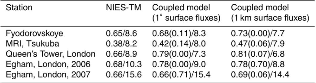
For the remaining stations, we considered only daytime sampling of observations. The results are presented in Table 3, and a Taylor diagram (Taylor, 2001) for all of the simulated stations is shown in Fig. 2a. The results show that the coupled model is su-perior to the Eulerian model alone in terms of reproducing the observations. The use of 1×1 km surface fluxes (instead of 1◦×1◦fluxes) results in a higher correlation coe_ffi

-5

cient between simulations and observations. For most of the stations considered here, the combined model and 1×1 km emissions inventory resulted in an improvement in the correlation and in the centred root-mean-square (RMS) di_fference.

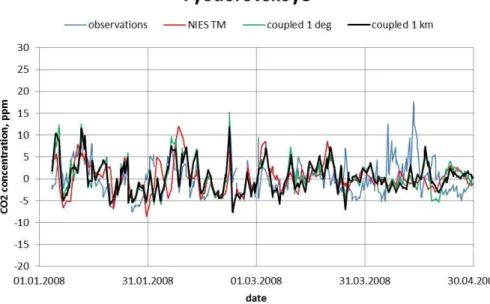
4.3 Comparison of modelled and observed high-frequency variability

The high-resolution model performs better than the low-resolution model in

represent-10

ing the high-frequency variability of observed concentrations. The skill of simulations of CO₂concentrations is a_ffected by the quality of atmospheric transport, which dom-inates the variability at the synoptic scale, and the accuracy of surface fluxes, which affects the seasonal cycle (Patra et al., 2008). Therefore, to evaluate the quality of high-resolution simulations it is advisable to separate the high-frequency synoptic-scale

vari-15

ability from the low-frequency variability related to the seasonal cycle of surface fluxes. The high-frequency variability was extracted from the observations and from the model results by employing the following equation:

Cd=Ci−

1

n+1

i+n/2

X

j=i−n/2

Cj (6)

where:Cd– de-seasonalized CO2concentration;Ci – original CO2concentration; and

20

C_j – average CO2 concentration over a 30-day period. Fifteen-day averaging was

performed at the beginning and end of the analysis period.

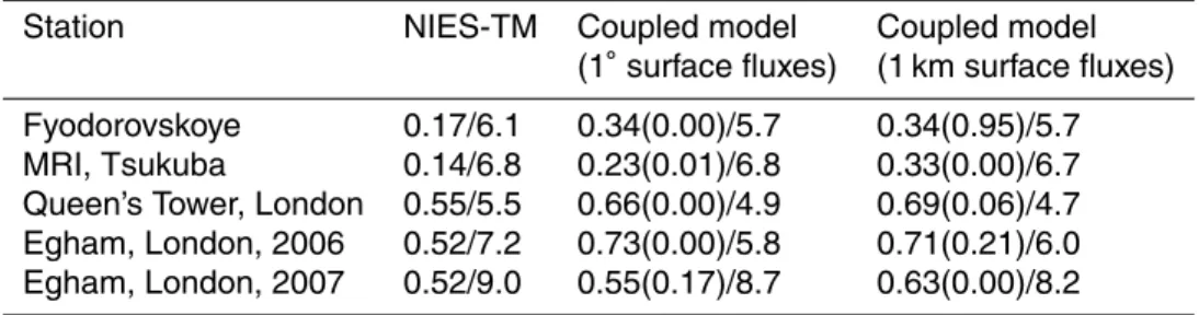
Table 4 summarizes of correlation coefficients and RMS differences. The results for individual stations are shown in Figs. 3–6 for a period of 4 months. A Taylor diagram (Taylor, 2001) is presented in Fig. 2b. The coupled model outperforms the Eulerian

(19)

GMDD

4, 2047–2080, 2011

model

A. Ganshin et al.

Title Page

Tables Figures

◭ ◮

Back Close

Full Screen / Esc

Discussion

P

a

per

|

Dis

cussion

P

a

per

|

Discussion

P

a

per

|

Discussio

n

P

a

per

|

model for all stations. The use of 1×1 km fluxes further improves the correlations and the RMS di_fferences, although in some cases there is no clear advantage over the use of 1◦×1◦fluxes. For the site at Fyodorovskoye and the MRI tower, the correlations are relatively weak for all flux resolutions, possibly due to seasonal variations (which could potentially a_ffect the total correlation).

5

5 Conclusions

We demonstrated the feasibility of a very-high-resolution tracer transport simulation with a coupled Eulerian-Lagrangian model extended to a global flux-field resolution of 1×1 km. We prepared and tested a high-resolution flux dataset and model framework, and performed simulations of atmospheric CO2 at selected observational points using

10

(a) a grid-based Eulerian transport model running at a medium resolution of 2.5◦, (b) a Lagrangian plume dispersion model and (c) surface fluxes at a resolution of 1×1 km. A comparison of modelled and observed CO2 simulations revealed that the coupled

model outperforms the Eulerian model alone. The use of surface fluxes at a resolution of 1×1 km has a clear advantage over lower-resolution (1◦×1◦) fluxes in

reproduc-15

ing the high-concentration spikes caused by anthropogenic emissions. We propose a technique to represent fluxes as a combination of fixed spatial patterns at a high resolution and temporal variability at medium resolution, thereby significantly reducing memory and computational demands. This model can be efficiently used to analyse continuous observation data for sites downwind of a large emitting source. The model

20

explicitly treats areas of sharp discontinuities in CO2 flux, such as coastlines, where

(20)

GMDD

4, 2047–2080, 2011

model

A. Ganshin et al.

Title Page

Tables Figures

◭ ◮

Back Close

Full Screen / Esc

Discussion

P

a

per

|

Dis

cussion

P

a

per

|

Discussion

P

a

per

|

Discussio

n

P

a

per

|

Acknowledgements. We thank A. Stohl for providing the FLEXPART model and the JRA-25 long-term reanalysis cooperative research project carried out by the JMA and CRIEPI. V. Val-sala is thankful for generous support by GOSAT project at NIES, Tsukuba, Japan. R. J. Andres was sponsored by the US Department of Energy, the Office of Science, and the Biological and Environmental Research (BER) program, and worked at Oak Ridge National Laboratory 5

(ORNL) under US Department of Energy contract DE-AC05-00OR22725.

References

Andres, R. J., Gregg, J. S., Marland, G., and Boden, T. A.: Monthly, global emissions of carbon dioxide from fossil fuel consumption, Tellus B, 63(3), 309–327, 2011.

Belikov, D., Maksyutov, S., Miyasaka, T., Saeki, T., Zhuravlev, R., and Kiryushov, B.: Mass-10

conserving tracer transport modelling on a reduced latitude-longitude grid with NIES-TM, Geosci. Model Dev., 4, 207–222, doi:10.5194/gmd-4-207-2011, 2011.

BP: Statistical Review of World Energy, London, available at: http://www.bp.com/ productlanding.do?categoryId=6929&contentId=7044622 (last access: 23 August 2010), 2008.

15

Buell, C. E.: The structure of two-point wind correlations in the atmosphere, J. Geophys. Res., 65(10), 3353–3366, 1960.

Buell, C. E.: Correlation functions for wind and geopotential on isobaric surfaces, J. Appl. Meteor., 11, 51–59, 1972.

Core Writing Team: Pachauri, R. K. and Reisinger, A. (Eds.): IPCC Fourth Assessment Report 20

(AR4): Climate Change 2007: Synthesis Report: Contribution of Working Groups I, II and III to the Fourth Assessment Report of the Intergovernmental Panel on Climate Change, IPCC, Geneva, Switzerland, 104, 2007.

Folini, D., Ubl, S., and Kaufmann, P.: Lagrangian particle dispersion modeling for the high Alpine site Jungfraujoch, J. Geophys. Res., 113, D18111, doi:10.1029/2007JD009558, 2008. 25

(21)

GMDD

4, 2047–2080, 2011

model

A. Ganshin et al.

Title Page

Tables Figures

◭ ◮

Back Close

Full Screen / Esc

Discussion

P

a

per

|

Dis

cussion

P

a

per

|

Discussion

P

a

per

|

Discussio

n

P

a

per

|

Gandin, L. S.: Objective analysis of meteorological fields, Translation US Dep. Commerce, Springfield, Va., 242 pp., 1965.

Gloor, M., Bakwin, P., Hurst, D., Lock, L., Draxler, R., and Tans P.: What is the concentration footprint of a tall tower?, J. Geophys. Res., 106(D16), 17831–17840, 2001.

Gourdji, S. M., Hirsch, A. I., Mueller, K. L., Yadav, V., Andrews, A. E., and Michalak, A. M.: 5

Regional-scale geostatistical inverse modeling of North American CO₂ fluxes: a synthetic data study, Atmos. Chem. Phys., 10, 6151–6167, doi:10.5194/acp-10-6151-2010, 2010. Gurney, K. R., Law, R. M., Denning, A. S., Rayner, P. J., Baker, D., Bousquet, P., Bruhwiler, L.,

Chen, Y.-H., Ciais, P., Fan, S., Fung, I. Y., Gloor, M., Heimann, M., Higuchi, K., John, J., Maki, T., Maksyutov, S., Masarie, K., Peylin, P., Prather, M., Pak, B. C., Randerson, J., Sarmiento, 10

J., Taguchi, S., Takahashi, T., and Yuen, C.-W.: Towards robust regional estimates of CO₂ sources and sinks using atmospheric transport models, Nature, 415, 626–630, 2002. Gurney, K. R., Scott Denning, A., Rayner, P., Pak, B., Baker, D., Bousquet, P., Bruhwiler, L.,

Chen, Y.-H., Ciais, P., Fung, I. Y., Heimann, M., Higuchi, K., John, J., Maki, T., Maksyutov, S., Peylin, P., Prather, M., and Taguchi, S.: Transcom 3 inversion intercomparison: Model 15

mean results for the estimation of seasonal carbon sources and sinks, Global Biogeochem. Cy., 18, GB1010, doi:10.1029/2003GB002111, 2004.

Holzer, M. and Hall, T. M.: Transit-time and tracer-age distributions in geophysical flows, J. Atmos. Sci., 57, 3539–3558, 2000.

Inoue, H. Y. and Matsueda, H.: Variations in atmospheric CO2 at the Meteorological Research 20

Institute, Tsukuba, Japan, J. Atmos. Chem., 23, 137–161, 1996.

Inoue, H. Y. and Matsueda, H.: Measurements of atmospheric CO₂from a meteorological tower in Tsukuba, Japan, Tellus, 53B, 205–219, 2001.

Ishii, M., Saito, S., Tokieda, T., Kawano, T., Matsumoto, K., and Yoshikawa-Inoue, H.: Variability of Surface Layer CO₂ Parameters in the Western and Central Equatorial Pacific, Global 25

Environmental Changes in the Ocean and on Land, 59–94, 2004.

Ito, A., Inatomi, M., Mo, W., Lee, M., Koizumi, H., Saigusa, N., Murayama, S., and Yamamoto, S.: Examination of model-estimated ecosystem respiration by use of flux measurement data from a cool-temperate deciduous broad-leaved forest in central Japan, Tellus B, 59, 616–624, 2007.

30

(22)

GMDD

4, 2047–2080, 2011

model

A. Ganshin et al.

Title Page

Tables Figures

◭ ◮

Back Close

Full Screen / Esc

Discussion

P

a

per

|

Dis

cussion

P

a

per

|

Discussion

P

a

per

|

Discussio

n

P

a

per

|

Kurbatova, J., Li, C., Varlagin, A., Xiao, X., and Vygodskaya, N.: Modeling carbon dynamics in two adjacent spruce forests with different soil conditions in Russia, Biogeosciences, 5, 969–980, doi:10.5194/bg-5-969-2008, 2008.

Lin, J. C., Gerbig, C., Wofsy, S. C., Andrews, A. E., Daube, B. C., Davis, K. J., and Grainger, C. A.: A near-field tool for simulating the upstream influence of atmospheric observations: The 5

Stochastic Time-Inverted Lagrangian Transport (STILT) model, J. Geophys. Res., 108(D16), 4493, doi:10.1029/2002JD003161, 2003.

Lin, J. C., Brunner, D., and Gerbig, C.: Studying Atmospheric Transport Through Lagrangian Models, EOS, 92(21), 177–184, 2011.

Maksyutov, S., Patra, P. K., Onishi, R., Saeki, T., and Nakazawa, T.: NIES/FRCGC Global At-10

mospheric Tracer Transport Model: Description, Validation, and Surface Sources and Sinks Inversion, J. Earth Simul., 9, 3–18, 2008.

Milyukova, I. M., Kolle, O., Varlagin, A. V., Vygodskaya, N. N., Schulze, E. D., and Lloyd, J.: Carbon balance of a southern taiga spruce stand in european Russia, Tellus B, 54, 429–442, 2002.

15

Nakatsuka, Y. and Maksyutov, S.: Optimization of the seasonal cycles of simulated CO2 flux by fitting simulated atmospheric CO₂to observed vertical profiles, Biogeosciences, 6, 2733– 2741, doi:10.5194/bg-6-2733-2009, 2009.

Nehrkorn, T., Eluszkiewicz, J., Wofsy, S. C., Lin, J. C., Gerbig, C., Longo, M., and Freitas, S.: Coupled weather research and forecasting-stochastic time-inverted lagrangian transport 20

(WRF–STILT) model, Meteorol. Atmos. Phys., 107(1–2), 51–64, doi:10.1007/s00703-010-0068-x, 2010.

Oda, T. and Maksyutov, S.: A very high-resolution (1 km×1 km) global fossil fuel CO₂emission inventory derived using a point source database and satellite observations of nighttime lights, Atmos. Chem. Phys., 11, 543–556, doi:10.5194/acp-11-543-2011, 2011.

25

Onogi, K., Tsutsui, J., Koide, H., Sakamoto, M., Kobayashi, S., Hatsushika, H., Matsumoto, T., Yamazaki, N., Kamahori, H., Takahashi, K., Kadokura, S., Wada, K., Kato, K., Oyama, R., Ose, T., Mannoji, N., and Taira, R.: The JRA-25 Reanalysis, J. Meteor. Soc. Japan, 85, 369–432, 2007.

Patra, P. K., Law, R. M., Peters, W., Rodenbeck, C., Takigawa, M., Aulagnier, C., Baker, I., 30

(23)

GMDD

4, 2047–2080, 2011

model

A. Ganshin et al.

Title Page

Tables Figures

◭ ◮

Back Close

Full Screen / Esc

Discussion

P

a

per

|

Dis

cussion

P

a

per

|

Discussion

P

a

per

|

Discussio

n

P

a

per

|

Y., Onishi, R., Parazoo, N., Pieterse, G., River, L., Satoh, M., Serrar, S., Taguchi, S., Vautard, R., Vermeulen, A. T., and Zhu, Z.: TransCom model simulations of hourly atmospheric CO₂: Analysis of synoptic-scale variations for the period 2002–2003, Global Biogeochem. Cy., 22, GB4013, doi:10.1029/2007GB003081, 2008.

Richtmyer, R. D. and Morton, K. W.: Difference Methods for Initial-Value Problems, 2nd Edn., 5

Wiley-Interscience, 1967.

Rigby, M., Manning, A. J., and Prinn, R. G.: Inversion of long-lived trace gas emissions using combined Eulerian and Lagrangian chemical transport models, Atmos. Chem. Phys. Dis-cuss., 11, 14689–14717, doi:10.5194/acpd-11-14689-2011, 2011.

Rigby, M., Toumi, R., Fisher, R., Lowry, D., and Nisbet, E. G.: First continuous measurements 10

of CO₂ mixing ratio in central London using a compact diffusion probe, Atmos. Environ, 42, 8943–8953, 2008.

R ¨odenbeck, C., Gerbig, C., Trusilova, K., and Heimann, M.: A two-step scheme for high-resolution regional atmospheric trace gas inversions based on independent models, Atmos. Chem. Phys., 9, 5331–5342, doi:10.5194/acp-9-5331-2009, 2009.

15

Saito, M., Ito, A., and Maksyutov, S.: Evaluation of Biases in JRA-25/JCDAS precipita-tion and their Impact on the Global Terrestrial Carbon Balance, J. Clim., 21, 4109–4125, doi:10.1175/2011JCLI3918.1, 2011.

Seibert, P. and Frank, A.: Source-receptor matrix calculation with a Lagrangian particle disper-sion model in backward mode, Atmos. Chem. Phys., 4, 51–63, doi:10.5194/acp-4-51-2004, 20

2004.

Seibert, P., Kromp-Kolb, H., Baltensperger, U., Jost, D.T., Schwikowski, M., Kasper, A., and Puxbaum, H.: Trajectory analysis of aerosol measurements at high Alpine sites, edited by: Borrell, P M., Borrell, P., Cvitas, T., and Seiler, W., Proceedings of the EUROTRAC Sympo-sium ’94 SPB Academic Publishing, Hague, 1283, 689–693, 1994.

25

Stohl, A.: Trajectory statistics – a new method to establish source-receptor relationships of air pollutants and its application to the transport of particulate sulphate in Europe, Atmos. Environ., 30, 579-587, 1996.

Stohl, A.: Computation, accuracy and applications of trajectories – review and bibliography, Atmos. Environ., 32(6), 947–966, 1998.

30

(24)

GMDD

4, 2047–2080, 2011

model

A. Ganshin et al.

Title Page

Tables Figures

◭ ◮

Back Close

Full Screen / Esc

Discussion

P

a

per

|

Dis

cussion

P

a

per

|

Discussion

P

a

per

|

Discussio

n

P

a

per

|

Taylor, K. E.: Summarizing multiple aspects of model performance in a single diagram, J. Geophys. Res., 106, 7183–7192, 2001.

Tewarson, R. P.: Sparse matrices, Academic Press, 1973.

Trusilova, K., R ¨odenbeck, C., Gerbig, C., and Heimann, M.: Technical Note: A new coupled system for global-to-regional downscaling of CO₂ concentration estimation, Atmos. Chem. 5

Phys., 10, 3205–3213, doi:10.5194/acp-10-3205-2010, 2010.

(25)

GMDD

4, 2047–2080, 2011

model

A. Ganshin et al.

Title Page

Tables Figures

◭ ◮

Back Close

Full Screen / Esc

Discussion

P

a

per

|

Dis

cussion

P

a

per

|

Discussion

P

a

per

|

Discussio

n

P

a

per

|

Table 1.Combinations of emissions analysed in this study.

Type of High Low

emissions resolution resolution

Fossil fuel 1 annual file with a resolution of 1×1 km for spatial representation

12 monthly files with a resolution of 1◦×1◦for temporal variations Biosphere Global vegetation map

(15 biotypes) with a resolution of 1×1 km for spatial representation

Fluxes with a spatial

resolution of 0.5◦×0.5◦and a temporal resolution of 1 day for each biotype

Ocean Sea-land mask derived from a

global vegetation map for the biosphere with a resolution of 1×1 km for reconstruction of the coastline

(26)

GMDD

4, 2047–2080, 2011

model

A. Ganshin et al.

Title Page

Tables Figures

◭ ◮

Back Close

Full Screen / Esc

Discussion

P

a

per

|

Dis

cussion

P

a

per

|

Discussion

P

a

per

|

Discussio

n

P

a

per

|

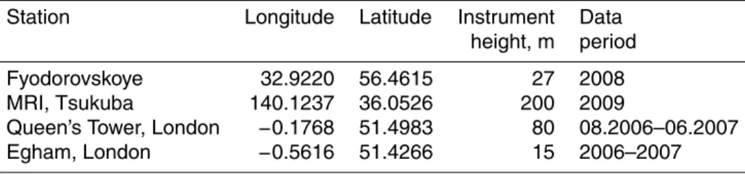
Table 2.General information on the stations.

Station Longitude Latitude Instrument Data

height, m period

Fyodorovskoye 32.9220 56.4615 27 2008

MRI, Tsukuba 140.1237 36.0526 200 2009

Queen’s Tower, London −0.1768 51.4983 80 08.2006–06.2007

(27)

GMDD

4, 2047–2080, 2011

model

A. Ganshin et al.

Title Page

Tables Figures

◭ ◮

Back Close

Full Screen / Esc

Discussion

P

a

per

|

Dis

cussion

P

a

per

|

Discussion

P

a

per

|

Discussio

n

P

a

per

|

Table 3. Information on correlation coefficients (statistical significance between correlation coefficients (for 1◦: comparison between NIES-TM and 1◦; for 1 km: comparison between 1◦ and 1 km) and two-tailed p-value between current and previous (from the cell to the left of the current cell in table) correlation coefficients)/centred root-mean-square difference between simulations and observations.

Station NIES-TM Coupled model Coupled model

(1◦surface fluxes) (1 km surface fluxes)

Fyodorovskoye 0.65/8.6 0.68(0.11)/8.3 0.73(0.00)/7.7

MRI, Tsukuba 0.38/8.2 0.42(0.14)/8.0 0.47(0.06)/7.9

Queen’s Tower, London 0.66/8.9 0.79(0.00)/7.3 0.81(0.07)/6.8

Egham, London, 2006 0.68/10.3 0.78(0.00)/9.0 0.78(0.70)/8.8

(28)

GMDD

4, 2047–2080, 2011

model

A. Ganshin et al.

Title Page

Tables Figures

◭ ◮

Back Close

Full Screen / Esc

Discussion

P

a

per

|

Dis

cussion

P

a

per

|

Discussion

P

a

per

|

Discussio

n

P

a

per

|

Table 4. Information on correlation coefficients (statistical significance between correlation coefficients (for 1◦: comparison between NIES-TM and 1◦; for 1 km: comparison between 1◦ and 1 km) and two-tailed p-value between current and previous (from the cell to the left of the current cell in table) correlation coefficients)/centred root-mean-square difference between simulations and observations. The results have been deseasonalized.

Station NIES-TM Coupled model Coupled model

(1◦ surface fluxes) (1 km surface fluxes)

Fyodorovskoye 0.17/6.1 0.34(0.00)/5.7 0.34(0.95)/5.7

MRI, Tsukuba 0.14/6.8 0.23(0.01)/6.8 0.33(0.00)/6.7

Queen’s Tower, London 0.55/5.5 0.66(0.00)/4.9 0.69(0.06)/4.7

Egham, London, 2006 0.52/7.2 0.73(0.00)/5.8 0.71(0.21)/6.0

(29)

GMDD

4, 2047–2080, 2011

model

A. Ganshin et al.

Title Page

Tables Figures

◭ ◮

Back Close

Full Screen / Esc

Discussion

P

a

per

|

Dis

cussion

P

a

per

|

Discussion

P

a

per

|

Discussio

n

P

a

per

|

Fig. 1.Results for three imaginary observation sites located east of Moscow.(a)1◦resolution;

(30)

GMDD

4, 2047–2080, 2011

model

A. Ganshin et al.

Title Page

Tables Figures

◭ ◮

Back Close

Full Screen / Esc

Discussion

P

a

per

|

Dis

cussion

P

a

per

|

Discussion

P

a

per

|

Discussio

n

P

a

per

|

(31)

GMDD

4, 2047–2080, 2011

model

A. Ganshin et al.

Title Page

Tables Figures

◭ ◮

Back Close

Full Screen / Esc

Discussion

P

a

per

|

Dis

cussion

P

a

per

|

Discussion

P

a

per

|

Discussio

n

P

a

per

|

(32)

GMDD

4, 2047–2080, 2011

model

A. Ganshin et al.

Title Page

Tables Figures

◭ ◮

Back Close

Full Screen / Esc

Discussion

P

a

per

|

Dis

cussion

P

a

per

|

Discussion

P

a

per

|

Discussio

n

P

a

per

|

(33)

GMDD

4, 2047–2080, 2011

model

A. Ganshin et al.

Title Page

Tables Figures

◭ ◮

Back Close

Full Screen / Esc

Discussion

P

a

per

|

Dis

cussion

P

a

per

|

Discussion

P

a

per

|

Discussio

n

P

a

per

|

(34)

GMDD

4, 2047–2080, 2011

model

A. Ganshin et al.

Title Page

Tables Figures

◭ ◮

Back Close

Full Screen / Esc

Discussion

P

a

per

|

Dis

cussion

P

a

per

|

Discussion

P

a

per

|

Discussio

n

P

a

per

|