www.atmos-chem-phys.net/10/4403/2010/ doi:10.5194/acp-10-4403-2010
© Author(s) 2010. CC Attribution 3.0 License.
Chemistry
and Physics
Observed and simulated global distribution and budget of
atmospheric C
2
-C
5
alkanes
A. Pozzer1,2, J. Pollmann2, D. Taraborrelli2, P. J¨ockel2,*, D. Helmig3, P. Tans4, J. Hueber3, and J. Lelieveld1,2 1The Cyprus Institute, Energy, Environment and Water Research Center, P. O. Box 27456, 1645 Nicosia, Cyprus 2Air Chemistry Department, Max-Planck Institute of Chemistry, P. O. Box 3060, 55020 Mainz, Germany 3Institute of Arctic and Alpine Research (INSTAAR), University of Colorado, UCB 450, CO 80309, USA 4NOAA/ESRL, 325 Broadway, Boulder, CO 80303, USA
*now at: DLR, Institut fuer Physik der Atmosphaere, Oberpfaffenhofen, 82234 Wessling, Germany Received: 7 December 2009 – Published in Atmos. Chem. Phys. Discuss.: 13 January 2010 Revised: 23 April 2010 – Accepted: 26 April 2010 – Published: 12 May 2010
Abstract. The primary sources and atmospheric chemistry of C2-C5 alkanes were incorporated into the atmospheric chemistry general circulation model EMAC. Model output is compared with new observations from the NOAA/ESRL GMD Cooperative Air Sampling Network. Based on the global coverage of the data, two different anthropogenic emission datasets for C4-C5alkanes, widely used in the mod-elling community, are evaluated. We show that the model reproduces the main atmospheric features of the C2-C5 alka-nes (e.g., seasonality). While the simulated values for ethane and propane are within a 20% range of the measurements, larger deviations are found for the other tracers. Accord-ing to the analysis, an oceanic source of butanes and pen-tanes larger than the current estimates would be necessary to match the observations at some coastal stations. Finally the effect of C2-C5alkanes on the concentration of acetone and acetaldehyde are assessed. Their chemical sources are largely controlled by the reaction with OH, while the reac-tions with NO3and Cl contribute only to a little extent. The total amount of acetone produced by propane,i-butane and
i-pentane oxidation is 11.2 Tg/yr, 4.3 Tg/yr, and 5.8 Tg/yr, respectively. Moreover, 18.1, 3.1, 3.4, 1.4 and 4.8 Tg/yr of acetaldehyde are formed by the oxidation of ethane, propane,
n-butane,n-pentane andi-pentane, respectively.
Correspondence to:A. Pozzer ([email protected])
1 Introduction
Non Methane Hydrocarbons (NMHC) play an important role in tropospheric chemistry and ozone formation. They sig-nificantly influence the hydroxyl radical HOx (=OH+HO2) budget through many complex reaction cycles (Logan, 1985; Houweling et al., 1998; Seinfeld and Pandis, 1997; Atkinson, 2000). For example, NMHC are precursors of the formation of oxygenated volatile organic compounds (OVOC) such as acetone, formaldehyde and acetaldehyde. The seasonal and spatial distribution of NMHC is determined by:
– emission strength (Singh et al., 2001, 2003; Singh and Zimmermann, 1992),
– photochemical reactions (Cardelino and Chameides, 1990; Singh et al., 1995; Neeb, 2000),
– atmospheric transport (Rood, 1987; Brunner et al., 2003),
– dilution due to atmospheric mixing (Roberts et al., 1985; Parrish et al., 2007).
4404 A. Pozzer et al.: Atmospheric C2-C5alkanes remote locations across the globe during the years 2005–
2008. The NMHC flask measurements (Pollmann et al., 2008) include ethane (C2H4), propane (C3H8), butane (or
n-butane, n-C4H10), isobutane (ori-butane, i-C4H10), pen-tane (orn-pentane, n-C5H12) and isopentane (ori-pentane, i-C5H12).
In Sect. 2 the model is presented: two simulations (E1 and E2), based on two different emission databases for butanes (i.e.n-butane plusi-butane) and pentanes (i.e.n-pentane plus
i-pentane), are described. Then, the observational data set (Sect. 3) is described, followed by a comparison between model results and observations (Sect. 4). Finally, we discuss the contribution of C2-C5alkanes to the atmospheric produc-tion and mixing ratios of the most important OVOC (Sect. 5), with a focus on the acetone budget.
2 Model description and setup
EMAC is a combination of the general circulation model ECHAM5 (Roeckner et al., 2006) (version 5.3.01) and the Modular Earth Submodel System (MESSy, version 1.1, J¨ockel et al., 2005). Descriptions of the model system were published by J¨ockel et al. (2006) and Pozzer et al. (2007). Details about the model system can be found at http://www.messy-interface.org. The setup is based on that of the evaluation simulation S1, described by J¨ockel et al. (2006). It was modified by adding the emissions of butane and pentane isomers, and their corresponding oxidation path-ways (see Sect. 2.1 and Sect. 2.2).
The simulation period covers the years 2005–2008, plus two additional months of spin-up time. The initial conditions are taken from the evaluation simulation S1 of the model. Dry and wet deposition processes are described by Kerk-weg et al. (2006a) and Tost et al. (2006), respectively; the tracer emissions are described by Kerkweg et al. (2006b). As in the simulation S1, the applied spectral truncation of the ECHAM5 base model is T42, corresponding to an horizontal resolution of≈2.8◦×2.8◦of the quadratic Gaussian grid.
The applied vertical resolution is 90 layers, with about 25 levels in the troposphere. The model setup includes feed-backs between chemistry and dynamics via radiation calcu-lations. The model dynamics was weakly nudged (Jeuken et al., 1996; J¨ockel et al., 2006; Lelieveld et al., 2007) to-wards the analysis data of the ECMWF (European Center Medium-range Weather Forecast) operational model (up to 100 hPa) to realistically represent the tropospheric meteo-rology of the selected period. This implies that the gen-eral circulation model is following the meteorology (at syn-optic scale) as assimilated by the ECMWF analysis, which takes advantage of more than 75 million observations in a 12 h period (98% of them are from satellites). We refer to the ECMWF (http://www.ecmwf.int) for further information. The uncertainties connected with the weak nudging (or bet-ter, due to the internal variability of the model which remains
despite the nudging) can be estimated by the differences of meteorological parameters between the two simulations. This has already been discussed in a previous study (Pozzer et al., 2009), where differences of∼15% were found between two different simulations for temperature and relative humid-ity. It must be stressed, however, that the usage of monthly averages drastically decreases the uncertainties arising from the differences in the meteorology. As estimated by Pozzer et al. (2009), the differences in the temperature and relative humidity are below 5% if monthly averages are considered. It is hence expected to reproduce the meteorology assimi-lated by the ECMWF analysis, allowing a direct compari-son of model results with observations. Nevertheless, for the overall representation of the real meteorology, we rely on the ECMWF data assimilation, which has been evaluated previ-ously (see for example Bozzano et al. (2004) or Salstein et al. (2008) for comparisons with surface observations). Follow-ing Bozzano et al. (2004), for temperature, pressure and hu-midity, a low relative difference between ECMWF analysis data and measurements is observed, while for the wind speed a relative difference of up to 100% was determined from the comparison of model output and observations. These un-certainties do not translate directly into unun-certainties in the simulated alkane mixing ratios, due to the non-linearity of the system. In addition, errors in estimating different meteo-rological parameters have different direct/indirect effects on the simulated chemistry of alkanes. Nevertheless, Bozzano et al. (2004) also showed that when long time averages are considered (as in this study), the differences are much lower. Therefore an upper threshold of∼100% is estimated for the uncertainty in the simulated alkane concentrations.
2.1 Chemistry
The chemical kinetics within each grid-box was calculated with the submodel MECCA (Sander et al., 2005). The set of chemical equations solved by the Kinetic PreProcessor (KPP, Damian et al. (2002); Sandu et al. (2003); Daescu et al. (2003), see http://people.cs.vt.edu/∼asandu/Software/Kpp/)
in this study was essentially the same as in J¨ockel et al. (2006). However, the propane oxidation mechanism (which was already included in the original chemical mechanism) was slightly changed, and new reactions for the butane and pentane isomers were added.
This substitution includes the production of corresponding amounts of a model peroxy radical (RO2), which has generic properties representing the total number of RO2 produced during the “instantaneous oxidation”. With this approach we take into account the NO→NO2conversions and the HO2 →OH interconversion. It is assumed that the reactions with OH and NO3 have the same product distribution. The Cl distribution was nudged with monthly average mixing ratios taken from Kerkweg et al. (2008a,b, and references therein). Thus, both alkanes and Cl are simulated without the need of a computationally expensive chemical mechanism. Small uncertainties in the model simulation have to be attributed to the reaction rates used in this study. Nevertheless, accord-ing to the IUPAC (International Union of Pure and Applied Chemistry) recommendation for butanes and pentanes, the uncertainties in the reaction rates are on the order of 7%. Moreover, the chemical mechanism itself does not increase the uncertainties in the simulation of C4-C5alkanes, but only those of their products, due to the simplified degradation re-actions.
Finally, the OH concentration is very important for a cor-rect simulation of NMHC. J¨ockel et al. (2006) performed a detailed evaluation of the simulated OH abundance. In sum-mary, OH compared very well with that of other models of similar complexity. Compared to Spivakovsky et al. (2000), the EMAC simulation of OH indicated slightly higher values in the lower troposphere and lower values in the upper tropo-sphere. We refer to J¨ockel et al. (2006) for further details. 2.2 Emissions
2.2.1 Anthropogenic emissions
As pointed out by Jobson et al. (1994) and Poisson et al. (2000), the seasonal change in the anthropogenic emissions of NMHC are thought to be small, due to their relatively con-stant release from fossil fuel combustion and leakage from oil and natural gas production (Middleton et al., 1990; Blake and Rowland, 1995; Friedrich and Obermeier, 1999). The most detailed global emission inventory available is EDGAR (Olivier et al., 1999, 1996; van Aardenne et al., 2001), Emis-sion Database for Global Atmospheric Research, which was applied for the evaluation simulations of EMAC (J¨ockel et al., 2006).
In the evaluation simulation “S1” of the model (J¨ockel et al., 2006), the anthropogenic emissions were taken from the EDGAR database (version 3.2 “fast-track”, van Aardenne et al., 2005) for the year 2000. In order to keep the tions as consistent as possible with the evaluation simula-tion S1, the ethane and propane emissions were not changed and annual global emissions of 9.2 and 10.5 Tg/yr respec-tively, as reported by Pozzer et al. (2007), were applied. Furthermore, the total butanes and pentanes emissions from EDGARv2.0 were used, i.e. 14.1 Tg/yr and 12.3 Tg/yr, re-spectively. The simulation with these emissions for butanes
Fig. 1. i-butane versus butanes (upper figure) andi-pentane ver-sus pentanes (lower figure) measurements in pmol/mol. The black line represents the 1 to 1 line, while the red line represent the lin-ear regression of the data. In the upper left corner the regression parameters are presented. Note the logarithmic scale of the axes.
and pentanes is further denoted as “E1”. Based on speciation factors described below, the total emissions are 9.9 Tg/yr for
n-butane (70% of all butanes), 4.2 Tg/yr fori-butane (30% of all butanes), 4.3 Tg/yr forn-pentane (35% of all pentanes) and 8.0 Tg/yr fori-pentane (65% of all pentanes).
4406 A. Pozzer et al.: Atmospheric C2-C5alkanes
Table 1.Summary of the emissions used in simulation S1, E1 and E2 in Tg(species)/yr.
simulation emission type C2H6 C3H8 n-C4H10 i-C4H10 n-C5H12 i-C5H12 higher alkanes
S1 anthropogenic 9.2b 10.5b – – – – 73.7
biomass burning 2.8e 0.9e – – – – 1.1
oceanic 0.5d 0.3d – – – – 0.4
E1 anthropogenic 9.2b 10.5b 9.9c 4.2c 4.3c 8.0c 47.3
biomass burning 2.8e 0.9e – – – – 1.1
oceanic 0.5d 0.3d – – – – 0.4
E2 anthropogenic 9.2b 10.5b 10.1a 4.3a 4.3a 8.0a 46.9
biomass burning 2.8e 0.9e – – – – 1.1
oceanic 0.5d 0.3d – – – – 0.4
awith emissions distribution from Bey et al. (2001); bbased on EDGARv3.2, fast-track 2000;
cbased on EDGARv2.0;
dbased on Plass-D¨ulmer et al. (1995);
ebased on Van der Werf et al. (2004) and Andreae and Merlet (2001) for the year 2000 (see Sect. 2.2.2).
emissions used in simulation E2 is the one estimated by Ja-cob et al. (2002). Differently, for pentanes, the total emission estimated by Jacob et al. (2002) significantly underestimates the observed mixing ratios of these tracers in a sensitivity simulation (not shown). Hence, the total amount of pentanes used in simulation E2 was scaled to 12.3 Tg/yr, the same to-tal amount of the EDGARv2.0 database. In conclusion, the total amounts emitted in simulation E2 are 10.35, 4.35, 4.3, 8.0 Tg/yr forn-butane,i-butane,n-pentane andi-pentane, re-spectively. The emissions used in simulation S1, E1 and E2 are summarized in Table 1. The two emission sets, although with very similar total emissions of butanes and pentanes, present very different spatial distributions. The differences in a single grid box can be up to a factor of 4, depending on the location.
The speciacion fractions used fori-butane (30%) and n -butane (70%), and fori-pentane (65%) andn-pentane (35%) are from the calculation of Saito et al. (2000) and Goldan et al. (2000), respectively. These fractions have been con-firmed by McLaren et al. (1996), who showed that the ra-tio ofn-pentane toi-pentane is 0.5 (i.e. a fraction of∼66% fori-pentane and∼34% forn-pentane over pentanes). The long-term measurements from the NOAA flask data set also confirm these speciacion factors. Measurements from the database are shown in Fig. 1, with the exception of data with very high uncertainties, i.e. observations of mixing ra-tios lower than 1 pmol/mol or larger than 1000 pmol/mol. As shown in Fig. 1, the fraction ofi-butane of the butanes is∼0.33, while the fraction ofi-pentane of the pentanes is ∼0.65. These values are in close agreement with the specia-cion factors present in the literature.
2.2.2 Biomass burning
Biomass burning is a large source of ethane and propane, and a negligible source of butane and pentane isomers (An-dreae and Merlet, 2001; Guenther et al., 2000). Blake et al. (1993) extrapolated the total emission from biomass burning of 1.5 Tg/yr for ethane, and 0.6 Tg/yr for propane. Rudolph (1995) suggested instead 6.4 Tg/yr for ethane. The biomass burning contribution was added using the Global Fire Emis-sions Database (GFED version 1, Van der Werf et al., 2004) for the year 2000 (neglecting interannual variability) scaled with different emissions factors (Andreae and Merlet, 2001; von Kuhlmann et al., 2003a). The total amounts calculated are 2.76 Tg/yr and 0.86 Tg/yr for ethane and propane, re-spectively. No biomass burning emission was included for C4-C5alkanes, due to small contribution to the global bud-get of these tracers.
2.2.3 Biogenic emissions
Biogenic sources of C2-C5 alkanes appear to be negligibly small (Kesselmeier and Staudt, 1999; Guenther et al., 1995). Other measurements in rural environments (Jobson et al., 1994; Goldan et al., 1995) show no evidence of biogenic emissions of saturated C2-C5NMHC.
2.2.4 Oceanic emissions
While oceanic emissions for ethane and propane were in-cluded in this study, oceanic emissions of higher alkanes were neglected due to their small contribution and largely unknown spatio-temporal distribution.
2.2.5 Other sources
Etiope and Ciccioli (2009) proposed a geophysical (volcanic) source of ethane and propane. Based on observations of gas emissions from volcanoes, they estimated emissions of 2 to 4 Tg/yr for ethane and of 1 to 2.4 Tg/yr for propane. How-ever, since the emission distribution is unknown, it is not yet feasible to include this source into the model. In addition, re-sults from our simulations do not support a further increase in the emissions of these species (see below, Sects. 4.1–4.2).
3 Observations
The NOAA ESRL GMD (National Oceanic and Atmospheric Administration, Earth System Research Laboratory, Global Monitoring Division, Boulder, CO, USA) cooperative air sampling network currently includes 59 active surface sam-pling stations, where usually one pair of flask samples is col-lected every week. This network is the most extensive global flask sampling network in operation, both in terms of number of sites and total number of samples collected. NMHC data are available from approximately 40 of these sampling sta-tions (see http://www.esrl.noaa.gov/gmd/), covering the lat-itudes from 82◦N (ALT, Alert, Canada) to 89.98◦S (SPO,
South Pole). However, the measurements collected from the stations are not homogeneously distributed in time and some gaps are present in the data. A variable number of measurements were used to calculate the monthly averages here. The monthly variability was calculated as the monthly standard deviation of the measurements. As pointed out by Haas-Laursen and Hartley (1997), these flask samples have been collected under non-polluted conditions, i.e., for sta-tions close to local sources only certain wind direcsta-tions were selected to avoid local contamination. Moreover, most of the stations are in remote regions, where background condi-tions are sampled. It is hence expected that the model resolu-tion used in this study is sufficient to reproduce the chemical history of the C2-C5alkanes, while higher resolution simu-lations would be required for studying specific stations, as example in industrialized areas or where sporadic biomass burning emissions are important (see below Sect. 4.7).
A detailed description of the flask instrument and a full evaluation of the analytical technique was published by (Poll-mann et al., 2008). An intercomparison with the WMO GAW (World Meteorological Organization, Global Atmospheric Watch) station in Hohenpeissenberg, Germany showed that flask measurements meet the WMO data quality objective (World Meteorological Organization, 2007). These find-ings were confirmed during a recent audit by the World
Calibration Center for Volatile Organic Compound (WCC-VOC, http://imk-ifu.fzk.de/wcc-voc/).
4 Comparison of the model results with observations
In this section only time series from a selected num-ber of sites are presented. The complete set of fig-ures can be found in the electronic supplement of this paper (see http://www.atmos-chem-phys.net/10/4403/2010/ acp-10-4403-2010-supplement.pdf).
The seasonal cycle of NMHC exhibits a maximum corre-sponding to the local winter and a minimum correcorre-sponding to the local summer, confirming previous studies by Gautrois et al. (2003); Lee et al. (2006); Swanson et al. (2003). In fact, Hagerman et al. (1997) and Sharma et al. (2000) showed that the seasonal cycle of C2-C5 alkanes is anti-correlated with the production rate of the main atmospheric oxidant (OH, see Spivakovsky et al., 2000; J¨ockel et al., 2006). The flask measurements used in this study confirm this and the model is able to reproduce the observed seasonal signal, with high mixing ratios during winter and low mixing ratios during summer. In addition, due to the small contribution of C4-C5 alkanes to the total OH sink (less than∼10%), both simula-tions E1 and E2, reproduce the OH mixing ratios simulated in the reference simulation S1, with local instantaneous dif-ferences below∼15%. When monthly averages are consid-ered for OH, the maximum differences between simulation S1 and simulation E1 are below∼5%, while the differences between simulation E1 and simulation E2 are below∼2%. For ethane and propane, the same sources (emissions), sinks (OH) and transport (thanks to the nudging) are then applied in both simulations E1 and E2. Although the results for these two tracers are not binary identical in the two simulations, they show only negligible differences, which are not statisti-cally significant. Hence, for ethane and propane, only results from the simulation E1 are shown. On contrary, results from both simulations are presented for butanes and pentanes.
4408 A. Pozzer et al.: Atmospheric C2-C5alkanes
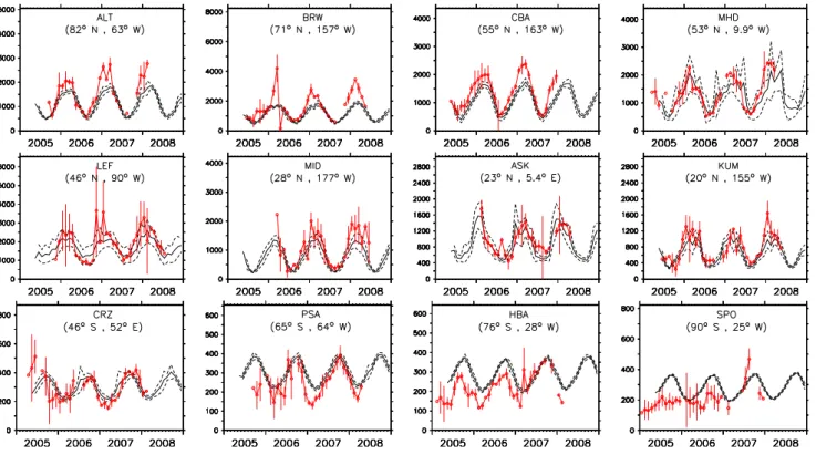
Fig. 2.Comparison of simulated and observed C2H6mixing ratios in pmol/mol for some selected locations (ordered by latitude). The red
lines and the bars represent the monthly averages and variability (calculated as the monthly standard deviations) of the measurements. The simulated monthly averages are indicated by the black lines and the corresponding simulated monthly variability (calculated as the monthly standard deviations of the simulated mixing ratios) by the dashed lines. The three letters at the center of each plot denote the station code (see http://www.esrl.noaa.gov/gmd/ccgg/flask.html). Note the different scales of the vertical axes.
weight. Values which are more representative for the aver-age conditions are weighted stronger, thus suppressing spe-cific episodes that cannot be expected to be reproduced by the model.
Generally, there is a much better agreement between the model simulations and the observations in the Northern Hemisphere (NH) extratropics than in the Southern Hemi-sphere (SH) extratropics, and the deviation from the obser-vations is largest in the tropics.
4.1 Ethane, C2H6
In Fig. 2 a comparison of the observations and the model simulation is shown for a number of locations. Notice that the seasonal cycle is correctly reproduced, although the model simulates a too low mixing ratio of ethane during the Northern Hemisphere (NH) winter (e.g., Alert, Canada, ALT, and Barrow, Alaska, BRW). On the other hand, the NH summer mixing ratios are reproduced correctly within the model/observation monthly variability (calculated as the monthly standard deviation of the observations). In the Southern Hemisphere (SH) the results are more difficult to interpret. Although the southern extratropics seem to be well simulated (see CRZ, Crozet Island, France), for polar sites (for example HBA, Halley Station, Antarctica) the model tends to simulate higher mixing ratios than observed. Fig. 3
Fig. 3. Seasonal cycle and latitudinal distribution of ethane (C2H6).
shows the latitudinal gradients and the seasonal cycle from observations and as calculated by the model. The model is able to reproduce the latitudinal mixing ratio changes, in-cluding the strong north-south gradient during all seasons.
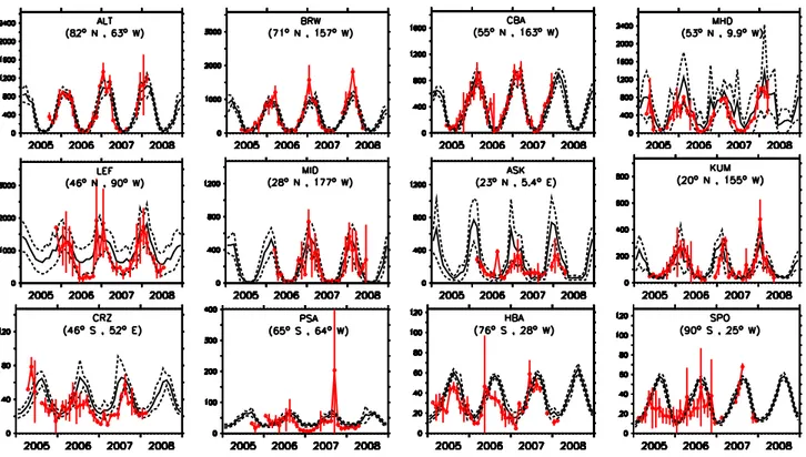
4.2 Propane, C3H8
As also shown in a previous analysis (Pozzer et al., 2007), the model simulation reproduces the main features observed for propane. The amplitude and phase of the simulated seasonal cycle also agree well with this new observational data set. As shown in Fig. 4, the seasonal cycle is well reproduced at the NH background sites (ALT and BRW). Moreover, Fig. 5 shows that not only the seasonal cycle is correctly re-produced, but also the latitudinal gradient. Generally, the model simulations agree well with the observations in the NH (where most of the emissions are located). However, at some locations (for example MHD, Mace Head, Ireland and LEF, Park Falls, USA) the model slightly overestimates the observed mixing ratios of propane. In addition, in the SH the simulated mixing ratios seem to be somewhat higher than the observations, especially during the SH winter (June, July and August) in remote regions, and during summer (January and February) in the SH extratropics. Clearly, these findings do not support a further increase of the emissions compared to the data used here.
4.3 n-butane, n-C4H10
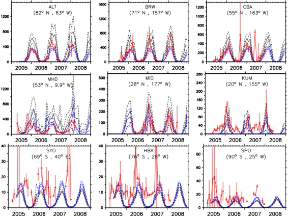
As mentioned in Sect. 4, E1 and E2 reproduce the observed phase of the seasonal cycle ofn-butane (Fig. 6 and Fig. 7). As observed by Blake et al. (2003) during the TOPSE cam-paign and also shown by the model, n-butane is removed quite rapidly at the onset of summer in all regions, and it is re-duced to low levels (almost depleted (single digit pmol/mol levels) by late spring, except at the highest latitudes. Exam-ples are (Fig. 7) ALT and BRW, where the simulated mix-ing ratios (both in simulation E1 and E2) decrease from ∼300–400 pmol/mol in April to ∼1–2 pmol/mol in June and remain at this level during the NH summer (July and August). The ability of the model to reproduce the observed seasonal cycle is also confirmed in Fig. 6, where a high cor-relation is found between the simulations and the observa-tions for staobserva-tions located between 40◦N and 90◦N. In
gen-eral, simulation E1 (based on anthropogenic emissions taken from the EDGAv2.0 database) produces higher mixing ra-tios at almost all locations in the NH compared to simulation E2, as shown in Fig. 6, where the normalised standard de-viations of model results from simulation E1 present values larger than 1. The opposite is the case in the SH, with lower mixing ratios in E1 than in E2. Simulation E1 seems to sys-tematically overestimate the winter maximum in the NH (see Fig. 7, ALT and CBA, Cold Bay, USA, and many others) while simulation E2 is closer to the observed mixing ratios.
Overall, for many stations, simulation E2 better represents the observed mixing ratios than E1 (see Fig. 6). Although a reasonable agreement of simulation E2 with the observa-tions is achieved at Midway Island (MID), and Cape Ku-mukahi (KUM), two typical marine boundary layer (MBL) background stations, the model underestimates the observed mixing ratios in the NH summer at these locations. This indicates that a nearby source ofn-butane may be present, hence that oceanic emissions potentially play a significant role. In the SH, both model simulations seem to underes-timaten-butane mixing ratios, with almost a total depletion during SH summer at remote locations, which is not observed in the flask data. While both model setups simulate values below 1 pmol/mol (∼0.5–0.6 pmol/mol) during SH summer (December, January and February), the observations indicate ∼10 pmol/mol. This difference suggests localizedn-butane emissions from the ocean. Additional high precision mea-surements of this tracer are needed to assess the role of the ocean in these remote areas.
4.4 i-butane, i-C4H10
4410 A. Pozzer et al.: Atmospheric C2-C5alkanes
Fig. 4.As Fig. 2 for C3H8.
Fig. 5. Seasonal cycle and latitudinal distribution of propane (C3H8). The colour code denotes the mixing ratios in pmol/mol,
calculated as a zonal average of the measurements available in the NOAA/ESRL GMD dataset. The superimposed contour lines de-note the zonal averages of the model results.
simulation E1. In contrast, at Wendower (UTA) simulation E1 is better than E2. For the SH, due to the low mixing ra-tios of i-butane (close to instrumental detection limit) and the high variability of the observations, it is difficult to draw a firm conclusion. However, at Halley Bay Station (HBA,
Antarctica) simulation E2 reproduces the first year of obser-vations (2005) better than E1.
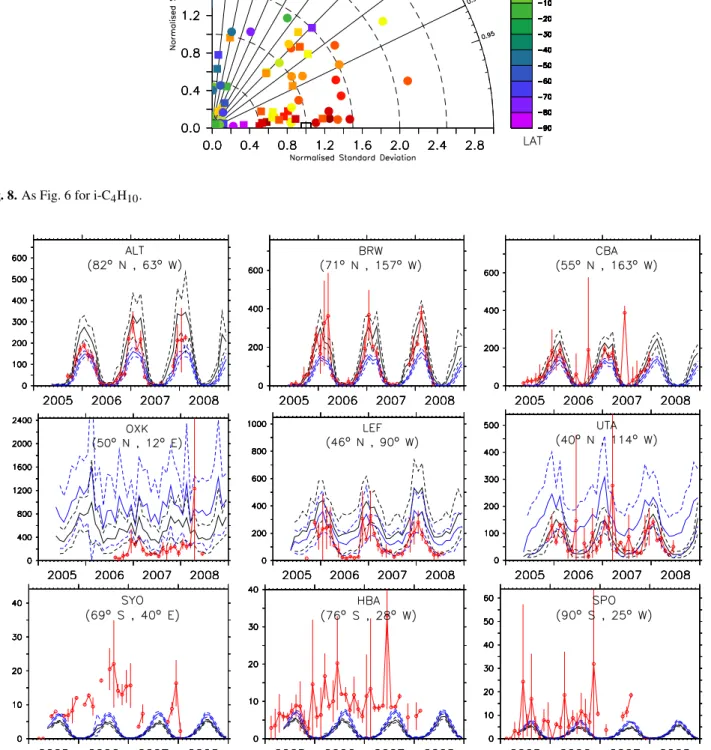
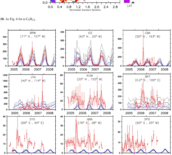
4.5 n-pentane, n-C5H12
As fori-butane, also for this tracer it is difficult to establish clearly which simulation better represents the observations, as both agree well with the observed values at the remote locations in the NH. The comparison between simulation re-sults and observations (Fig. 10) shows a poor agreement at stations located in the tropics and in the SH. In the NH, at lo-cations north of 60◦N, the centered pattern root mean square
(RMS) difference is similar for both simulations, whereas at locations between 20 and 30◦N simulation E1 is slightly
Fig. 6. Taylor diagram comparing monthly averages of n-C4H10from the model simulations with the surface observations from the NOAA
ESRL GMD network. The colour code denotes the geographic latitude. The symbol denote the model results: circle from simulation E1, square from simulation E2.
Fig. 7.Comparison of simulated and observed n-C4H10mixing ratios in pmol/mol for some selected locations (ordered by latitude). The
4412 A. Pozzer et al.: Atmospheric C2-C5alkanes
Fig. 8.As Fig. 6 for i-C4H10.
−
Fig. 10.As Fig. 6 for n-C5H12.
−
4414 A. Pozzer et al.: Atmospheric C2-C5alkanes underestimated in the SH. This is corroborated by similar
re-sults fori-pentane (see also Sect. 4.6). 4.6 i-pentane, i-C5H12
In contrast ton-pentane, north of 60◦N, the mixing ratios
from simulation E2 present a better agreement (i.e. lower centered pattern RMS difference) with the observations than simulation E1 (see Fig. 12). At these latitudes, the amplitude of the seasonal cycle is overestimated by at least 60% in sim-ulation E1 (visible from the normalised standard deviations), whereas it is within 40% in simulation E2. The overesti-mation of the simulated mixing ratios from simulation E1 with respect to the observations in the NH remote regions can be also seen in the time series plots (see Fig. 13, ALT), where it is highest during the NH winter, with a difference of a factor of 2. On the other hand, the model (both simu-lation E1 and E2) tends to underestimate the mixing ratios of i-C5H12in the NH subtropics and in the SH (see Fig. 13, MID and KUM). This systematic underestimation of the ob-served mixing ratios for the SH stations is again confirmed in Fig. 13. As mentioned in Sect. 4.5, this points to a partially wrong distribution of the emissions in the model, which are located almost exclusively in the NH, notably in the industri-alised regions.
4.7 Global C2-C5alkanes budgets
Following the analyses performed in Sects. 4.1–4.6, a global inventory of C2-C5 alkane emissions is shown in Table 2. Anthropogenic emissions are the most important sources in the budget of these tracers, ranging from∼75% (for ethane) to∼98% (for butanes and pentanes) of the total emissions. For butanes and pentanes, the dataset presented by Bey et al. (2001) (with an increased total emissions for pentanes) gives the best results with the EMAC model, and is recom-mended for future studies of these tracers. For ethane and propane, the model simulation with the EDGARv3.2 fast-track database gives satisfactory results.
Biomass burning is the second important source for ethane and propane, i.e.∼22% and ∼7% of the total sources, re-spectively. As shown by Helmig et al. (2008), biomass burn-ing effects on C3-C5alkanes is generally sporadic. Hence, the monthly average values of the observational dataset used here generally masked the biomass burning signal that could be observed. In addition the coarse model resolution and the low estimated value limit the possibilities to further evalu-ate this type of emission. These values could hence not be confirmed by our study and are reported as suggested in the literature.
Oceanic emissions play a small role in the budget for ethane and propane. The theoretical magnitude of oceanic emission for C4-C5is comparable to the one of biomass burn-ing, and hence too weak to be clearly distinguished in the ob-servational dataset. Nevertheless, our analysis suggests that
oceanic emissions can play a more significant role also for butanes and pentanes, at least at some coastal locations.
5 Contributions to the atmospheric budget of some OVOC
5.1 Acetone formation
Acetone (CH3COCH3), due to its photolysis, plays an im-portant role in the upper tropospheric HOx budget (Singh et al., 1995; McKeen et al., 1997; M¨uller and Brasseur, 1995; Wennberg et al., 1998; Jaegl´e et al., 2001) although re-cent studies have considerably reduced it (Blitz et al., 2004). Moreover, this trace gas is essential to correctly describe the ozone enhancement in flight corridors (Br¨uhl et al., 2000; Folkins and Chatfield, 2000). Oxidation of propane and C4-C5 isoalkanes (Singh et al., 1994) has been estimated to be ∼20–30% of the total sources of acetone (Jacob et al., 2002; Singh et al., 2004). It must be however stressed that there is still no agreement on the acetone budget. Recent studies, in fact, have modified significantly the estimated sources/sinks. Following recent studies, it is now widely thought that acetone has a net sink in the ocean (Singh et al. (2004), Marandino et al. (2005), and Taddei et al. (2009)). The lack of emissions from the ocean in the budget, however, is partially compensated by two other terms in the acetone budget:
– reduced photolysis, following the studies of Blitz et al. (2004) and Arnold et al. (2005).
– increased biogenic emissions. As pointed out by Singh et al. (2004, see also references therein), new measure-ments suggest higher biogenic emissions than the one proposed by Jacob et al. (2002) (33 Tg/yr). Based on the modeling study of Potter et al. (2003), the biogenic emissions should be in the range of 50–170 Tg/yr. The transport and chemical production of acetone were explicitly calculated with EMAC. Since E2 better repro-duces the observations, we used the results of this simula-tion to quantify the acetone producsimula-tion. Globally, the total production of acetone from C3-C5 alkanes is 21.3 Tg/yr in E2. The propane decomposition, with a yield of 0.73, pro-duces∼11.2 Tg/yr of acetone, which is higher than the to-tal production of acetone from C4-C5isoalkanes oxidation, namely 10.1 Tg/yr. In fact,i-butane oxidation produces 4.3 Tg/yr acetone, while 5.8 Tg/yr of acetone are produced by
i-pentane oxidation. This is the same for both simulations, because total emissions are equal. Despite the fact that both simulations produce very similar amounts of acetone, the production is distributed quite differently in the two simu-lations.
Fig. 12.As Fig. 6 for i-C5H12.
−
4416 A. Pozzer et al.: Atmospheric C2-C5alkanes
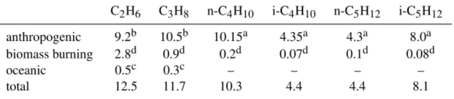
Table 2.Global source estimates of C2-C5alkanes based on the present EMAC simulations (in Tg(species)/yr).
C2H6 C3H8 n-C4H10 i-C4H10 n-C5H12 i-C5H12
anthropogenic 9.2b 10.5b 10.15a 4.35a 4.3a 8.0a biomass burning 2.8d 0.9d 0.2d 0.07d 0.1d 0.08d
oceanic 0.5c 0.3c – – – –
total 12.5 11.7 10.3 4.4 4.4 8.1
asimulation E2, with emissions distribution from Bey et al. (2001); bbased on EDGARv3.2, fast-track 2000;
cbased on Plass-D¨ulmer et al. (1995);
destimates based on Van der Werf et al. (2004) and Andreae and Merlet (2001) for the year 2000 (see Sect. 2.2.2).
Fig. 14. Difference between the simulated annual average surface mixing ratios of CH3COCH3from simulation E1 and the simula-tion E2, in nmol/mol (E1–E2).
E2. On the other hand, simulation E2 indicates a stronger production of acetone in the eastern USA, China, and in the SH. In both model simulations, CH3COCH3is produced al-most solely by the reaction of the iso-alkanes with OH; the contributions of the reactions with Cl and NO3are negligible, being less than 0.5% of the total. Our result partially con-firms the conclusion of Jacob et al. (2002), who calculated an acetone production of 14 Tg/yr, 4.0 Tg/yr and 2.6 Tg/yr from propane,i-butane andi-pentane, respectively. The dif-ferent acetone production compared to the study of Jacob et al. (2002) (present for propane andi-pentane decomposi-tion) arise from the different emissions and/or the acetone yield. For instance, Jacob et al. (2002) used an acetone yield of 0.53 fromi-pentane (from the reaction with OH). In our study an acetone yield of∼0.90 fromi-pentane was obtained. In addition the i-pentane emissions are substan-tially different, being 6.0 and 8.0 Tg/yr in the study of Jacob et al. (2002), and our study, respectively. For propane, the acetone yield is very similar (0.72) to the one obtained here (0.73), but a difference in the emissions (13.5 vs. 11.7 Tg/yr)
causes a slight difference in the acetone production. Because the E2 results reproduce i-butane and i-pentane better, we use this model simulation for the comparison with the eval-uation simulation S1 (see Sect. 2). The S1 analysis did not account for C4-C5alkanes and their subsequent atmospheric reactions. This allows us to evaluate the effect of higher alka-nes on acetone.
The resulting increase of the acetone mixing ratios is ev-ident, especially in the NH. As shown in Fig. 15, the ace-tone mixing ratio increased at the surface between 100 and 300 pmol/mol in NH remote areas, with the highest val-ues reached in locations downwind of polluted regions (for example over the Pacific and Atlantic Ocean). The rela-tive effect in polluted regions is smaller (maximum increase ∼30%) due to the strong anthropogenic emission of acetone. However, the contributions from the alkanes oxidation are significant (up to 1 nmol/mol). The strongest production re-gions are located over polluted rere-gions such as the eastern USA, the Mediterranean area and the China-Japan region. Here the maximum effect of C4-C5 alkanes on acetone is achieved, with an increase of∼1 nmol/mol. The mixing ra-tio of acetone in the SH is practically not affected by chem-ical formation from iso-alkanes, with the exception of a few locations in South America, simply because they are mainly emitted in the NH. This, combined with their short lifetime (shorter than the interhemispheric exchange time), confine the iso-alkanes to decompose and produce acetone only in the NH.
Fig. 15. Difference between the simulated annual average surface mixing ratios of CH3COCH3from simulation E2 and the evaluation simulation S1, in pmol/mol (E2–S1).
is∼50% compared to a simulation without C4-C5 alkanes. The simulated mixing ratios thus agree much better with the measurements. Especially below 5 km altitude, the sim-ulated vertical profiles are closer to the observations, and improved compared to simulation S1. In a polluted region (TRACE-P, Fig. 16) downwind of China, the inclusion of C4-C5 compounds results in a remarkable improvement of the acetone simulation. The underestimation of the free-troposphere mixing ratios seems to support the revision of the acetone quantum yield, as proposed by Blitz et al. (2004). Arnold et al. (2005), in fact, calculated an average increase of∼60–80% of acetone in the upper troposphere. It must be stressed, however, that in two cases the comparison between the model results from simulation E2 and field campaigns de-teriorates compared to the evaluation simulation S1. These are presented in Fig. 16 (bottom). Both cases are located in Japan, where the model, after the inclusion of C4-C5 oxida-tion pathways in the chemistry scheme, simulates mixing ra-tios that are higher than the observations. This could be due to a too strong source of C4-C5alkanes in the region in simu-lation E2, or alternatively, an overestimation/underestimation of direct acetone emissions/depositions.
5.2 Acetaldehyde formation
Acetaldehyde (CH3CHO) is also formed during the chem-ical degradation of C3-C5 alkanes. This tracer is a short-lived compound, with an average lifetime of several hours (Tyndall et al., 1995, 2002). It is an important precursor of PAN (peroxyacetyl nitrate), being a reservoir species of NOx (see Singh et al., 1985; Moxim et al., 1996). Oxidation of alkanes is responsible for ∼15–19% of the total acetalde-hyde emissions (Singh et al., 2004), or∼20–27% based on a more recent estimate (Millet et al., 2010). In this study, using the EMAC model, the calculated global production
−
Fig. 16. Vertical profiles of CH3COCH3(in pmol/mol) for some
4418 A. Pozzer et al.: Atmospheric C2-C5alkanes of acetaldehyde from C2-C5alkanes is 30.8 Tg/yr. In both
simulations E1 and E2, 18.1 Tg/yr and 3.1 Tg/yr of ac-etaldehyde are formed by the oxidation of ethane (C2H6) and propane (C3H8), respectively. In addition, 3.4 Tg/yr, 1.4 Tg/yr and 4.8 Tg/yr of acetaldehyde result from the ox-idation of n-butane (n-C4H10),n-pentane (n-C5H12) andi -pentane (i-C5H12), respectively. These amounts are almost exclusively produced by the reaction with OH; in fact, the reaction of C3-C5alkanes with NO3produces only 0.1% of the total acetaldehyde.
6 Conclusions
We compared the EMAC model results of C2-C5 alkanes with new observational data obtained from flask measure-ments from the NOAA/ESRL flask sampling network. Two emission distribution databases for butanes and pentanes (and associated isomers) were evaluated, new emissions of C2-C5estimated, and the effect of C3-C5alkanes on the con-centrations of acetone and acetaldehyde calculated.
Overall, the model reproduces the observations of ethane and propane mixing ratios well using the EDGARv3.2 emis-sion database (van Aardenne et al., 2005). The seasonal cy-cle is correctly reproduced, and the simulated mixing ratios are generally within 20% of the observations for ethane and propane. The simulation of ethane (C2H6) shows a good agreement with the observations, both with respect to the spatial and the temporal distribution, although with some un-derestimation in the NH during winter. In the SH a general overestimation is found, especially during the SH summer. Propane (C3H8) is reproduced well in the NH, while in the SH an overestimation occurs during the SH winter.
To compare two different emissions databases, two sen-sitivity simulations were performed. In simulation E1 the EDGARv2 (Olivier et al., 1999) emissions for butanes and pentanes, and in simulation E2 the emission distributions suggested by Bey et al. (2001) were used. Generally, the sim-ulated seasonal cycles of the butanes and pentanes agree well with the observations in both simulations. However, simu-lation E2 reproduces more realistically both, n-butane and
i-pentane, while fori-butane andn-pentane it is not evident which simulation is better, one being at the higher end of the observations (E1) and the other at the lower end (E2). In conclusion, we recommend the emission database suggested by Bey et al. (2001) (with additionally increased pentanes emissions) for future studies of these tracers. In addition, our analysis suggests a larger source from the ocean than what is currently assumed. A simulation with higher spatial resolu-tion would give addiresolu-tional informaresolu-tion on the global impact of biomass burning on these tracers, which, due to the small emitted amount compared to anthropogenic emissions, is dif-ficult to analyse and quantify with this low resolution model. The inclusion of C4-C5 alkanes in the model improves the representation of acetone (CH3COCH3). Based on
simulation E2,i-butane andi-pentane degradation produces ∼4.3 and∼5.8 Tg/yr of acetone, respectively. At the same time, the formation of acetaldehyde was also calculated, resulting in a production rate of 3.4 Tg/yr, 1.4 Tg/yr and 4.8 Tg/yr from the oxidation ofn-butane, n-pentane andi -pentane, respectively. The role of NO3and Cl radicals in the degradation of C3-C5isoalkanes and the formation of ace-tone and acetaldehyde is negligible, contributing less than 1% to the total chemical production.
Acknowledgements. We would like to thank Tzung-May Fu for providing the emissions used for simulation E2. We wish also to acknowledge the use of the Ferret program for analysis and graphics in this paper. Ferret is a product of NOAA’s Pacific Marine Environmental Laboratory (information is available at http://www.ferret.noaa.gov). We are grateful for the efforts of all NOAA sampling personnel, contributing to the dataset used in this study.
The service charges for this open access publication have been covered by the Max Planck Society.
Edited by: B. N. Duncan
References
Andreae, M. O. and Merlet, P.: Emission of trace gases and aerosols from biomass burning, Global Biogeochem. Cy., 15, 955–966, 2001.
Arnold, S. R., Chipperfield, M. P., and Blitz, M.: A three-dimensional model study of the effect of new temperature-dependent quantum yields for acetone photolysis, Geophys. Res. Lett., 110, D22305, doi:10.1029/2005JD005998, 2005. Atkinson, R.: Atmospheric chemistry of VOCs and NOx, Atmos.
Environ., 34, 2063–2101, 2000.
Bey, I., Jacob, D. J., Yantosca, R. M., Logan, J. A., Field, B. D., Fiore, A. M., Li, Q., Liu, H. Y., Mickley, L. J., and Schultz, M. G.: Global modeling of tropospheric chemistry with assim-ilated meteorology: Model description and evaluation, J. Geo-phys. Res., 106, 23073–23095, 2001.
Blake, D. and Rowland, S.: Urban leakage of liquefied petroleum gas and its impact on Mexico City air quality, Science, 269, 953– 956, 1995.
Blake Jr., D. R., T. S., T.-Y-Chen, Whipple, W., and Rowland, F. S.: Effects of biomassburning on summertime nonmethane hy-drocarbon concentrationsin the Canadian wetlands, J. Geophys. Res., 99, 1699–1719, 1993.
Blake, N., R., B. D., Sive, B., Ketzenstein, A. S., Meinardi, S., Win-genter, O., Atlas, E. L., Flocke, F., Ridley, B. A., and Sherwood, F.: The seasonalevolution of NMHCs and light alkyl nitrates at mniddle to high northern latitudes during TOPSE, J. Geophys. Res., 108, 8359, doi:10.1129/2001JD001467, 2003.
Bozzano, R., Siccardi, A., Schiano, M. E., Borghini, M., and Castel-lari, S.: Comparison of ECMWF surface meteorology and buoy observations in the Ligurian Sea, Ann. Geophys., 22, 317–330, doi:10.5194/angeo-22-317-2004, 2004.
Broadgate, W. J., Liss, P. S., and Penkett, S. A.: Seasonal emissions of isoprene and other reactive hydrocarbon gases from the ocean, Geophys. Res. Lett., 24, 2675–2678, 1997.
Br¨uhl, C., P¨oschl, U., Crutzen, P. J., and Steil, B.: Acetone and PAN in the upper troposphere: impact on ozone production from aircraft emissions, Atmos. Environ., 34, 3931–3938, 2000. Brunner, D., Staehelin, J., Rogers, H. L., K¨ohler, M. O., Pyle, J. A.,
Hauglustaine, D., Jourdain, L., Berntsen, T. K., Gauss, M., Isak-sen, I. S. A., Meijer, E., van Velthoven, P., Pitari, G., Mancini, E., Grewe, G., and Sausen, R.: An evaluation of the performance of chemistry transport models by comparison with research air-craft observations. Part 1: Concepts and overall model perfor-mance, Atmos. Chem. Phys., 3, 1609–1631, doi:10.5194/acp-3-1609-2003, 2003.
Cardelino, C. A. and Chameides, W. L.: Natural hydrocarbons, urbanization, and urban ozone, J. Geophys. Res., 95, 13971– 13979, 1990.
Daescu, D., Sandu, A., and Carmichael, G.: Direct and Adjoint Sensitivity Analysis of Chemical Kinetic Systems with KPP: II – Validation and Numerical Experiments, Atmos. Environ., 37, 5097–5114, 2003.
Damian, V., Sandu, A., Damian, M., Potra, F., and Carmichael, G.: The Kinetic PreProcessor KPP – A Software Environment for Solving Chemical Kinetics, Computers and Chemical Engineer-ing, 26, 2002.
Emmons, L. K., Hauglustaine, D. A., M¨uller, J.-F., Carroll, M. A., Brasseur, G. P., Brunner, D., Staehelin, J., Thouret, V., and Marenco, A.: Data composites of airborne observations of tropo-spheric ozone and its precursors, J. Geophys. Res., 105, 20497– 20538, 2000.
Etiope, G. and Ciccioli, P.: Earth’s Degassing: A Missing Ethane and Propane Source, Science, 323, p. 478, 2009.
Folberth, G. A., Hauglustaine, D. A., Lathi`ere, J., and Brocheton, F.: Interactive chemistry in the Laboratoire de Mtorologie Dy-namique general circulation model: model description and im-pact analysis of biogenic hydrocarbons on tropospheric chem-istry, Atmos. Chem. Phys., 6, 2273–2319, doi:10.5194/acp-6-2273-2006, 2006.
Folkins, I. and Chatfield, R.: Impact of acetone on ozone production and OH in the upper troposphere at high NOx, J. Geophys. Res., 105, 11585–11599, 2000.
Friedrich, R. and Obermeier, A.: Anthropogenic emissions of volatile organic compounds, Academic, San Diego, California, 2–38, 1999.
Gautrois, M., Brauers, T., Koppmann, R., Rohrer, F., Stein, O., and Rudolph, J.: Seasonal variability and trends of volatile organic compounds in the lower polar troposphere, J. Geophys. Res., 108, 4393, doi:10.1029/2002JD002765, 2003.
Goldan, P. D., Kuster, W., Fehsenfeld, F., and Montzka, S.: Hy-drocarbon measurements in the southeastern United States: The Rural Oxidants in the Southern Environment (ROSE) program 1990, J. Geophys. Res., 100, 35945–35963, 1995.
Goldan, P. D., Parrish, D. D., Kuster, W. C., Trainer, M., Mc-Keen, S., Holloway, J., Jobson, B., Sueper, D., and Fehsen-feld: Airborne measurements of isoprene,CO, and anthropogenic
hydrocarbons and their implications, J. Geophys. Res., 105, 9091–9105, 2000.
Guenther, A., Hewitt, C. N., Erickson, D., Fall, R., Geron, C., Graedel, T., Harley, P., Klinger, L., Lerdau, M., McKay, W. A., Pierce, T., Scholes, B., Steinbrecher, R., Tallamraju, R., Taylor, J., and Zimmerman, P.: A global model of natural volatile or-ganic compound emissions, J. Geophys. Res., 100, 8873–8892, 1995.
Guenther, A., Geron, C., Pierce, T., Lamb, B., Harley, P., and Fall, R.: Natural emissions of non-methane volatile organic com-pounds, carbon monoxide, and oxides of nitrogen from North America, Atmos. Environ., 34, 2205–2230, 2000.
Gupta, M. L., Cicerone, R. J., Blake, D. R., Rowland, F. S., and Isaksen, I. S. A.: Global atmospheric distributions and source strengths of light hydrocarbons and tetrachloroethene, J. Geo-phys. Res., 103, 28219–28235, 1998.
Haas-Laursen, D. and Hartley, D.: Consistent sampling methods for comparing models to CO2flask data, J. Geophys. Res., 102,
19059–19071, 1997.
Hagerman, L. M., Aneja, V. P., and Lonneman, W. A.: Characteriza-tion of non-methane hydrocarbons in the rural southeast United States, Atmos. Environ., 23, 4017–4038, 1997.
Helmig, D., Tanner, D., Honrath, R., Owen, R., and Parrish, D.: Nonmethane hydrocarbons at Pico Mountain, Azores: 1. Oxi-dation chemistry in the North Atlantic region, J. Geophys. Res., 113, D20S91, doi:10.1029/2007JD008930, 2008.
Houweling, S., Dentener, F., and Lelieveld, J.: The impact of non-methane hydrocarbon compounds on tropospheric photochem-istry, J. Geophys. Res., 103, 10673–10696, 1998.
Jacob, D., Field, B., Jin, E., Bey, I., Li, Q., Logan, J., and Yantosca, R.: Atmospheric budget of acetone, J. Geophys. Res., 107, 4100, doi:10.1029/2001JD000694, 2002.
Jaegl´e, L., Jacob, D. J., Brune, W. H., and Wennberg, P. O.: Chem-istry of HOxradicals in the upper troposphere, Atmos. Environ., 35, 469–489, 2001.
Jeuken, A., Siegmund, P., Heijboer, L., Feichter, J., and Bengtsson, L.: On the potential assimilating meteorological analyses in a global model for the purpose of model validation, J. Geophys. Res., 101, 16939–16950, 1996.
Jobson, B. T., Wu, Z., Niki, H., and Barrie, L. A.: Seasonal trends of isoprene, alkanes, and acetylene at a remote boreal site in Canada, J. Geophys. Res., 99, 1589–1599, 1994.
J¨ockel, P., Sander, R., Kerkweg, A., Tost, H., and Lelieveld, J.: Technical Note: The Modular Earth Submodel System (MESSy) – a new approach towards Earth System Modeling, Atmos. Chem. Phys., 5, 433–444, doi:10.5194/acp-5-433-2005, 2005. J¨ockel, P., Tost, H., Pozzer, A., Br¨uhl, C., Buchholz, J., Ganzeveld,
L., Hoor, P., Kerkweg, A., Lawrence, M. G., Sander, R., Steil, B., Stiller, G., Tanarhte, M., Taraborrelli, D., van Aardenne, J., and Lelieveld, J.: The atmospheric chemistry general circulation model ECHAM5/MESSy1: consistent simulation of ozone from the surface to the mesosphere, Atmos. Chem. Phys., 6, 5067– 5104, doi:10.5194/acp-6-5067-2006, 2006.
4420 A. Pozzer et al.: Atmospheric C2-C5alkanes
Kerkweg, A., Sander, R., Tost, H., and J¨ockel, P.: Technical note: Implementation of prescribed (OFFLEM), calculated (ON-LEM), and pseudo-emissions (TNUDGE) of chemical species in the Modular Earth Submodel System (MESSy), Atmos. Chem. Phys., 6, 3603–3609, doi:10.5194/acp-6-3603-2006, 2006b. Kerkweg, A., J¨ockel, P., Pozzer, A., Tost, H., Sander, R., Schulz,
M., Stier, P., Vignati, E., Wilson, J., and Lelieveld, J.: Consistent simulation of bromine chemistry from the marine boundary layer to the stratosphere – Part 1: Model description, sea salt aerosols and pH, Atmos. Chem. Phys., 8, 5899–5917, doi:10.5194/acp-8-5899-2008, 2008a.
Kerkweg, A., J¨ockel, P., Warwick, N., Gebhardt, S., Brenninkmei-jer, C. A. M., and Lelieveld, J.: Consistent simulation of bromine chemistry from the marine boundary layer to the stratosphere – Part 2: Bromocarbons, Atmos. Chem. Phys., 8, 5919–5939, doi:10.5194/acp-8-5919-2008, 2008b.
Kesselmeier, J. and Staudt, M.: Biogenic Volatile Organic Com-pounds (VOC): An Overview on Emission, Physiology and Ecol-ogy, J. Atmos. Chem., 33, 23–88, 1999.
Lee, H. B., Munger, J., Steven, C., and Goldstein, A. H.: Anthropogenic emissions of nonmethane hydrocarbons in the northeastern United Sates: Measured seasonal variations from 1992–1996 and 1999–2001, J. Geophys. Res., 111, D20307, doi:10.1029/2005JD006172, 2006.
Lelieveld, J., Br¨uhl, C., J¨ockel, P., Steil, B., Crutzen, P. J., Fis-cher, H., Giorgetta, M. A., Hoor, P., Lawrence, M. G., Sausen, R., and Tost, H.: Stratospheric dryness: model simulations and satellite observations, Atmos. Chem. Phys., 7, 1313–1332, doi:10.5194/acp-7-1313-2007, 2007.
Logan, J. A.: Tropospheric ozone: Seasonal behavior, trends, and anthropogenic influence, J. Geophys. Res., 90, 10463–10482, 1985.
Marandino, C., De Bruyn, W., Miller, S., Prather, M., and Saltzmann, E.: Oceanic uptake and the global atmo-spheric acetone budget, Geophys. Res. Lett., 32, L15806, doi:10.1029/2005GL023285, 2005.
McKeen, S. A., Gierczak, T., Burkholder, J. B., Wennberg, P. O., Hanisco, T. F., Keim, E. R., Gao, R.-S., Liu, S. C., Ravishankara, A. R., and Fahey, D. W.: The photochemistry of acetone in the upper troposphere: A source of odd-hydrogen radicals, Geophys. Res. Lett., 24, 3177–3180, 1997.
McLaren, R., Singleton, D. L., Lai, J. Y., Khouw, B., Singer, E., Wu, Z., and Niki, H.: Analysis of motor vehicle sources and their contribution to ambient hydrocarbon distributions at urban sites in Toronto during the Southern Ontario Oxidants Study, Atmos. Environ., 30, 2219–2232, 1996.
Middleton, P., Stockwell, W. R., and Carter, W. P. L.: Aggregation and analysis of volatile organic compound emissions for regional modeling, Atmos. Environ., 24A, 1107–1133, 1990.
Millet, D. B., Guenther, A., Siegel, D. A., Nelson, N. B., Singh, H. B., de Gouw, J. A., Warneke, C., Williams, J., Eerdekens, G., Sinha, V., Karl, T., Flocke, F., Apel, E., Riemer, D. D., Palmer, P. I., and Barkley, M.: Global atmospheric budget of acetaldehyde: 3-D model analysis and constraints from in-situ and satellite observations, Atmos. Chem. Phys., 10, 3405–3425, doi:10.5194/acp-10-3405-2010, 2010.
Moxim, W. J., Levy, H., and Kasibhatla, P. S.: Simulated global tropospheric PAN: Its transport and impact on NOx, J. Geophys.
Res., 101, 12621–12638, 1996.
M¨uller, J.-F. and Brasseur, G.: IMAGES: A three-dimensional chemical transport model of the global troposphere, J. Geophys. Res., 100, 16445–16490, 1995.
Neeb, P.: Structure-Reactivity Based Estimation of the Rate Con-stants for Hydroxyl Radical Reactions with Hydrocarbons, J. At-mos. Chem., 35, 295–315, 2000.
Olivier, J. G. J., Bouwman, A. F., van der Maas, C. W. M., Berdowski, J. J. M., Veldt, C., Bloos, J. P. J., Visschedijk, A. J. J., Zandveld, P. Y. J., and Haverlag, J. L.: Description of EDGAR Version 2.0: A set of global inventories of greenhouse gases and ozone-depleting substances for all anthrophogenic and most natural sources on a per country 1◦×1◦grid, RIVM Rep.
771060002, Rijksinstituut, Bilthoven, Netherlands, 1996. Olivier, J. G. J., Bloos, J. P. J., Berdowski, J. J. M., Visschedijk,
A. J. H., and Bouwman, A. F.: A 1990 global emission inven-tory of anthropogenic sources of carbon monoxide on 1◦×1◦
developed in the framework of EDGAR/GEIA, Chemosphere, 1, 1–17, 1999.
Parrish, D., Stohl, A., Forster, C., Atlas, E., Blake, D., Goldan, P., Kuster, W. C., and de Gouw, J.: Effects of mixing on evoultion of hydrocarbon ratios in the troposphere, J. Geophys. Res., 112, D10S34, doi:10.1029/2006JD007583, 2007.
Plass-D¨ulmer, C., Koppmann, R., Ratte, M., and Rudolph, J.: Light non-methane hydrocarbons in seawater, Global Biogeochem. Cy., 9, 79–100, 1995.
Poisson, N., Kanakidou, M., and Crutzen, P. J.: Impact of non-methane hydrocarbons on tropospheric chemistry and the oxidiz-ing power of the global troposphere: 3-dimensional modelloxidiz-ing results, J. Atmos. Chem., 36, 157–230, 2000.
Pollmann, J., Helmig, D., Hueber, J., Plass-D¨ulmer, C., and Tans, P.: Sampling,storage and analysisC2−C7non-methane
hydrocar-bons from the US National Oceanic and Atmospheric Adminis-tration Cooperative Air Sampling Network glass flasks, J. Chro-matogr. A, 1188, 75–87, 2008.
Potter, C., Klooster, S., Bubenheim, D., Singh, H. B., and Myneni, R.: Modeling terrestrial biogenic sources of oxygenated organic emissions, Earth Interaction, 7, 1–15, 2003.
Pozzer, A., J¨ockel, P., Tost, H., Sander, R., Ganzeveld, L., Kerk-weg, A., and Lelieveld, J.: Simulating organic species with the global atmospheric chemistry general circulation model ECHAM5/MESSy1: a comparison of model results with obser-vations, Atmos. Chem. Phys., 7, 2527–2550, doi:10.5194/acp-7-2527-2007, 2007.
Pozzer, A., J¨ockel, P., and Van Aardenne, J.: The influence of the vertical distribution of emissions on tropospheric chemistry, At-mos. Chem. Phys., 9, 9417–9432, doi:10.5194/acp-9-9417-2009, 2009.
Roberts, J., Jutte, R., Fehsenfeld, F., Albriton, D., and Sievers, R.: Measurements of anthropogenic hydrocarbon concentration ratios in the rural troposphere: Discrimination between back-ground and urban sources, Atmos. Environ., 19, 1945–1950, 1985.
Roeckner, E., Brokopf, R., Esch, M., Giorgetta, M., Hagemann, S., Kornblueh, L., Manzini, E., Schlese, U., and Schulzweida, U.: Sensitivity of simulated climate to horizontal and vertical resolution in the ECHAM5 atmosphere model, J. Climate, 19, 3771–3791, 2006.
hydrocarbon chemistry, J. Geophys. Res., 105, 22697–22712, 2000.
Rood, R. B.: Numerical advection algorithms and their role in at-mospheric transport and chemistry models, Rev. Geophys., 25, 71–100, 1987.
Rudolph, J.: The tropospheric distribution and budget of ethane, J. Geophys. Res., 100, 11369–11381, 1995.
Saito, T., Yokouchi, Y., and Kawamura, K.: Distribution of C2–C6 hydrocarbons over the western north Pacific and eastern Indian Ocean, Atmos. Environ., 34, 4373–4381, 2000.
Salstein, D., Ponte, R., and Cady-Pereira, K.: Uncertainties in atmo-spheric surface pressure fields from global analyses, J. Geophys. Res., 113, D14107, doi:10.1029/2007JD009531, 2008.
Sander, R., Kerkweg, A., J¨ockel, P., and Lelieveld, J.: Technical note: The new comprehensive atmospheric chemistry module MECCA, Atmos. Chem. Phys., 5, 445–450, doi:10.5194/acp-5-445-2005, 2005.
Sandu, A., Daescu, D., and Carmichael, G.: Direct and Adjoint Sensitivity Analysis of Chemical Kinetic Systems with KPP: I – Theory and Software Tools, Atmos. Environ., 37, 5083–5096, 2003.
Saunders, S. M., Jenkin, M. E., Derwent, R. G., and Pilling, M. J.: Protocol for the development of the Master Chemical Mech-anism, MCM v3 (Part A): tropospheric degradation of non-aromatic volatile organic compounds, Atmos. Chem. Phys., 3, 161–180, doi:10.5194/acp-3-161-2003, 2003.
Seinfeld, J. H. and Pandis, S.: Atmospheric Chemistry and Physics: From Air Pollution to Climate Change, Wiley-Interscience, 1997.
Sharma, U. K., Kajii, Y., and Akimoto, H.: Seasonal variation of C2-C6NMHCs at Happo, a remote site in Japan, Atmos.
Envi-ron., 34, 4447–4458, 2000.
Singh, H., Salas, l., Chatfield, R., Czech, E., Fried, A., Walega, J., Evans, M., Field, B., Jacob, D., Blake, D., Heikes, B., Talbot, R. andSachse, G., Crawford, J., Avery, M., Sandholm, S., and Fuelberg, H.: Analysis of the atmospheric distriburion, sources, and sinks of oxygenated volatile organic chemicals based in mea-surements over the Pacific during TRACE-P, J. Geophys. Res., 105(D3), D15S07, doi:10.1029/2003JD003883, 2004.
Singh, H. B. and Zimmermann, P.: Atmospheric distribution and sources of nonmethane hydrocarbons, John Wiley, New York, 1992.
Singh, H. B., O’Hara, D., Herlth, D., Sachse, W., Blake, D. R., Bradshaw, J. D., Kanakidou, M., and Crutzen, P. J.: Acetone in the atmosphere: Distribution, source, and sinks, J. Geophys. Res., 99, 1805–1819, 1994.
Singh, H. B., Kanakidou, M., Crutzen, P. J., and Jacob, D. J.: High concentrations and photochemical fate of oxygenated hydrocar-bons in the global troposphere, Nature, 378, 50–54, 1995. Singh, H. B., Chen, Y., Staudt, A. C., Jacob, D. J., Blake, D. R.,
Heikes, B. G., and Snow, J.: Evidence from the Pacific tro-posphere for large global sources of oxygenated organic com-pounds, Nature, 410, 1078–1081, 2001.
Singh, H. B., Tabazadeh, A., Evans, M. J., Field, B. D., Jacob, D. J., Sachse, G., Crawford, J. H., Shetter, R., and Brune, W. H.: Oxygenated volatile organic chemicals in the oceans: Inferences and implications based on atmospheric observations and air-sea exchange models, Geophys. Res. Lett., 30, 1862, doi:10.1029/2003GL017933, 2003.
Singh, H. B., Salas, L. J., Ridley, B. A., Shetter, J. D., Donahue, N. M., Fehsenfeld, F. C., Fahey, D. W., Parrish, D. D., Williams, E. J., Liu, S. C., H¨ubler, G., and Murphy, P. C.: Relationship between peroxyacetyl nitrate (PAN) and nitrogen oxides in the clean troposphere, Nature, 318, 347–349, 1985.
Spivakovsky, C. M., Logan, J. A., Montzka, S. A., Balkanski, Y. J., Foreman-Fowler, M., Jones, D. B. A., Horowitz, L. W., Fusco, A. C., Brenninkmeijer, C. A. M., Prather, M. J., Wofsy, S. C., and McElroy, M. B.: Three-dimensional climatological distribution of tropospheric OH: Update and evaluation, J. Geophys. Res., 105, 8931–8980, 2000.
Swanson, A., Blake, N., Atlas, E., Flocke, F., Blake, D. R., and Sherwood, F.: Seasonal variation ofC2−C4 nonmethane
hydrocarbons and C1−C4 alkyl nitrates at the Summit re-search station in Greenland, J. Geophys. Res., 108, 4065, doi:10.1129/2001JD001445, 2003.
Taddei, S., Toscano, P., Gioli, B., Matese, A., Miglietta, F., Vaccari, F. P., Zaldei, A., Custer, T., and Williams, J.: Carbon Dioxide and Acetone AirSea Fluxes over the Southern Atlantic, Environ. Sci. Technol., 43, 5218–5222, 2009.
Taylor, K.: Summarizing multiple aspects of model performance in a single diagram, J. Geophys. Res., 106, 7183–7192, 2001. Tost, H., J¨ockel, P., Kerkweg, A., Sander, R., and Lelieveld, J.:
Technical note: A new comprehensive SCAVenging submodel for global atmospheric chemistry modelling, Atmos. Chem. Phys., 6, 565–574, doi:10.5194/acp-6-565-2006, 2006.
Tyndall, G. S., Staffelbach, T. A., Orlando, J. J., and Calvert, J. G.: Rate coefficients for the reactions of OH radicals with methyl-glyoxal and acetaldehyde, Int. J. Chem. Kinetics, 27, 1009–1020, 1995.
Tyndall, G. S., Orlando, J. J., Wallington, T. J., Hurley, M. D., Goto, M., and Kawasaki, M.: Mechanism of the reaction of OH radicals with acetone and acetaldehyde at 251 and 296 K, Phys. Chem. Chem. Phys., 4, 2189–2193, 2002.
van Aardenne, J., Dentener, F., Olivier, J., Peters, J., and Ganzeveld, L.: The EDGAR 3.2 Fast Track 2000 dataset (32FT2000), online available at: http://www.mnp.nl/edgar/model/v32ft2000edgar/ docv32ft2000/, 2005.
van Aardenne, J. A., Dentener, F. J., Olivier, J. G. J., Klein Gold-ewijk, C. G. M., and Lelieveld, J.: A 1deg×1deg resolution data set of historical anthropogenic trace gas emissions for the period 1890–1990, Global Biogeochem. Cy., 15, 909–928, 2001. Van der Werf, G. R., Randerson, J. T., Collatz, G. J., Giglio, L.,
Kasibhatla, P. S., Avelino, A., Olsen, S. C., and Kasischke, E.: Continental-scale partitioning of fire emissions during the 1997– 2001 El Nino/La Nina period, Science, 303, 73–76, 2004. von Kuhlmann, R., Lawrence, M. G., Crutzen, P. J., and Rasch,
P. J.: A model for studies of tropospheric ozone and nonmethane hydrocarbons: Model description and ozone results, J. Geophys. Res., 108, 4294, doi:10.1029/2002JD002893, 2003a.
von Kuhlmann, R., Lawrence, M. G., Crutzen, P. J., and Rasch, P. J.: A Model for Studies of Tropospheric Ozone and Non-Methane Hydrocarbons: Model Evaluation of Ozone Related Species, J. Geophys. Res., 108, 4729, doi:10.1029/2002JD003348, 2003b. Wang, Y., Jacob, D. J., and Logan, J. A.: Global simulation of
4422 A. Pozzer et al.: Atmospheric C2-C5alkanes
Wennberg, P. O., Hanisco, T. F., Jaegl´e, L., Jacob, D., Hintsa, E. J., Lanzendorf, E. J., Anderson, J. G., Gao, R.-S., Keim, E. R., Don-nelly, S. G., Negro, L. A. D., Fahey, D. W., McKeen, S. A., Salawitch, R. J., Webster, C. R., May, R. D., Herman, R. L., Proffitt, M. H., Margitan, J. J., Atlas, E. L., Schauffler, S. M., Flocke, F., McElroy, C. T., and Bui, T. P.: Hydrogen radicals, nitrogen radicals, and the production of O3in the upper
tropo-sphere, Science, 279, 49–53, 1998.