The CU mobile Solar Occultation Flux instrument: structure
functions and emission rates of NH
3
, NO
2
and C
2
H
6
Natalie Kille1,2, Sunil Baidar2,3,a, Philip Handley2,3,a, Ivan Ortega2,3,b, Roman Sinreich3, Owen R. Cooper4, Frank Hase5, James W. Hannigan6, Gabriele Pfister6, and Rainer Volkamer1,2,3
1Department of Atmospheric and Oceanic Sciences (ATOC), University of Colorado, Boulder, CO, USA
2Cooperative Institute for Research in Environmental Sciences (CIRES), University of Colorado, Boulder, CO, USA 3Department of Chemistry and Biochemistry, University of Colorado, Boulder, CO, USA
4National Ocean Atmosphere Administration (NOAA), Chemical Sciences Division (CSD), Boulder, CO, USA 5Institut für Meteorologie und Klimaforschung – Atmosphärische Spurengase und Fernerkundung (IMK-ASF),
Karlsruhe Institute of Technology (KIT), Karlsruhe, Germany
6National Center for Atmospheric Research (NCAR), Atmospheric Chemistry Observations & Modeling Laboratory
(ACOM), Boulder, CO, USA
anow at: NOAA/CSD, Boulder, CO, USA bnow at: NCAR/ACOM, Boulder, CO, USA
Correspondence to:R. Volkamer ([email protected])
Received: 8 June 2016 – Published in Atmos. Meas. Tech. Discuss.: 24 August 2016 Revised: 25 December 2016 – Accepted: 7 January 2017 – Published: 1 February 2017
Abstract. We describe the University of Colorado mobile Solar Occultation Flux instrument (CU mobile SOF). The instrument consists of a digital mobile solar tracker that is coupled to a Fourier transform spectrometer (FTS) of 0.5 cm−1resolution and a UV–visible spectrometer (UV–vis)
of 0.55 nm resolution. The instrument is used to simulta-neously measure the absorption of ammonia (NH3), ethane
(C2H6) and nitrogen dioxide (NO2)along the direct solar
beam from a moving laboratory. These direct-sun observa-tions provide high photon flux and enable measurements of vertical column densities (VCDs) with geometric air mass factors, high temporal resolution of 2 s and spatial resolu-tion of 5–19 m. It is shown that the instrument line shape (ILS) of the FTS is independent of the azimuth and ele-vation angle pointing of the solar tracker. Further, collo-cated measurements next to a high-resolution FTS at the Na-tional Center for Atmospheric Research (HR-NCAR-FTS) show that the CU mobile SOF measurements of NH3 and
C2H6are precise and accurate; the VCD error at high
sig-nal to noise ratio is 2–7 %. During the Front Range Air Pollution and Photochemistry Experiment (FRAPPE) from 21 July to 3 September 2014 in Colorado, the CU mo-bile SOF instrument measured median (minimum,
maxi-mum) VCDs of 4.3 (0.5, 45)×1016molecules cm−2 NH3,
0.30 (0.06, 2.23)×1016molecules cm−2NO
2and 3.5 (1.5,
7.7)×1016molecules cm−2 C
2H6. All gases were detected
in larger 95 % of the spectra recorded in urban, semi-polluted rural and remote rural areas of the Colorado Front Range. We calculate structure functions based on VCDs, which de-scribe the variability of a gas column over distance, and find the largest variability for NH3. The structure functions
sug-gest that currently available satellites resolve about 10 % of the observed NH3 and NO2 VCD variability in the study
area. We further quantify the trace gas emission fluxes of NH3 and C2H6and production rates of NO2 from
concen-trated animal feeding operations (CAFO) using the mass balance method, i.e., the closed-loop vector integral of the VCD times wind speed along the drive track. Excellent re-producibility is found for NH3fluxes and also, to a lesser
ex-tent, NO2production rates on 2 consecutive days; for C2H6
the fluxes are affected by variable upwind conditions. Av-erage emission factors were 12.0 and 11.4 gNH3h−1head−1
at 30◦C for feedlots with a combined capacity for∼54 000 cattle and a dairy farm of ∼7400 cattle; the pooled rate of 11.8±2.0 gNH3h−1head−1 is compatible with the
source from cattle in Weld County, CO (535 766 cattle), could be underestimated by a factor of 2–10. CAFO soils are found to be a significant source of NOx. The NOxsource
ac-counts for∼1.2 % of the N flux in NH3and has the potential
to add∼10 % to the overall NOxemissions in Weld County
and double the NOx source in remote areas. This potential
of CAFO to influence ambient NOx concentrations on the
regional scale is relevant because O3formation is NOx
sen-sitive in the Colorado Front Range. Emissions of NH3and
NOx are relevant for the photochemical O3 and secondary
aerosol formation.
1 Introduction
Gases emitted from anthropogenic sources can have a pro-found impact on local air quality (Raga et al., 2001; Ra-manathan and Feng, 2009) and climate (IPCC, 2013). Emis-sions from large cattle feedlots contain ammonia (NH3;
Hutchinson et al., 1982; Flesch et al., 2007), which is a precursor for aerosol via the formation of ammonium salts (Walker et al., 2004). NH3is a major source for reactive
ni-trogen to form particulate matter 2.5 (PM2.5), which
nega-tively affects human health (Todd et al., 2008). Ammonium salts form when NH3 reacts with inorganic (Doyle et al.,
1979) and organic (Zhang et al., 2004) acids (Fangmeier et al., 1994). Ammonium is mainly present in the submicron fraction of aerosol and contributes significantly to PM2.5 mass worldwide (Zhang et al., 2007). Aerosol can travel a long distance in the atmosphere before deposition, thus af-fecting greater regions than the local environment (Hristov et al., 2011). Oil and natural gas (ONG) production is a source for fugitive emissions of ethane (C2H6; Xiao et al., 2008),
a small volatile alkane, and volatile organic carbon (VOC) precursor of ozone (O3; Parrish and Fehsenfeld, 2000). The
emissions of C2H6 from the ONG sector in areas of
hy-draulic fracturing are highly uncertain and are an area of ac-tive research with interest in emission rates, air quality and climate impacts (Ahmadov et al., 2015). C2H6 contributes
to oxidation production of formaldehyde (HCHO) and ac-etaldehyde (CH3CHO; Lou et al., 2007), which is a
car-cinogen and precursor for radicals that lead to photochem-ical O3 production (Lei et al., 2009; Baidar et al., 2013).
HCHO as a radical source also affects the oxidative capac-ity that is relevant for secondary aerosol formation (Fried et al., 1997; Franco et al., 2015). Nitrogen dioxide (NO2),
emitted during combustion, is a precursor for the formation of photochemical O3(Finlayson-Pitts and Pitts, 2000). Only
∼10 % of NOx (=NO+NO2)emissions from vehicles is
in the form of NO2 directly (Carslaw and Beevers, 2005).
Another source of NOx are soils from feedlots (Denmead
et al., 2008). Based on SCIAMACHY (Scanning Imaging Spectrometer for Atmospheric Chartography) satellite ob-servations, Australia and the Sahara produce NOx
predom-inantly from soil, whereas the United States predompredom-inantly produces NOxfrom anthropogenic sources, such as
combus-tion (Jaeglé et al., 2005; Bertram et al., 2005). Health effects of O3 and aerosols require assessment of emissions of the
precursor gases. The US Environmental Protection Agency (EPA) recently updated its guidelines for fenceline moni-toring to better protect communities near refineries (Jones, 2015).
The Solar Occultation Flux (SOF) method uses direct sunlight to determine vertically integrated concentrations of trace gases (Mellqvist et al., 2010; EPA Handbook, 2011; Jo-hansson et al., 2014b; Kim et al., 2011; European Commis-sion, 2015). The SOF method has been used on mobile plat-forms to measure ethene (de Gouw et al., 2009; Mellqvist et al., 2010; Johansson et al., 2014a, b), propane (Mellqvist et al., 2010; Johansson et al., 2014a, b) and alkanes including C2H6(Johansson et al., 2014b), C2H4and C3H6(Kim et al.,
2011). De Foy et al. (2007) used the SOF method station-ary to measure alkanes and NH3, amongst others. However,
no reports of NH3currently exist using the SOF method on
a mobile laboratory. Column observations integrate over the planetary boundary layer height (PBLH) and hence are inde-pendent of its changing height. Column measurements can be used to quantify the emission flux/production rate from an area source by driving around the source or driving up-wind and downup-wind of that source area. The SOF method is complementary to other techniques used to quantify emis-sions, such as in situ measurements, or stationary deploy-ment of several commercial EM27/SUN Fourier transform spectrometer (FTS) around an area source (Hase et al., 2015; Chen et al., 2016). In situ measurements, or open-path eddy covariance studies (Baum et al., 2008), provide more local-ized information and require access to the site of interest. Micrometeorological gradient methods require assumptions of homogeneity (Todd et al., 2008). One benefit of mobile SOF measurements is that the total amount is quantified re-motely, and no assumptions about homogeneity need to be made. With the mobile SOF a source can be isolated and quantified remotely. The emission flux and source strength is determined by the mass balance approach (Ibrahim et al., 2010; Mellqvist et al., 2010; Baidar et al., 2013).
Structure functions (Follette-Cook et al., 2015) character-ize how the variability in vertical column densities (VCDs) changes over distance (see Sects. 2.6 and 3.5). We use the structure function to characterize the VCD variability of NH3, NO2and C2H6on the spatial scale of a satellite ground
pixel. Satellites used to retrieve these gases are, for exam-ple, the Tropospheric Emission Spectrometer (TES) with a ground pixel size of 5.3×8.5 km2 and Infrared Atmo-spheric Sounding Interferometer (IASI) with a footprint of 12×25 km2for NH3(Shephard et al., 2011; Van Damme et
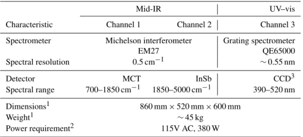
Detector MCT InSb CCD3 Spectral range 700–1850 cm−1 1850–5000 cm−1 390–520 nm
Dimensions1 860 mm×520 mm×600 mm
Weight1 ∼45 kg
Power requirement2 115V AC, 380 W
1Includes the solar tracker, spectrometers and base plate.2Includes the solar tracker, spectrometers, laptops for
data acquisition and control electronics.3Charge-coupled device.
Figure 1. (a)Conceptual sketch of the mobile SOF instrument com-ponents.(b)Picture of the instrument installed inside the trailer.
Coheur et al., 2007; Fischer et al., 2008; Glatthor et al., 2009; Höpfner et al., 2016), SCIAMACHY with a ground pixel size of 15×26 km2and Ozone Monitoring Instrument (OMI) with a resolution of 13×24 km2for NO2(Boersma et
al., 2009). With their large spatial coverage and continuous global monitoring, satellites have the potential to increase knowledge about the large distribution and cycles of gases. However, satellite observations remain not very well vali-dated (Dammers et al., 2016) and satellites quantifying C2H6
VCDs are not sensitive to the lower troposphere (Streets et al., 2013). Previous satellite comparisons have used mobile in situ measurements of NH3to characterize the near-surface
NH3mixing ratio variability in the San Joaquin Valley in
Cal-ifornia and compare with data from TES (Sun et al., 2015a) and CrIS (Cross-track Infrared Sounder) satellites (Shephard and Cady-Pereira, 2015). To our knowledge there currently is no attempt to characterize the sub-satellite ground pixel vari-ability using mobile VCD observations of NH3 and C2H6.
Mobile VCD measurements eliminate the need for assump-tions about NH3and C2H6vertical distributions.
2 Experimental design
instru-mentation was mounted inside a trailer with the solar tracker placed through the roof of the trailer.
2.1 Digital mobile solar tracker
The digital mobile solar tracker has been described in detail elsewhere (Baidar et al., 2016). In brief, it consists of a set of planar aluminum mirrors; one mirror is mounted directly on the axis of a stepper motor regulating the elevation angle and one is on a rotation stage regulating the azimuth angle. The mirrors are controlled from an embedded computer system (PC104) that is integrated with a motion compensation sys-tem to calculate the Euler angles of the sun for coarse track-ing and a real-time imagtrack-ing feedback loop for fine tracktrack-ing. During mobile deployment the solar tracker has a demon-strated angular precision of 0.052◦ and allows the reliable tracking of the sun even on uneven dirt roads from a mov-ing mobile laboratory. This trackmov-ing precision and first trace gas measurements have been demonstrated using the center to limb darkening (CLD) of solar Fraunhofer lines and NO2
lines at UV–vis wavelengths. The direct-sun differential op-tical absorption spectroscopy (DS-DOAS) NO2VCDs have
further been compared to NO2 VCDs measured by
MAX-DOAS (multi-axis MAX-DOAS; Baidar et al., 2016). Here, we describe the addition of an FTS to simultaneously measure trace gases at mid-IR wavelengths.
2.2 Mobile SOF EM27 FTS
A customized Bruker EM27 FTS was characterized for the use from mobile platforms coupled to the solar tracker, see Fig. 1. The EM27 FTS is a Michelson interferometer with a double pendulum corner cube mirror design. The oscillat-ing mirrors determine the optical path difference (OPD). Our configuration allows for fast scanning at 160 kHz to provide spectra acquisition with 2 Hz time resolution and includes a zinc selenide (ZnSe) beam splitter and window, 24 V power supply and a Stirling-cooled sandwich detector operating at 77 K, consisting of a mercury cadmium telluride (MCT) and an indium antimonide (InSb) detector in a single detector housing. Each detector has an active area of 1 nm diameter. The FTS allows for measurements over a wide spectral range in the mid-IR spectral region of the solar spectrum from 700 to 5000 cm−1. We did not use an apodization function for the measurements during FRAPPE. Boxcar was selected in order to keep the resolution at its maximum of 0.5 cm−1.
Further specifications about the instrument configuration are provided in Table 1.
The instrument characterization is described in Sect. 2.4.
2.2.1 NH3and C2H6retrieval
The spectra taken with the MCT detector were corrected for instrument background. An example solar spectrum mea-sured by the MCT and InSb detectors is shown in Fig. 2, where the micro windows used for the C2H6 and NH3
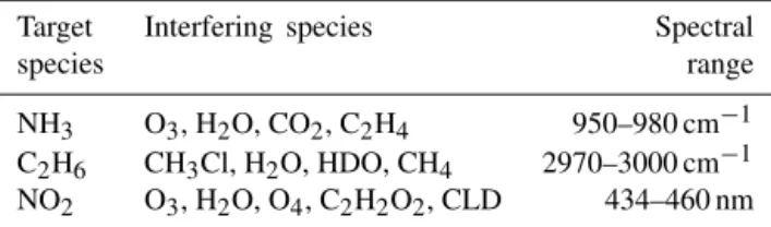
re-Table 2.Spectral fit windows used in the retrievals.
Target Interfering species Spectral
species range
NH3 O3, H2O, CO2, C2H4 950–980 cm−1 C2H6 CH3Cl, H2O, HDO, CH4 2970–3000 cm−1 NO2 O3, H2O, O4, C2H2O2, CLD 434–460 nm
trieval are highlighted with yellow bars. NH3 VCDs were
retrieved from MCT spectra using the micro window 950– 980 cm−1. The InSb spectra were used without further cor-rections for the retrieval of C2H6at 2970–3000 cm−1. The
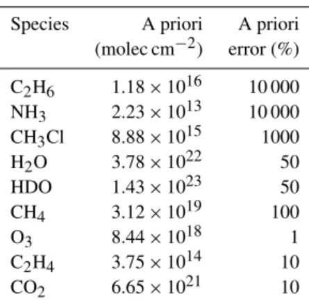
spectral fit windows including interfering species are listed in Table 2. All retrievals were conducted using the SFIT4 soft-ware (Hase et al., 2004; Nussbaumer and Hannigan, 2014) and a priori profile parameters as given in Table 3. SFIT4 uses the vertical profiles of pressure, temperature and wa-ter vapor taken from NCEP (National Cenwa-ters for Environ-mental Prediction) and WACCM (Whole Atmosphere Com-munity Climate Model, https://www2.acom.ucar.edu/gcm/ waccm) at given altitudes that were assumed to be constant throughout each day. It uses updated C2H6lines from
Harri-son et al. (2010) and HITRAN 2008 (Rothman et al., 2009) line lists for all other absorbers listed in Table 2. The a pri-ori error allows for the VCD of interest (NH3or C2H6)to
vary by a factor of 100 around the a priori value; the interfer-ing gases, e.g., CO2and H2O, were allowed less variability.
SFIT iterates to obtain a best fit between the calculated and measured spectrum. The residual parameter (%rms) is used to quality assure our data. The quality assurance cutoff %rms value has been determined by contrasting√1
N·noise against
the residual, whereN is the cumulative number of spectra that have a %rms less than or equal to the threshold, and noise is the spread of residuals within the threshold. The cutoff %rms has been taken as 3 times the minimum of the
1
√
N·noise against the residual plot and was determined to
be 3.6 for NH3and 6.4 for C2H6. This translates to∼75 %
of NH3and∼47 % of C2H6spectra being considered
dur-ing analysis. Spectral proof of the detection of both gases is shown in Fig. 2. In that shown case the detected gas column density of C2H6has a value of 7.13×10¹⁶molecules cm−2
and for NH3a value of 40.2×10¹⁶molecules cm−2, which is
well above the detection limit (see Sect. 3.1.1). The top panel of the fit window shows the residual between observed and fitted spectrum. Besides the observed and fitted spectrum the fit window also includes the strongest interfering trace gases.
2.3 UV–vis spectrometer
The UV–vis channel consists of an OceanOptics QE65000 grating spectrometer to measure NO2VCDs. The
spec-Figure 2. Solar spectrum measured by the InSb (blue) and MCT (green) detectors. Yellow bars indicate the spectral intervals used for the retrieval of C2H6 and NH3. Spectral proof of C2H6is shown on the top left and of NH3 on the top right. The C2H6column was 7.13×10¹⁶molecules cm−2(%rms=2.7) and the NH3column was 40.2×10¹⁶molecules cm−2(%rms=1.9) for the retrievals shown.
Table 3.Overview of SFIT4 a priori values.
Species A priori A priori (molec cm−2) error (%)
C2H6 1.18×10¹⁶ 10 000 NH3 2.23×10¹³ 10 000 CH3Cl 8.88×10¹⁵ 1000
H2O 3.78×10²² 50
HDO 1.43×10²³ 50
CH4 3.12×10¹⁹ 100
O3 8.44×10¹⁸ 1
C2H4 3.75×10¹⁴ 10
CO2 6.65×10²¹ 10
tral range 390–520 nm as is described elsewhere (Baidar et al., 2016).
2.3.1 NO2retrieval
NO2was measured by the UV–vis spectrometer using the
re-trievals described in Baidar et al. (2016). In brief, NO2was
retrieved in the spectral fitting window 434–460 nm using the WinDOAS software (Van Roozendael and Fayt, 2001). Baidar et al. (2016) also have compared the DS-DOAS NO2
VCDs with MAX-DOAS to assess benefits of high photon fluxes for sensitivity and validate the NO2measurements.
2.4 Mobile SOF characterization
2.4.1 Comparison at NCAR
Prior to field deployment, collocated measurements were performed with the mobile laboratory at the National Cen-ter for Atmospheric Research (NCAR) in Boulder, CO, with a high-resolution Bruker 120HR FTS (HR-NCAR-FTS). The CU mobile SOF instrument was mounted in a trailer that was parked in the parking lot∼50 m away from the HR-NCAR-FTS, assuring that both instruments observed the nearly same air mass. Coincident time intervals of the measurements were evaluated to determine the accuracy of the trace gas VCDs and the limit of detection (LOD) of the 0.5 cm−1resolution FTS. We calculate the LOD using the following IUPAC def-inition (IUPAC, 2006):
LODexp=k·σGaussian+ |background|, (1)
wherek is a factor chosen according to the confidence in-terval, andσGaussianis the standard deviation during a time
period in which the air mass is not changing (i.e., constant C2H6and NH3VCD). We setk=3 for a 99.7 % confidence
Table 4.Results of the FTS quality assurance.
Channel 1 Channel 2 /NH3 /C2H6
Precision1(1016molec cm−2) 0.01 0.01 Accuracy2(1016molec cm−2) 0.07 0.10 LOD (1016molec cm−2) 0.10 0.13
Total error (%) 4.4 6.7
OPD effect3(%) (2σ) 1.0 0.0
Cross section uncertainty (%) 2.04 4.05
Fit uncertainty (%) (2σ) 3.8 5.4
1Calculated as the mean during periods in which the atmosphere remained
constant.2Calculated as the difference between the CU mobile lab FTS and the NCAR high-resolution FTS.3Calculated for a median VCD of 4.32×10¹⁶molec cm−2for NH
3and 3.49×10¹⁶molec cm−2for C 2H6as
measured during RD10 and RD11.4Source: Kleiner et al. (2003).5Source: Harrison et al. (2010).
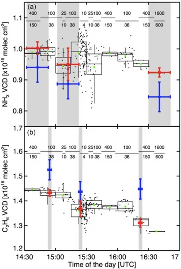
taken in a parking lot at CU (40.005◦N, 105.270◦W) to de-termineσGaussian, and they were found to be consistent with
theσGaussiandetermined at NCAR shown in Fig. 3. The
fig-ure shows the VCD measfig-urements of NH3 and C2H6 from
the HR-NCAR-FTS in blue and mobile SOF data in black. Mobile SOF VCD measurements were taken at specific inte-gration times. A longer inteinte-gration time averages more scans and reduces the noise in the data. For the background deter-mination mobile SOF data points within the integration time of one HR-NCAR-FTS were averaged. The background was calculated as the difference between mobile SOF FTS and HR-NCAR-FTS data points. See Sect. 3.1.1 for discussion on the comparison.
2.4.2 Characterization of the ILS
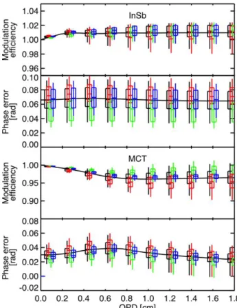
For measurements from the mobile laboratory the azimuth and elevation angles change rapidly over the course of an RD. It is therefore important to characterize the ILS (Hase et al., 1999) over a wide range of azimuth and elevation angle pairs. This was tested in a laboratory setup where the solar tracker was pointed at a globar to observe atmospheric water vapor over a distance of several meters along the path between the FTS and the globar. The light emitted by the globar is col-limated and directed onto the solar tracker. The FTS with solar tracker is positioned on a rotatable platform. The ILS has been determined using the retrieval code LINEFIT (Hase et al., 1999) version 14 using water vapor absorption lines in the spectral range at 1950–1900 for the InSb and at 1820– 1800 cm−1for the MCT detector. The modulation efficiency at maximum OPD is shown in Fig. 4 for different azimuthal and elevation angles, and the results are further discussed in Sect. 3.1.2 and Table 4.
Figure 3.Assessment of CU mobile SOF accuracy at NCAR, Boul-der, CO:(a)NH3and(b)C2H6. Blue: measurements of the HR-NCAR-FTS; black: individual mobile SOF measurements (variable integration time); red: mobile SOF data averaged over the time pe-riod of the NCAR measurements (indicated in grey); green: 15 min averages of mobile SOF data. The dashes indicate during which time period the individual mobile SOF measurements were taken. Numbers above the dashes indicate the internally co-added scan number and numbers below indicate the integration time of each stored spectrum in seconds. Boxes and whiskers represent 5th, 25th, median, 75th and 95th percentiles for every 15 min. The VCD un-certainty on the mobile SOF and NCAR measurements is given as the 1σstandard deviation.
2.5 Flux calculations
VCD measurements around a site of interest were used in combination with wind fields to calculate the emission flux using the mass balance approach (Ibrahim et al., 2010; Mel-lqvist et al. 2010; Baidar et al., 2013). The flux is calculated from the following equation:
Net Flux=
Z
S
Figure 4. Angle dependence of the instrument line shape (ILS) modulation efficiency at maximum OPD. MCT detector: open cir-cles. InSb detector: filled circir-cles. Green, red and blue measured at an elevation angle of 5, 45 and 65◦, respectively. The black unit cir-cles represent an ideal ILS modulation efficiency having a value of 1.000. See text for details.
where VCD is the vertical column density, −→F is the wind vector, −→n is the outward facing normal with respect to the driving direction, and the integral overdsrepresents the drive track around a closed box. In order to determine the emission flux or production rate of a gas the wind vector needs to be known.
2.5.1 Uncertainty due to the model winds
We use model wind to perform the flux calculations. The model wind, extracted from the North American Mesoscale Model using the National Emission Inventory 2011 version 2 (NAM, NEI 2011v2) and with inner domain of 4 km, was interpolated for hourly instantaneous values at 36 altitudes from∼10–50 m above ground to∼18.5 km along the exact drive track coordinate and time.
The model wind was compared to measurements of wind speed and direction at the Boulder Atmospheric Observatory (BAO), observed at 10, 100 and 300 m above ground; Fig. 6 shows where the BAO tower is located. The uncertainty anal-ysis of the model wind speed and wind direction is based on the time window 16:00–22:00 UTC, which is the time spent on the RDs. The model wind did not exactly have altitude layers at 10, 100 and 300 m to compare to BAO; therefore, the model wind was extracted at 3, 105 and 325 m, respec-tively, which represent the values closest to the BAO tower altitudes. The results are shown in Fig. S1 in the Supplement. The error component due to wind direction was actively minimized using the spatial information contained in the mo-bile SOF data. The wind direction is constrained by the di-rection of the plume evolution from the sites and
measure-Figure 5.Instrument line shape (ILS) modulation efficiency and phase error as a function of optical path difference (OPD). Top pan-els: InSb detector. Bottom panpan-els: MCT detector. Boxes mark 25th and 75th percentiles, and the line inside the box marks the median. Lines outside the boxes indicate 5th and 95th percentile. Green, red and blue represent averages over an elevation angle of 5, 45 and 65◦, respectively. Black is the average over all data. The different colored whiskers are offset with respect to the OPD for visualiza-tion; green whiskers are located at the exact OPD.
ments of VCD column enhancements downwind. It was de-termined that the model wind direction for site 1 is represen-tative of the actual wind direction, whereas for sites 2 and 4 the wind direction was corrected by 7/23 and 11/18◦for RD10/RD11, respectively. For comparison, the wind direc-tion at BAO agrees to < 40◦on 12 and 13 August 2014. To determine the effect the wind direction uncertainty has on the emission flux, the emission flux was first calculated using the model wind and then compared to the model wind corrected by direction. The bias on the emission flux due to wind direc-tion is 9.3±3.6 % for site 2 and 19.0±8.6 % for site 4. This bias has been corrected as described above. For the three sites is the correction leads on average to a 9.5±7.8 % change in the emission flux.
Figure 6.Research drive track of RD11 to investigate agricultural sources near Greeley, CO. Sites 1, 4 and 5 are dairy farms, 2 is a beef farm and 3 is a sheep farm. The diamond indicates the location of the BAO tower.
was taken as the average difference over the three altitudes within the PBLH, as indicated in the bottom panel of Figs. 7 and S2.
Vertical plume dispersion determines which altitude to use for averaging the model wind speed. The PBLH varies from ∼500 to 2500 m from the time of driving around site 1 to site 4. The model estimates that most NH3is located in the
low-est 500 m of the VCD. The error due to vertical variability in winds during RD10 and RD11 was 11.2±8.3 %. This error falls within the error on wind speed, indicating that the emis-sion flux here is not sensitive to the vertical plume extend.
The combined uncertainty of wind direction and wind speed on the emission flux is 18 % for site 1 during both RD10 and RD1 and dominated by the error in the wind speed. For site 2 the total wind uncertainty on emission flux is 17.8±0.5 %, and for site 4 the uncertainty is 22.0±3.4 %. Based on the evaluation of winds at BAO, and use of the
corrected wind direction for each site, the uncertainty in the emission fluxes due to winds is 20 %.
2.5.2 Overall uncertainty in the emission fluxes
The overall uncertainty in the emission fluxes combines the uncertainty of the trace gas VCD measurements (see Table 4) and the model winds. Section 3.1 describes in detail the er-ror of the VCD measurements. For all gases the erer-ror of the trace gas VCD is about a factor 4 smaller than the error due to model winds in the flux calculation (see Eq. 2). The NH3,
NO2and C2H6fluxes and the respective overall flux
NH3flux (kg h−1) – RD10 128±26 625±128 85±17 NH3flux (kg h−1) – RD11 89±18 673±138 NN2
NO2flux (kg h−1) – RD10 NN2 18±4 1.3±0.3
NO2flux (kg h−1) – RD11 NN2 11±2 −2.5±0.53 C2H6flux (kg h−1) – RD10 37±83 NN2 NN2
C2H6flux (kg h−1) – RD11 90±193 NN2 NN2
1Source: CDPHE (Colorado Department of Public Health and Environment): CAFO locations
and maximum capacities for FRAPPE (D. Bon, 2016, personal communication).2NN indicates no number; significant influence from upwind sources precludes quantification.
3Influence from upwind sources is non-negligible.
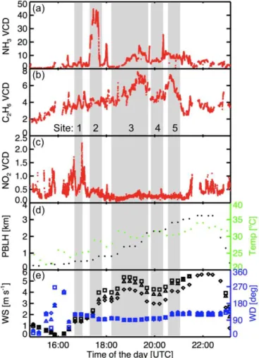
Figure 7.Time series of the VCDs (1016molec cm−2) measured for(a)NH3,(b)C2H6and(c)NO2during RD11.(d)PBLH and temperature.(e)Model wind speed and model wind direction aver-aged over approximately 10–50 m above ground level (diamonds), over half PBLH (triangles) and over the full PBLH (squares). Shaded areas indicate times at each site (numbers correspond to those in Fig. 6).
tancey,Z is the VCD of a gas of interest, andq is a scal-ing exponent (Harris et al., 2001; Follette-Cook et al., 2015). Settingq equal to 1 this structure function is a useful tool to quantify trace gas variability over horizontal distance. At small distances between measurements the structure func-tion exhibits the largest rate of change and increases until converging at larger distances. Variabilities increase as both plumes and background air masses are observed. At a cer-tain spatial distance the structure function converges against a maximum VCD variability. We define the variability length scale to determine over which spatial scales a certain per-centage of the maximum median variability is observed. The spatial distance at which the VCD variability is 50 % of the maximum variability is denoted asLV(50 %). Then LV(P )=d(P ·Vmax), (4)
whereLV denotes the variability length scale for a certain
percentageP andd(P ·Vmax)denotes the distance in
kilo-meters at which the VCD variability equalsP ·Vmax. Here, Vmaxis the maximum median variability.
Figure 9 shows the structure function with units of distance in kilometers on the abscissa, VCD difference has units of molecules cm−2on the ordinate, and a second ordinate scales the VCD difference with respect to the median VCD.
3 Results and discussion
3.1 Mobile SOF performance
3.1.1 Precision and accuracy
The LOD and precision of NO2 from the DS-DOAS
are 7×10¹⁴ and 3×10¹⁴molecules cm−2, respectively (Baidar et al., 2016). Figure 3 illustrates the data used to determine the LOD and accuracy of the CU mo-bile SOF. The absolute values of the difference between the VCDs averaged over identical time intervals mea-sured by the HR-NCAR-FTS and by the mobile SOF were used to quantify accuracy. The results are presented in Table 4. The findings for measurement precision and accuracy (compare Sect. 2.4, Eq. 1) result in the fol-lowing LODs: LODNH3=0.10×10
16molecules cm−2 and
LODC2H6 =0.13×10
16molecules cm−2. The accuracy is
the above given LOD values this means that the accu-racy is limiting the overall uncertainty in trace gas obser-vations at concentrations greater than 2.27×10¹⁶ for NH3
and 1.94×10¹⁶molecules cm−2for C2H6. During FRAPPE,
the VCDs were greater than the LOD in 99.98 % for NH3
and 100 % for C2H6 of the measurements, which means
the LOD was an issue in a low amount of measurements. In terms of the total error (see Table 4), this means that the uncertainty was determined by the accuracy of the ob-served median and maximum and the LOD was limiting the uncertainty on the minimum observed VCD. For a me-dian VCD of 4.32×10¹⁶molecules cm−2for NH3the
uncer-tainty is 0.19×10¹⁶molecules cm−2, and for a median VCD of 3.49×10¹⁶molecules cm−2 for C2H6 the uncertainty is
0.23×10¹⁶molecules cm−2.
3.1.2 Instrument line shape
While driving around a source area or site of interest there are 90◦ changes in the azimuth angle with each turn and many smaller degree changes in both elevation and azimuth angles due to fine tracking on uneven dirt roads. Column density measurements along the∼2.0 m long beam between the col-limated light source of a globar and the spectrometer at solar tracker azimuth angles from 0 to 360◦and at elevation angles of 5, 45 and 65◦were recorded to determine the ILS based on water vapor lines (compare Sect. 2.6). Figure 4 shows the modulation efficiency at maximum OPD as a function of az-imuth angle. The inner circle shows the measurements for the MCT detector; the outer circle shows the measurements for the InSb detector. Figure 5 shows both the modulation effi-ciency and phase error as a function of OPD. The top plots show the InSb results; the bottom plots show the MCT re-sults. It can be seen that the modulation efficiency of both detectors shows rather constant behavior. From these exper-iments it was determined that the MCT detector has a mod-ulation efficiency of 0.968 at maximum OPD and the InSb detector has a modulation efficiency of 1.010 at maximum OPD. These values are obtained by averaging the modulation efficiency at maximum OPD over all azimuth and elevation angle.
To investigate the effect of the ILS on the retrieval of NH3
and C2H6, the retrieval software was first run using an ideal
ILS as input and then using the ILS measured for the MCT and InSb detector, respectively, and comparing the VCD out-put with ideal and measured ILS. There was 0.5 % change in the retrieved NH3VCD and no change in the C2H6VCD.
These results are listed in Table 4 and are factored into the total error on VCDs. We conclude that there is no significant angular dependency on the ILS.
3.2 Mobile SOF deployment
The mobile SOF was deployed during 16 RDs during FRAPPE. Here, we present data from two RDs that were
conducted along almost identical drive tracks on consecu-tive days as well as shared common scientific objecconsecu-tives. The drive track for the case study from 13 August 2014 is shown in Fig. 6 and is similar to the drive track on 12 August 2014. The five sites indicated in that figure contain feedlots (and probably ONG storage tanks). On 12 and 13 August 2014, RD10 and RD11, respectively, the following median (minimum, maximum) VCDs were observed: 4.3 (0.5, 45) for NH3, 3.5 (1.5, 7.7) for C2H6 and 0.4 (0.06,
2.2)×1016molecules cm−2for NO2.
The variability in total column densities during RD11 is shown in Figs. 7 and 8. The identical figures for RD10 are included as Figs. S2 and S3. Both RDs show similar features in VCD enhancement (VCD – VCDbackground)of the gases,
temperature and wind. Figure 7 shows the VCD time series of the three gases, a time series for the temperature and PBLH, and the model wind speed and direction. NH3shows
signifi-cant column enhancement for site 2, which was the concen-trated animal feeding operation (CAFO) with∼54 000 cat-tle. NO2also shows some VCD enhancement for site 2.
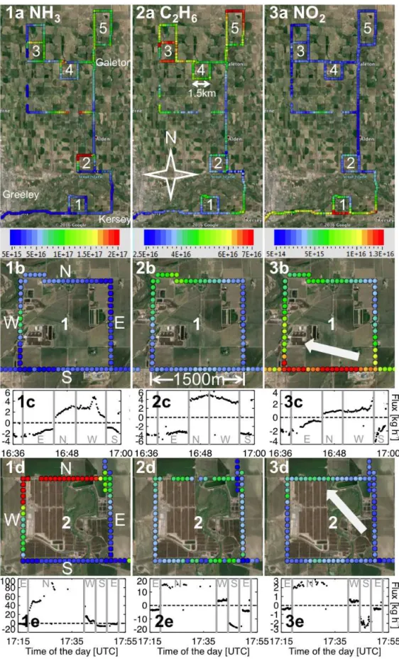
Fig-ure 8 shows the VCD time series in form of a Google Earth visualization to indicate the spatial distribution. Sites 1 and 2 are also shown enlarged to visualize the downwind and up-wind effects. Site 1 is a source for both NH3and C2H6. There
is a dairy farm located near the west end of the site and a source for C2H6in the upper right of the site. The VCD
en-hancement of NO2at the south leg of the site is due to heavy
traffic on that street. Site 2 for NH3shows the column
en-hancement downwind of the cattle feedlot and a background VCD upwind of the cattle feedlot. For that same site NO2
shows a larger column enhancement downwind than upwind. C2H6is mostly transported through site 2, as can be seen in
that the VCD is on the same color scale upwind and down-wind of site 2.
3.3 Emission fluxes
The emission fluxes were calculated according to Eq. (2) described in Sect. 2.5. The wind used for flux calculations has been averaged within the planetary boundary layer (see Fig. 7). Figure 8c and e show the flux as time series for each site. The stretch downwind of a site shows positive flux val-ues if the site is a source. If the site is not a source, and a gas is passing through the site, then the absolute value of nega-tive incoming flux and posinega-tive outgoing flux are expected to be comparable.
The calculated net fluxes are presented in Table 5 for RD10 and RD11. Particularly we could verify that cattle and dairy farms in sites 1, 2 and 4 are significant sources for NH3
and that the CAFO soil in site 2 is a significant source of NOx, which we observed in terms of a positive NO2
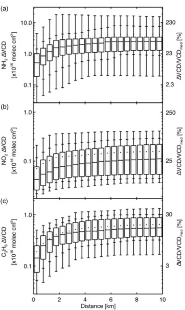
Figure 9.Structure functions of(a)NH3,(b)C2H6and(c)NO2 using data from RD11 with a time constraint of 30 min for the time period of the five sites. The bin width is 500 m. Boxes mark 25th and 75th percentiles, the dot indicates the mean and the line inside the box marks the median. Dashes below and above the boxes indicate 5th, 15th, 85th and 95th percentile.
these error bars. The individual gas fluxes are discussed in the following three subsections.
3.3.1 NH3fluxes
For sites 1, 2 and 4, the dairy and cattle feedlots are a source of NH3 during both RDs. The emission flux in site
2 with the largest head count of cattle shows agreement of better than 10 % for RD10 and RD11. The average flux is 649±24 kgNH3h−1for 54 044 cattle. This consistency
be-tween two days gives confidence that the uncertainty in the wind is conservatively estimated here. The average emis-sion factor for site 2 is 12.0±2.8 gNH3h−1head−1for both
days during daytime in the summer. The uncertainty here
combines the day-to-day variability and error in the wind (taken as 30 %/√2). For the dairy farm in site 4 we ob-tain 11.4±3.5 gNH3h−1head−1. The per head emission flux
from the two samples at site 2 and one sample at site 4 can be pooled resulting in an average emission factor of 11.8±2.1 gNH3h−1head−1. The head count for site 1 was
unknown but can be estimated based on the pooled per head emission. The average emission flux from site 1 of 108 kg h−1 corresponds to∼9200 cattle. During RD11 the upwind effect influenced the observed VCD at site 4 and precluded quantification of a flux. This means the upwind flux was significant, and variability during the course of driv-ing around the site may have influenced the observed flux. A comparison of the determined NH3fluxes to literature values
is given in Sect. 3.4.1.
3.3.2 NO2production rates
Soils are sources of NOx, which is primarily emitted as NO
as a result of microbial activity (Zörner et al., 2016). NO2is
subsequently produced from the reaction NO+O3→NO2+
O2 in the atmosphere. Both RDs consistently showed site
2 is a significant source of NOx, with an average
mea-sured NO2 production rate of 14.5 kg h−1. The difference
in the NO2emission flux from 18 kg h−1during RD10 and
11 kg h−1 during RD11 may represent differences in wind speed. During RD10 the wind speed was approximately 1 to 2 m s−1slower than on RD11 (compare Figs. 7 and S2), allowing for less time for NO into NO2 conversion during
transport. The reaction rate constant for the above reaction is
k=3.0×10⁻¹²
×e−1500/T cm3molec−1s−1(Sander et al.,
2006), which at a temperature of 300 K corresponds to a value for the rate constant of 2.02×10⁻¹⁴cm3molec−1s−1
during our case studies. On RD10 and RD11 O3
concen-trations of 64 and 68 ppb at 19:00 and 18:00 UTC, respec-tively (Pierce, 2016), correspond to a NO lifetime of∼40 s (66 ppbv O3). With wind speeds of ∼4 m s−1 NO was
converted into NO2 over a distance of ∼160 m (RD11).
In particular, there is sufficient time to convert most of the NO emissions into NO2 within the CAFO area of
1.6×1.6 km2. To estimate the NO2/NO ratio under
pho-tostationary state, we also need to consider the photochem-ical destruction of NO2from the reaction NO2+O2→(hv)
NO+O3. Assuming a typical photolysis frequency, J(NO2),
as∼8×10⁻³s−1, the NO
2/NO ratio is 3.6, indicating that
∼80 % of NOx is abundant as NO2. The average measured
NO2production rate thus corresponds to a NOxemission rate
of 18.6±7.4 kg h−1for site 2. For a fraction of the nearby
soil emission there may not be sufficient time to reach the photochemical steady state, but this fraction is likely small. We conclude that the observed NO2 is a lower limit for the
overall NOx production. The NOx flux is compared to the
emission inventory (EPA, 2015) in Sect. 3.4.2.
We are able to determine that the NOxis coming from the
genera-3.3.3 C2H6fluxes
C2H6 has a relatively long atmospheric lifetime of
about 2 months and is lost in the reaction with OH: OH+C2H6→C2H5+ H2O. Assuming an OH
concentra-tion of 8×10⁶molecules cm−3and taking the OH reaction rate constant of 2.4×10⁻¹³cm3molec−1s−1(Sander et al., 2006), the lifetime of C2H6is 60 days, which gives rise to
a Northern Hemisphere (NH) background VCD of, for ex-ample, 3.1×10¹⁶molecules cm−2 at Kiruna, Sweden
(An-gelbratt et al., 2011). C2H6 VCD enhancements over the
NH background are therefore expected to mix on regional scales and are subject to significant transport in the atmo-sphere. The RDs measured the lowest VCDs of C2H6 in
Boulder County, CO with its moratorium on fracking. En-hanced VCDs were observed throughout Weld County, CO, in areas with active ONG production. Using all 16 RDs, the median (minimum, maximum) VCDs in Boulder County and Weld County were 1.5 (0.5, 3.1)×1016 and 3.5 (1.0, 10)×1016molecules cm−2, respectively. The influence from upwind sources makes the quantification of C2H6 emission
fluxes a bit more challenging. We consistently were able to quantify a positive emission flux out of site 1, as shown in Table 5. Site 1 was also influenced from upwind sources, but the mean C2H6flux was calculated as 63.5 kg h−1with
an uncertainty of 29 kg h−1. The C
2H6 flux is compared to
the emission inventory (EPA 2015) in Sect. 3.4.3.
3.4 Comparison with literature values
3.4.1 NH3fluxes from CAFO
We compare the NH3 per head emission rate from cattle
and dairy with literature values in Table 6. In Sect. 3.3.1 we calculated the emission rate of NH3 for cattle to be
11.8±2.1 g h−1head−1 based on the beef and dairy farm estimated capacity and observed NH3VCDs. Notably, it is
not guaranteed that during the RD the feedlot was at maxi-mum occupancy. If the occupancy was lower than the max-imum occupancy, the value of 11.8 g h−1head−1 would be
a lower limit of the actual per head emission rate. The area of site 2 is mostly covered by two cattle feedlots, such that the likelihood of measuring NH3 from another source such
as fertilizers is low. The comparison with literature values in Table 6 shows that our per head emission factor of NH3
is near the upper range of reported values and higher by a factor of 1.1 to 8.9. Plausible explanations may be due
colder temperatures (Bjorneberg et al., 2009), suggesting that factors other than temperature contribute to the significant variability among literature values.
Additionally we compare the NH3emission flux with the
NEI 2011 emission inventory (EPA, 2015). The inventory has been formatted to a 3 km WRF-Chem grid, and the emis-sions for July 2011 are given as hourly intervals and do not distinguish between different source sectors. Agricul-ture is responsible for the major share of NH3emissions in
the Colorado Front Range. For Fig. S4 the maximum emis-sion flux from the diurnal profile in NEI 2011 was extracted corresponding to 0.73 kg km−2h−1 at 20:00 UTC, in order to make a conservative comparison with the measured NH3
emission rates. For comparison, the 16:00–22:00 UTC aver-age NEI 2011 emission flux is 0.71 kg km−2h−1. We com-pare the emission flux of NH3 in several ways. The first
approach is to use Weld County, where the emission in-ventory suggests an average NH3flux of 0.36 kg km−2h−1
for the maximum daytime emissions during summer. Based on our average per head emission factor, and a maximum head count of 535 766 cattle from beef and dairy feedlots in Weld County in 2014 (D. Bon, 2016, personal commu-nication), the NH3 emission flux is 0.63 kg km−2h−1. That
means that the EPA (2011) inventory underestimates the NH3
emission for the total county by about a factor of 2. Focus-ing on the area within Weld County, containFocus-ing the five sites probed during our RDs, the inventory suggests the NH3
emis-sion flux is 0.73 kg km−2h−1 compared to the NH3flux of
6.39 kg km−2h−1based on head count within the area. This represents an underestimation by a factor of about 10. The differences with the NEI are estimated conservatively here and could be lower limits if other NH3sources were located
within the county, but not captured by our measurements, or if the CAFOs probed were not a maximum capacity. The emission inventory is from a few years prior to the RDs, and the total emission of the feedlots may have increased, as may have the number of feedlots within the grid cells. The 2007 Census of Agriculture for Weld County indicates 565 327 as number of cattle and calves, the 2012 Census indicates 501 446, and for 2014 the capacity was 535 766. Even if the number of feedlots within individual grid cells changed, the capacity did not change by more than 12 %, which does not describe the underestimation of NH3emission that we
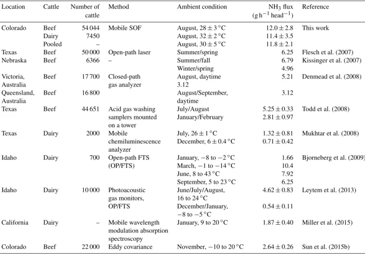
Table 6.Comparison of NH3emission rates from cattle with literature values.
Location Cattle Number of Method Ambient condition NH3flux Reference
cattle (g h−1head−1)
Colorado Beef 54 044 Mobile SOF August, 28±3◦C 12.0±2.8 This work
Dairy 7450 August, 32±2◦C 11.4±3.5
Pooled – August, 30±5◦C 11.8±2.1
Texas Beef 50 000 Open-path laser Summer/spring 6.25 Flesch et al. (2007)
Nebraska Beef 6366 – Summer/fall 6.79 Kissinger et al. (2007)
Winter/spring 4.96
Victoria, Beef 17 700 Closed-path August, daytime 5.21 Denmead et al. (2008)
Australia gas analyzer 3.12
Queensland, Beef 16 800 August/September, 3.12
Australia daytime
Texas Beef 44 651 Acid gas washing July/August 5.25±0.33 Todd et al. (2008) samplers mounted January/February 2.81±0.97
on a tower
Texas Dairy 2000 Mobile July, 26±1◦C 1.32±0.81 Mukhtar et al. (2008)
chemiluminescence December, 6±0.4◦C 0.71±0.42 analyzer
Idaho Dairy 700 Open-path FTS January,−8 to−2◦C 1.66 Bjorneberg et al. (2009)
(OP/FTS) March,−1 to−14◦C 10.4
June, 8 to 43◦C 7.92
September, 5 to 23◦C 6.25
Idaho Dairy 10 000 Photoacoustic June/July/August, 4.62±0.83 Leytem et al. (2013) gas monitors, 16 to 24◦C
OP/FTS December/January, 0.54±0.11
−8 to−5◦C
California Dairy – Mobile wavelength January, 9 to 20◦C 1.87±0.40 Miller et al. (2015) modulation absorption
spectroscopy
Colorado Beef 22 000 Eddy covariance November,−10 to 20◦C 2.64±0.26 Sun et al. (2015b)
We conclude that using the NEI 2011 emission inventory in air quality models most likely underestimates the actual NH3
emissions during FRAPPE by a factor of 2–10.
3.4.2 NOxemissions from CAFO
We have consistently observed significant NOx emissions
from CAFO with a rate of 7.3±2.9 kg km−2h−1 from site 2, or 18.6 kg h−1 during both RDs. No sharp plumes were observed downwind of the site (see Figs. 7c, 8-2d, and Figs. S2c, S3-2d). The NO2 column enhancements closely
resemble the area of cattle feeding operations, which sug-gests the observed NOx is emitted from microbial
activ-ity in the CAFO soils rather than a stationary combustion source. In order to assess the potential relevance of the en-hanced soil emissions of NOx from CAFOs for the
over-all NOx emissions in Weld County, we determine the NOx
production rate for cattle as 0.34 g h−1head−1 from site 2. Notably, the fact that we did not observe NOx emissions
from other sites is compatible with this assumption. At the feedlot in site 4 we were not able to obtain a reproducible flux on RD10 and RD11; instead, the emission was slightly positive on RD10 and negative on RD11 due to an upwind
plume affecting the measurements (see Table 5). Using the per head NOx flux as determined based on site 2, the NOx
flux for site 4 would have been 2.5 kg h−1compared to the average NOxflux of 1.7±0.5 kg h−1during RD10. There is
thus reasonable agreement if the difference in the CAFO ca-pacity is accounted for. Based on the total count of 533 766 cattle in Weld County and an area of 10 404 km2 we ob-tain an average contribution from CAFO soil emissions of 0.018 kg km−2h−1. The inventory produces a NOx flux of
0.17 kg km−2h−1averaged over Weld County (EPA 2015), which includes emissions from urban areas. We conclude that the NOx source associated with enhanced microbial
activ-ity in CAFO soils could potentially contribute∼10 % to the overall NOxemissions of Weld County.
The contribution is even higher in the remote area of the five sites probed during the RDs. Here, the inventory pro-duces an average NOx flux of 0.15 kg km−2h−1. Based on
the total count of 224 469 cattle in the CAFOs distributed over the area of 414 km2 shown in the bottom panel of Fig. S4, the NOx source from CAFO soils corresponds to
0.18 kg km−2h−1. We conclude that the CAFO soil emis-sions can double the NOxsource in the inventory in the area
from the CU mobile SOF spectra, which hold potential to complement the NO2VCD observations in the future.
3.4.3 C2H6emissions
We determined that the C2H6 emission for site 1 is
63.5±29 kg h−1. The NEI 2011 emission inventory (EPA,
2015) estimates the C2H6 emission for that area as
2.39 kg km−2h−1. Scaling our emission rate to the area
of that one 9 km2 grid cell of the inventory, we obtain ∼7 kg km−2h−1from site 1. While these measurements in-dicate the capability of mobile SOF to quantify elevated fluxes of C2H6, possibly from leaks, this flux is likely not
representative of the greater area of the county. The CU mo-bile SOF C2H6measurements obtained on a regional scale
are most useful if combined with a regional-scale chemistry transport model or inverse model to estimate the C2H6
emis-sions in the Colorado Front Range. From in situ observations the ratio of C2H6/CH4for ONG emissions in Weld County
has been measured as 18.4 % (A. Fried, personal communi-cation, 2014), 11 % (A. Townsend-Small, personal commu-nication, 2014) and 10 % (T. Yacovitch, personal communi-cation, 2014). Based on the average ratio of 13.1±4.6 % and the emission flux for C2H6, the CH4emission flux is 39.2–
82.7 kg km−2h−1at site 1.
3.5 Spatial variability
The structure function for the NH3, NO2 and C2H6 VCDs
are shown in Fig. 9. We applied a time constraint of 30 min to calculate the structure functions (compare Sect. 2.6, Eq. 3), in order to minimize changes in atmospheric state due to trans-port. Over the first few bins column differences in plumes are small due to measurements being in close vicinity of each other. At greater distances column differences increase and converge onto a plateau that is determined by the variability between plumes and background air masses.
During RD10 and RD11 we observed the highest spatial variability for NH3, somewhat lower variability for NO2,
and the smallest variability for C2H6VCDs. The observed
plateau values were 2.52×10¹⁶ for NH3, 0.13×10¹⁶ for
NO2and 0.57×10¹⁶molecules cm−2for C2H6, which
cor-respond to 58.6, 32.5 and 16.3 % of the median VCD for NH3, NO2 and C2H6, respectively. These plateau values
should be viewed as specific for our study area, and they may differ significantly for urban areas, where the sources may be more distributed.
aLength at which 50 % of the variability with respect to the
median VCD occurs.bLength at which 90 % of the variability with respect to the median VCD occurs.cLength scale at which the VCD difference is equal to the value of the LOD.
The precision of our NH3and C2H6measurements, given
in Table 4, determines how well we can resolve variability in VCDs. If the VCD difference is smaller than the measure-ment precision, then the VCD differences may be insignif-icant within our measurement precision. While the mobile SOF probed VCDs at spatial resolution of 5–19 m, we are able to resolve significant variability on spatial scales greater than 25 m for all gases. The variability length scales (see Sect. 2.6, Eq. 4) of NH3, NO2 and C2H6 for 50 and 90 %
variability as well as the length scale near the LOD are given in Table 7. The 50 and 90 % variability length scales are sim-ilar for all gases despite their different plateau values, with
LV (50 %) occurring at distances well below 2 km and LV
(90 %) occurring at distances near and below 6 km.
The feedlots in sites 1, 2 and 4 which are sources for NH3
have a minimum width of 400 m for site 1 and 4 and 800 m for site 2. Our results are thus consistent with the expected plume diameters in close vicinity to these sites.
The current satellites measuring NH3 have a
horizon-tal resolution of 5.3×8.5 (TES) and 12×25 km2 (IASI). Satellites measuring NO2 have a horizontal resolution of
13×24 (OMI), 40×80 (GOME2) and 15×26 km2 (SCIA-MACHY). The expected resolution of TEMPO (Tropo-spheric Emissions: Monitoring of Pollution), to be launched in 2019, from geostationary orbit is 2×4.5 km2. We observe significant variability, > 90 %, in VCDs at variability length scales smaller than∼6 km for NH3and C2H6, and∼13 km
for NO2 (Table 7). This indicates that satellites are able to
quantify 10 % of the total variability in VCDs. Future satel-lites such as TEMPO and GEMS have a horizontal resolution that will begin to approach the scales over which NO2VCDs
vary by 50 % in the atmosphere, though some averaging from limited grid-size resolution can still be expected.
4 Conclusion and outlook
We describe the CU mobile SOF instrument, character-ize it, and demonstrate first applications to charactercharacter-ize structure functions and quantify emission fluxes of NH3,
NOx and C2H6. The instrument can be extended to
acid (HONO), hydrogen cyanide (HCN), acetylene (C2H2),
methanol (CH3OH), formic acid (HCOOH), formaldehyde
(HCHO), glyoxal (C2H2O2), ozone (O3), among others.
We conclude that mobile SOF measurements of trace gas VCDs are complementary to in situ observations, eliminate assumptions about vertical distributions and allow for a more direct comparison with satellites. Also, the FTS is well suited to detect typical VCDs in the Colorado Front Range with ex-cellent signal to noise ratio. The NH3, NO2and C2H6VCDs
were above the instrument detection limit in 99.98, 95.89 and 100 % of the spectra, respectively. The CU mobile SOF in-strument line shape is not affected by changes in azimuth or elevation angles, providing robust spectral retrievals also while driving on dirt roads or around corners.
The total VCD error is 4.4 % for NH3, 6.7 % for C2H6and
5 % for NO2at high signal to noise ratio, and the accuracy
is 0.10×10¹⁶ for NH3 and 0.13×10¹⁶molecules cm−2for
C2H6. The error limiting the spectroscopic measurement is
the cross section uncertainty. The uncertainty in the flux cal-culations is limited by the knowledge about the winds, con-sistent with earlier conclusions (Mellqvist et al., 2010). De-termination of the spatial variability and structure function is not limited by the instrument precision, unless at very low distances shorter than 25 m. This is similar to earlier findings for in situ data (Follette-Cook et al., 2015).
Significant variability in the VCDs is observed for all gases on scales smaller than 6 km, and we found 50 % of the VCD variability was at distances shorter than 2 km. Most of this variability happens on scales smaller than current ground pixel sizes of satellites. At the available spatial resolutions, satellites currently quantify less than 10 % of the observed VCD variability. Future missions from geostationary orbit, such as TEMPO, GEMS and Sentinel4, will have smaller ground pixels, which can resolve 10 to < 50 % of the vari-ability observed in the NO2VCDs.
A regional gradient was observed for C2H6between
Boul-der County and Weld County. The median, minimum and maximum C2H6 VCDs were 2–3 times larger in Weld
County, consistent with the active ONG extraction here and a moratorium on fracking in Boulder County (in 2014).
Emission fluxes for NH3during the summer day time are
generally underestimated in the NEI 2011 emission inven-tory, as well as NOx emissions from CAFO soil. This
indi-cates there are sources that have not been accounted for in the inventory. We determined that the per head emission of NH3during two summer days is underestimated by a factor
of 2–10 than determined by other literature and the emission inventory. Emissions of NOx from microbiological activity
in CAFO soils account for∼10 % of the total NOxemission
in Weld County, CO, and can double the NOxsource in the
rural agricultural areas studied.
The CU mobile SOF instrument provides a versatile, ef-ficient and robust tool to improve the statistics of emission fluxes of NH3, NOxand C2H6as there are no losses in
sam-pling lines, study emissions of other gases and study
vari-ations in emissions with temperature, in different seasons, from point and area sources inside and outside of Colorado. The quality of the emission flux estimates benefits from inde-pendent wind measurements and closer attention to upwind effects in particular for C2H6. The airborne deployment of
the CU mobile SOF instrument is planned for summer 2016 and has the potential to make mobile SOF measurements in-dependent of roads, which is of interest to the studies in more complex terrain, such as of biomass burning events.
List of primary chemicals and acronyms
C2H6– ethane
HCHO – formaldehyde NH3– ammonia
NO2– nitrogen dioxide
NOx– sum of nitric oxide (NO) and NO2
CAFO – concentrated animal feeding operation CLD – center to limb darkening
CU – University of Colorado
DOAS – differential optical absorption spectroscopy DS-DOAS – direct-sun DOAS
EPA – Environmental Protection Agency
FRAPPE – Front Range Air Pollution and Photochemistry Experiment
FTS – Fourier transform spectrometer
HR-NCAR-FTS – high-resolution FTS at the National Cen-ter for Atmospheric Research
ILS – instrument line shape InSb – indium antimonide IR – infrared
LOD – limit of detection MAX-DOAS – multi-axis DOAS MCT – mercury cadmium telluride NEI – National Emission Inventory ONG – oil and natural gas
OPD – optical path difference
PBLH – planetary boundary layer height RD – research drive
SOF – Solar Occultation Flux UV–vis – ultraviolet–visible VCD – vertical column density
5 Data availability
Rainer Volkamer conducted the measurements; Philip Hand-ley and Owen R. Cooper helped during the field deploy-ment; Owen R. Cooper, Frank Hase, James W. Hannigan and Gabriele Pfister added tools and expertise during analysis; Na-talie Kille and Sunil Baidar analyzed the data; NaNa-talie Kille and Rainer Volkamer prepared the manuscript with contributions from all co-authors.
Competing interests. The authors declare that they have no conflict of interest.
Acknowledgements. Financial support from Colorado Department for Public Health and Environment (CDPHE), State of Colorado contract 14 FAA 64390 and National Science Foundation (NSF) EAGER grant AGS-1452317 is gratefully acknowledged. The solar tracker was developed with support from a CIRES Energy Initiative seed grant. The authors thank Daniel Bon from CDPHE for providing the inventory of feedlot capacities during FRAPPE, Eric Nussbaumer for the SFIT4 software, Melanie Follette-Cook for sharing code and helpful discussions, and Tom Ryerson for coordinating research drives. Natalie Kille is recipient of a CIRES graduate fellowship. Rainer Volkamer is recipient of a KIT Distinguished International Scholar award. We acknowledge support by Deutsche Forschungsgemeinschaft and Open Access Publishing Fund of KIT. NCAR is sponsored by the NSF.
Edited by: M. Hamilton
Reviewed by: M. K. Sha and two anonymous referees
References
Ahmadov, R., McKeen, S., Trainer, M., Banta, R., Brewer, A., Brown, S., Edwards, P. M., de Gouw, J. A., Frost, G. J., Gilman, J., Helmig, D., Johnson, B., Karion, A., Koss, A., Langford, A., Lerner, B., Olson, J., Oltmans, S., Peischl, J., Pétron, G., Pichugina, Y., Roberts, J. M., Ryerson, T., Schnell, R., Senff, C., Sweeney, C., Thompson, C., Veres, P. R., Warneke, C., Wild, R., Williams, E. J., Yuan, B., and Zamora, R.: Understanding high wintertime ozone pollution events in an oil- and natural gas-producing region of the western US, Atmos. Chem. Phys., 15, 411–429, doi:10.5194/acp-15-411-2015, 2015.
Angelbratt, J., Mellqvist, J., Simpson, D., Jonson, J. E., Blumen-stock, T., Borsdorff, T., Duchatelet, P., Forster, F., Hase, F., Mahieu, E., De Mazière, M., Notholt, J., Petersen, A. K., Raffal-ski, U., Servais, C., Sussmann, R., Warneke, T., and Vigouroux, C.: Carbon monoxide (CO) and ethane (C2H6) trends from
British Journal for Environmental and Climate Change, 3, 566– 586, doi:10.9734/BJECC/2013/5740, 2013.
Baidar, S., Kille, N., Ortega, I., Sinreich, R., Thomson, D., Hanni-gan, J., and Volkamer, R.: Development of a digital mobile so-lar tracker, Atmos. Meas. Tech., 9, 963–972, doi:10.5194/amt-9-963-2016, 2016.
Baum, K. A., Ham, J. M., Brunsell, N. A., and Coyne, P. I.: Surface boundary layer of cattle feedlots: Implications for air emissions measurement, Agr. Forest Meteorol., 148, 1882–1893, doi:10.1016/j.agrformet.2008.06.017, 2008.
Bertram, T. H., Heckel, A., Richter, A., Burrows, J. P., and Cohen, R. C.: Satellite measurements of daily variations in soil NOx emissions, Geophys. Res. Lett., 32, L24812,
doi:10.1029/2005GL024640, 2005.
Bjorneberg, D. L., Leytem, A. B., Westermann, D. T., Grif-fiths, P. R., Shao, L., and Pollard, M. J.: Measurement of At-mospheric Ammonia, Methane, and Nitrous Oxide at a Con-centrated Dairy Production Facility in Southern Idaho Using Open-Path FTIR Spectrometry, T. ASABE, 52, 1749–1756, doi:10.13031/2013.29137, 2009.
Boersma, K. F., Jacob, D. J., Trainic, M., Rudich, Y., DeSmedt, I., Dirksen, R., and Eskes, H. J.: Validation of urban NO2 concen-trations and their diurnal and seasonal variations observed from the SCIAMACHY and OMI sensors using in situ surface mea-surements in Israeli cities, Atmos. Chem. Phys., 9, 3867–3879, doi:10.5194/acp-9-3867-2009, 2009.
Carslaw, D. C. and Beevers, S. D.: Estimations of road ve-hicle primary NO2 exhaust emission fractions using mon-itoring data in London, Atmos. Environ., 39, 167–177, doi:10.1016/j.atmosenv.2004.08.053, 2005.
Chen, J., Viatte, C., Hedelius, J. K., Jones, T., Franklin, J. E., Parker, H., Gottlieb, E. W., Wennberg, P. O., Dubey, M. K., and Wofsy, S. C.: Differential column measurements using compact solar-tracking spectrometers, Atmos. Chem. Phys., 16, 8479–8498, doi:10.5194/acp-16-8479-2016, 2016.
Coheur, P.-F., Herbin, H., Clerbaux, C., Hurtmans, D., Wespes, C., Carleer, M., Turquety, S., Rinsland, C. P., Remedios, J., Hauglus-taine, D., Boone, C. D., and Bernath, P. F.: ACE-FTS observation of a young biomass burning plume: first reported measurements of C2H4, C3HO, H2CO and PAN by infrared occultation from space, Atmos. Chem. Phys., 7, 5437–5446, doi:10.5194/acp-7-5437-2007, 2007.
de Foy, B., Lei, W., Zavala, M., Volkamer, R., Samuelsson, J., Mel-lqvist, J., Galle, B., Martínez, A.-P., Grutter, M., Retama, A., and Molina, L. T.: Modelling constraints on the emission inventory and on vertical dispersion for CO and SO2in the Mexico City Metropolitan Area using Solar FTIR and zenith sky UV spec-troscopy, Atmos. Chem. Phys., 7, 781–801, doi:10.5194/acp-7-781-2007, 2007.
De Gouw, J. A., Te Lintel Hekkert, S., Mellqvist, J., Warneke, C., Atlas, E. L., Fehsenfeld, F. C., Fried, A., Frost, G. J., Harren, F. J. M., Holloway, J. S., Lefer, B., Lueb, R., Meagher, J. F., Parrish, D. D., Patel., M., Pope, L., Richter, D., Rivera, C., Ryerson, T. B., Samuelsson, J., Walega, J., Washenfelder, R. A., Weibring, P., and Zhu, X.: Airborne Measurements of Ethene from Industrial Sources Using Laser Photo-Acoustic Spectroscopy, Environ. Sci. Technol., 43, 2437–2442, doi:10.1021/es802701a, 2009. Denmead, O. T., Chen, D., Griffith, D. W. T., Loh, Z. M., Bai, M.,
and Naylor, T: Emissions of the indirect greenhouse gases NH3 and NOxfrom Australian beef cattle feedlots, Aust. J. Exp. Agr.,
48, 213–218, 2008.
Doyle, G. J., Tuazon, E. C., Graham, R. A., Mischke, T. M., Winer, A. M., and Pitts Jr., J. N.: Simultaneous concentrations of ammo-nia and nitric acid in a polluted atmosphere and their equilibrium relationship to particulate ammonium nitrate, Environ. Sci. Tech-nol., 13, 1416–1419, doi:10.1021/es60159a010, 1979.
Environmental Protection Agency (EPA): 2011 National Emission Inventory version 2, 2015.
EPA Handbook: Optical Remote Sensing for Measurement and Monitoring of Emissions Flux, edited by: Mikael, D. K., Of-fice of Air Quality Planning and Standards, Air Quality Anal-ysis Division Measurement Technology Group, Research Trian-gle, North Carolina, 27711, 2011.
European Commision: Best Available Technique (BAT) Refer-ence Document for the Refining of Mineral Oil and Gas: Joint Research Centre, Institute for Prospective Technolog-ical Studies, ISBN 978-92-79-46198-9, ISSN 1831-9424, doi:10.2791/010758, 2015.
Fangmeier, A., Hadwiger-Fangmeier, A., Van der Eerden, L., and Jäger, H.-J.: Effects of Atmospheric Ammonia on Vegetation – A Review, Environ. Pollut., 86, 43–82, doi:10.1016/0269-7491(94)90008-6, 1994.
Finlayson-Pitts, B. J. and Pitts Jr., J. N.: Chemistry of the Upper and Lower Atmosphere, Academic Press, San Diego, CA, 882–886, 2000.
Fischer, H., Birk, M., Blom, C., Carli, B., Carlotti, M., von Clar-mann, T., Delbouille, L., Dudhia, A., Ehhalt, D., EndeClar-mann, M., Flaud, J. M., Gessner, R., Kleinert, A., Koopman, R., Langen, J., López-Puertas, M., Mosner, P., Nett, H., Oelhaf, H., Perron, G., Remedios, J., Ridolfi, M., Stiller, G., and Zander, R.: MIPAS: an instrument for atmospheric and climate research, Atmos. Chem. Phys., 8, 2151–2188, doi:10.5194/acp-8-2151-2008, 2008. Flesch, T. K., Wilson, J. D., Harper, L. A., Todd, R. W., and Cole, N.
A.: Determining ammonia emissions from a cattle feedlot with an inverse dispersion technique, Agr. Forest Meteorol., 144, 139– 155, doi:10.1016/j.agrformet.2007.02.006, 2007.
Follette-Cook, M. B., Pickering, K. E., Crawford, J. H., Duncan, B. N., Loughner, C. P., Diskin, G. S., Fried, A., and Weinheimer, A. J.: Spatial and temporal variability of trace gas columns derived from WRF/Chem regional model output: Planning for
geosta-tionary observations of atmospheric composition, Atmos. Envi-ron., 118, 28–44, doi:10.1016/j.atmosenv.2015.07.024, 2015. Franco, B., Hendrick, F., Van Roozendael, M., Müller, J.-F.,
Stavrakou, T., Marais, E. A., Bovy, B., Bader, W., Fayt, C., Her-mans, C., Lejeune, B., Pinardi, G., Servais, C., and Mahieu, E.: Retrievals of formaldehyde from ground-based FTIR and MAX-DOAS observations at the Jungfraujoch station and com-parisons with GEOS-Chem and IMAGES model simulations, At-mos. Meas. Tech., 8, 1733–1756, doi:10.5194/amt-8-1733-2015, 2015.
Fried, A., McKeen, S., Sewell, S., Harder, J., Henry, B., Goldan, P., Kuster, W., Williams, E., Baumann, K., Shetter, R., and Cantrell, C.: Photochemistry of formaldehyde during the 1993 Tropo-spheric OH Photochemistry Experiment, J. Geophys. Res., 102, 6283–6296, doi:10.1029/96JD03249, 1997.
Glatthor, N., von Clarmann, T., Stiller, G. P., Funke, B., Kouk-ouli, M. E., Fischer, H., Grabowski, U., Höpfner, M., Kellmann, S., and Linden, A.: Large-scale upper tropospheric pollution observed by MIPAS HCN and C2H6 global distributions, At-mos. Chem. Phys., 9, 9619–9634, doi:10.5194/acp-9-9619-2009, 2009.
Harris, D., Foufoula-Georgiou, E., Droegemeier, K. K., and Levit, J. J.: Multiscale statistical properties of a high resolution precip-itation forecast, J. Hydrometeorol., 2, 406–418, 2001.
Harrison, J. J., Allen, N. D. C., and Bernath, P. F.: In-frared absorption cross sections for ethane (C2H6) in the 3 µm region, J. Quant. Spectrosc. Ra., 111, 357–363, doi.org/10.1016/j.jqsrt.2009.09.010, 2010.
Hase, F., Blumenstock, T., and Paton-Walsh, C.: Analysis of the instrumental line shape of high-resolution Fourier transform IR spectrometers with gas cell measurements and new retrieval soft-ware, Appl. Opt., 38, 3417–3422, doi:10.1364/AO.38.003417, 1999.
Hase, F., Hannigan, J. W., Coffey, M. T., Goldman, A., Höpfner, M., Jones, N. B., Rinsland, C. P., and Wood, S. W.: Intercompar-ison of retrieval codes used for the analysis of high-resolution, ground-based FTIR measurements, J. Quant. Spectrosc. Ra., 87, 25–52, doi:10.1016/j.jqsrt.2003.12.008, 2004.
Hase, F., Frey, M., Blumenstock, T., Groß, J., Kiel, M., Kohlhepp, R., Mengistu Tsidu, G., Schäfer, K., Sha, M. K., and Orphal, J.: Application of portable FTIR spectrometers for detecting green-house gas emissions of the major city Berlin, Atmos. Meas. Tech., 8, 3059–3068, doi:10.5194/amt-8-3059-2015, 2015. Höpfner, M., Volkamer, R., Grabowski, U., Grutter, M., Orphal,
J., Stiller, G., von Clarmann, T., and Wetzel, G.: First de-tection of ammonia (NH3) in the Asian summer monsoon upper troposphere, Atmos. Chem. Phys., 16, 14357–14369, doi:10.5194/acp-16-14357-2016, 2016.
Hristov, A. N., Hanigan, M., Cole, A., Todd, R., McAllister, T. A., Ndegwa, P. M., and Rotz, A.: Review: Ammonia emissions from dairy farms and beef feedlots, Can. J. Anim. Sci., 91, 1–35, doi:10.4141/CJAS10034, 2011.
Hutchinson, G. L., Mosier, A. R., and Andre, C. E.: Ammonia and Amine Emissions from a Large Cattle Feedlot, J. Environ. Qual., 11, 288–293, doi:10.2134/jeq1982.00472425001100020028x, 1982.