www.atmos-chem-phys.net/14/675/2014/ doi:10.5194/acp-14-675-2014
© Author(s) 2014. CC Attribution 3.0 License.
Atmospheric
Chemistry
and Physics
The impact of satellite-adjusted NO
x
emissions on simulated NO
x
and O
3
discrepancies in the urban and outflow areas of the Pacific
and Lower Middle US
Y. Choi
Department of Earth and Atmospheric Sciences,University of Houston, 312 Science & Research Building 1, Houston, TX 77204, USA
Correspondence to:Y. Choi ([email protected])
Received: 12 June 2013 – Published in Atmos. Chem. Phys. Discuss.: 13 August 2013 Revised: 28 November 2013 – Accepted: 14 December 2013 – Published: 22 January 2014
Abstract.We analyze the simulation results from a CMAQ model and GOME-2 NO2 retrievals over the United States for August 2009 to estimate the model-simulated biases of NOx concentrations over six geological re-gions (Pacific Coast = PC, Rocky Mountains = RM, Lower Middle = LM, Upper Middle = UM, Southeast = SE, North-east = NE). By comparing GOME-2 NO2 columns to cor-responding CMAQ NO2 columns, we produced satellite-adjusted NOx emission (“GOME2009”) and compared baseline emission (“BASE2009”) CMAQ simulations with GOME2009 CMAQ runs. We found that the latter exhib-ited decreases of−5.6 %,−12.3 %,−21.3 %, and−15.9 % over the PC, RM, LM, and SE regions, respectively, and increases of +2.3 % and +10.0 % over the UM and NE re-gions. In addition, we found that changes in NOx emis-sions generally mitigate discrepancies between the surface NOxconcentrations of baseline CMAQ and those of AQS at EPA AQS stations (mean bias of+19.8 % to −13.7 % over
PC, −13.8 % to −36.7 % over RM, +149.7 % to −1.8 %
over LM,+22.5 % to−7.8 % over UM,+31.3 % to−7.9 %
over SE, and+11.6 % to+0.7 % over NE). The relatively
high simulated NOx biases from baseline CMAQ over LM (+149.7 %) are likely the results of over-predictions of sim-ulated NOxemissions, which could shed light on those from global/regional Chemical Transport Models.
We also perform more detailed investigations on surface NOx and O3 concentrations in two urban and outflow ar-eas, PC (e.g., Los Angeles, South Pasadena, Anaheim, La Habra and Riverside) and LM (e.g., Houston, Beaumont and Sulphur). From two case studies, we found that the
information critical to establishing strategies for mitigating air pollution.
1 Introduction
Nitrogen oxides (NOx= NO + NO2) are major O3 precur-sors that originate from fossil fuel combustion, lightning, soil, aircraft, and biomass burning. The largest source of NOx over North America is anthropogenic fossil fuel com-bustion (e.g., Hudman et al., 2007; Choi et al., 2009). An-thropogenic emissions significantly influence the variabil-ity of surface NOx concentrations. Several previous studies have shown the proportionality of NOxemissions to satellite-observed NO2column density (e.g., Berlie et al., 2003; Kim et al., 2006, 2009, 2011; Kaynak et al., 2009; Han et al., 2010; Yoshida et al., 2010; Lamsal et al., 2011; Choi et al., 2012). In particular, Berlie et al. (2003), Kaynak et al. (2009) and Choi et al. (2012) investigated the weekly cycles of the NOx column density using retrieval products from Global Ozone Monitoring Experiments (GOME), SCanning Imag-ing Absorption spectroMeter for Atmospheric CartograpHY (SCIAMACHY), or GOME2 and found the weekly pattern of the NO2column density proportional to that of NOx emis-sions.
In general, atmospheric scientists obtain daily or weekly patterns of NOx emissions through emissions inventory modeling (e.g., Sparse Matrix Operator Kernel Emissions (SMOKE) modeling (e.g., Houyoux et al., 2000). Although Community Multiscale Air Quality (CMAQ) model users have just begun to use the EPA National Emission Inven-tory of 2008 (NEI2008), it is still being distributed and tested. Therefore, the National Emission Inventory of 2005 (NEI2005) continues to be used in global and regional CTMs for the simulation of air quality and the impact of meteo-rological conditions on the chemical environment over the US. The NEI2005 was produced by a bottom-up approach from which a variety of anthropogenic and natural activities were taken into account, and the corresponding emissions ef-ficiency for each activity was estimated (e.g., Hanna et al., 2003). Thus, as previous studies (e.g., Hanna et al., 2003; Napelenok et al., 2008; Kim et al., 2009, 2011; Han et al., 2010; Choi et al., 2012) have asserted that over some regions of the US, emissions inventory products from the bottom-up approach might exhibit uncertainty reaching a factor of two. Therefore, some other constraints may improve the evalua-tion/modification of the bottom-up emissions inventory.
Several previous studies pertaining to the NOxemissions inventory have focused on investigating changes in the num-ber of NO2columns resulting from either air pollution policy regulations over the eastern, western, and southern US (e.g., Kim et al., 2006, 2009; 2011; Choi et al., 2009, 2012; Russell et al., 2010) or over China (e.g., Zhao and Wang, 2009; Yang et al., 2011), or the occurrence of extreme weather conditions
over coastal urban regions near the Gulf of Mexico (e.g., Yoshida et al., 2010). These studies have shown significant differences between the NO2column densities of satellite in-struments (e.g., OMI and SCIAMACHY) and WRF-Chem across the western United States (e.g., Kim et al., 2009). In particular, Kim et al. (2009) found that NOxemissions from an updated NEI1998 in WRF-Chem in western urban areas such as Los Angeles were overestimated, resulting in large discrepancies of the simulated NO2 columns in the areas. Kim et al. (2011) also revealed differences between the NO2 densities of OMI and those of WRF-Chem with NEI2005 in urban cities over Texas. Brioude et al. (2011) showed differ-ences between the NOyof the model and that of the National Oceanic and Atmospheric Administration (NOAA) and the National Center for Atmospheric Research (NCAR) research aircraft in and around Houston. They claimed that in the Houston Ship Channel (in the eastern part of Houston), ei-ther over-predicted NOx emissions were another source of the discrepancies and speculated that surface O3over the re-gion could be better simulated if there were fewer NOx emis-sions.
Eder et al. (2009) showed large discrepancies (low or high) in the simulated surface O3concentrations from the real-time National Air Quality Forecast Capability (NAQFC) in urban areas of the southern California and Gulf Coast regions of the US. Several other studies focused on investigating causes for simulated surface O3biases in the urban areas (e.g., Eder et al., 2009; Zhang et al., 2007; Henderson et al., 2010; Kim et al., 2011). They showed that the uncertainty of the simulated PBL height (e.g., Eder et al., 2009), the emissions inventory of NOx or VOC (e.g., Eder et al., 2009; Kim et al., 2009, 2011), meteorological uncertainties (e.g., Zhang et al., 2007), or model resolution (e.g., Henderson et al., 2010) introduce simulated O3 biases. In particular, Kim et al. (2009, 2011) estimated the uncertainty of the emissions inventory by com-paring the NO2 column densities of the model and remote sensing, but they have not utilized remote-sensing data to de-rive or adjust the emissions inventory in the model. In some other studies, even with the large uncertainty in remote sens-ing data, atmospheric scientists have shown the feasibility of utilizing the satellite column density for yielding an accurate NOx emissions inventory by using top-down satellite prod-ucts for global CTMs (e.g., Martin et al., 2003; Lamsal et al., 2011) and regional CTMs (e.g., Choi et al., 2008; Napelenok et al., 2008; Chai et al., 2009; Zhao and Wang, 2009).
Fig. 1.Map of the six geological regions of the US, Pacific Coast (PC), Rocky Mountains (RM), Lower Middle (LM), Upper Middle (UM), South East (SE), and Northeast (NE) for the performance evaluation (different colors represent six geological regions and letters locate EPA AQS stations of NOxmeasurements).
of surface NOxconcentrations and the corresponding in-situ surface measurements. Thus, we concluded that estimating the impact of emissions changes on surface NOxand O3 con-centrations is crucial to determining whether a top-down ap-proach can be used for updating/constraining the bottom-up emissions inventory.
The main purpose of this study is not to obtain an accu-rate emissions inventory or estimate the absolute uncertainty of the emissions inventory, but instead to perform an evalu-ation of the relative uncertainties of both the NOxemissions inventory and adjusted NOxemissions inventories using re-mote sensing in the two urban areas that showed large dis-crepancies between simulated surface O3and corresponding observations. As we mentioned above, among these cities, Los Angeles and Houston have been investigated by pre-vious NO2 remote-sensing studies (e.g., Kim et al., 2009, 2011; Eder et al., 2009) because of their characteristic as an O3 nonattainment area and a large discrepancy area of simulated O3 compared with in-situ measurements. Again, our previous study (Choi et al., 2012) showed how changes in NOxemissions utilizing remote-sensing products mitigate discrepancies between the weekly NOxpattern at EPA AQS measurement stations produced by the model and that pro-duced by observations. In this study, we use the GOME-2-adjusted NOxemissions inventory (details regarding on how the emissions inventory was obtained are described in Choi et al., 2012). With the simulation results from both baseline and sensitivity CMAQ with the adjusted emissions inven-tory for six geological regions – Pacific Coast = PC, Rocky Mountains = RM, Lower Middle = LM, Upper Middle = UM, Southeast = SE, and Northeast = NE) (Fig. 1) – we investi-gate (1) which geological region produces the largest NOx
differences between CMAQ and in-situ surface observations, (2) how satellite-adjusted emissions mitigate the simulated discrepancies of surface NOx concentrations, (3) how the satellite-adjusted emissions affect surface O3 discrepancies of the model at the stations of two geological regions (PC and LM) of the urban cities, and (4) how changes in the emis-sions in the urban areas of the geological regions affect the surface O3over the outflow regions.
2 Model and emissions
from the Department of Energy 2009 Annual Energy Out-look (AEO) to account for reductions in power plant emis-sions. Again, the number of point sources has decreased since 2005, and this reduction was determined using CEM data for 2007 and AEO 2009. For mobile sources, we used the EPA Office of Transportation and Air Quality (OTAQ) 2005 on-road emissions inventories and based the number of emissions from wildfires, prescribed burning, and residential wood burning on a multi-year average fire year of 1996–2002 (e.g., Choi et al., 2012). Estimations of biogenic VOC and NO emissions came from the Biogenic Emissions Inventory System (BEIS) version 3 (Houyoux et al., 2000). The base-line emissions and GOME-2-adjusted emissions over the US were 462 and 426 Gg N, respectively, for August 2009. The baseline emissions (referred to as “BASE2009”) were ob-tained from NEI2005, which accounted for reductions in the point sources. The GOME-2-adjusted emissions (referred to as “GOME2009”) were obtained from BASE2009 and the GOME-2 and CMAQ NO2column ratios. Details relating to the chemistry modules and the chemical boundary conditions for this study were described in the previous study by Choi et al. (2012).
3 Measurements
3.1 The global ozone monitoring experiment-2 NO2
column
We used the remotely-sensed NO2column density from the Global Ozone Monitoring Experiment-2 (GOME-2) sensor to measure the nadir at 09:30 local time (LT) with foot-prints of 40×80 km2, obtained the daily GOME-2 NO2 column retrievals from http://www.temis.nl/airpollution, and used TM4NO2A version 2.1 for the GOME-2 NO2column density. Some data were filtered out with a cloud fraction of > 40 %. Details pertaining to the NO2column retrieval prod-ucts and the reasons for using GOME-2 were provided in the study addressed by the previous studies (Choi et al., 2012 and other references in).
3.2 In-situ observed ground-level NOxand O3
Hourly ground-level NOx and O3concentrations (measure-ment detection limit of 5 ppbv, J. Summers, personal com-munication from Choi et al., 2008) came from the EPA AQS website for 1100 (for O3) and 265 (for NOx) measurement stations in the CONUS domain for August 2009 (e.g., Choi et al., 2012). We mapped the measurement sites onto a 12 km CMAQ model domain, allowing for a total of 897 and 240 measurement-to-model comparison locations, and then used hourly NOx and O3 data to estimate model biases over the six geological regions. In addition, we chose four or five measurement-to-model comparison locations for the detailed study of the impact of changed emissions on surface NOxand O3concentrations in the urban and outflow areas of the two
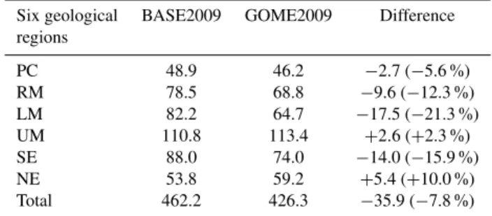
Table 1.NOxemissions inventory changes from baseline emissions inventory for August of 2009 (BASE2009) and GOME-2-adjusted emission inventory (GOME2009) over six geological regions of the US (PC: Pacific Coast, RM: Rocky Mountain, LM: Lower Middle, UM: Upper Middle, SE: Southeast, and NE: Northeast) for August 2009 (in unit of Gg N). The parentheses indicate the changes in the amounts of emissions in each geological region (in %).
Six geological BASE2009 GOME2009 Difference regions
PC 48.9 46.2 −2.7 (−5.6 %) RM 78.5 68.8 −9.6 (−12.3 %) LM 82.2 64.7 −17.5 (−21.3 %) UM 110.8 113.4 +2.6 (+2.3 %)
SE 88.0 74.0 −14.0 (−15.9 %)
NE 53.8 59.2 +5.4 (+10.0 %) Total 462.2 426.3 −35.9 (−7.8 %)
geological regions, PC and LM, and used the corresponding in-situ hourly NOxand O3data to evaluate each comparison location.
4 Results
4.1 Comparison of the NO2columns of CMAQ to those
of GOME-2
The monthly mean column retrievals for GOME-2 NO2 re-trievals and the equivalent column-integrated values of NO2 concentrations were estimated for August 2009. Gorline and Lee (2010) showed that during the three-year period of 2007 to 2009, the month of August 2009 showed the greatest pos-itive O3bias of the CMAQ-based National Air Quality Fore-cast Capability (NAQFC) modeling system. The other setup of CMAQ model showed several over- and under-estimates over CONUS during the summer in a previous study by Choi et al. (2012). The study also showed that a comparison of model-simulated and satellite-observed NO2columns exhib-ited general overestimates in concentrated population areas and underestimates in rural areas (e.g., Choi et al., 2012). In particular, the CMAQ model overestimated the NO2column over some urban areas of PC and LM (e.g., Los Angeles, CA, South Pasadena, CA, Anaheim, CA, La Habra, CA, River-side, CA, Houston, TX, Beaumont, TX, and Sulphur, LA), also found by previous studies (e.g., Martin et al., 2006; Choi et al., 2008, 2009, 2012). The following subsections will dis-cuss the impact of highly-biased NOxemissions on surface NOxand O3concentrations in the urban and outflow areas.
4.2 Satellite-adjusted NOxemissions, GOME2009
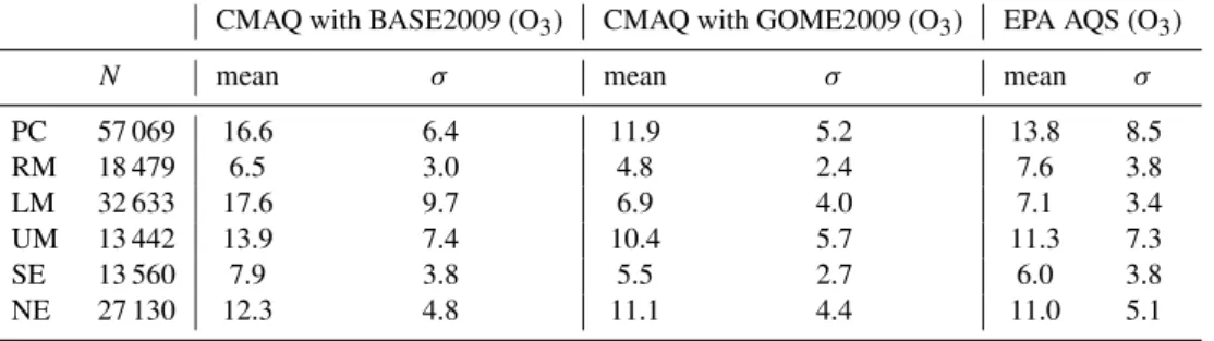
Table 2.The total number, the mean, and the standard deviation of the EPA AQS NOxobservations (in ppbv), CMAQ NOxsimulations with the base emissions, BASE2009 and CMAQ NOxsimulations with the GOME-2 adjusted emissions, GOME2009 at the EPA AQS NOx measurement sites over six geological regions of the US (PC: Pacific Coast, RM: Rocky Mountain, LM: Lower Middle, UM: Upper Middle, SE: Southeast, and NE: Northeast).
CMAQ with BASE2009 (O3) CMAQ with GOME2009 (O3) EPA AQS (O3)
N mean σ mean σ mean σ
PC 57 069 16.6 6.4 11.9 5.2 13.8 8.5
RM 18 479 6.5 3.0 4.8 2.4 7.6 3.8
LM 32 633 17.6 9.7 6.9 4.0 7.1 3.4
UM 13 442 13.9 7.4 10.4 5.7 11.3 7.3
SE 13 560 7.9 3.8 5.5 2.7 6.0 3.8
NE 27 130 12.3 4.8 11.1 4.4 11.0 5.1
were considered to adjust the emission inventories as in our previous study (e.g., Choi et al., 2012). To evaluate the NOx emissions inventory of BASE2009 over six geo-logical regions, we performed additional simulations with GOME2009 for August 2009. Again, this study focused on analyzing the relative uncertainty (instead of absolute un-certainty) of BASE2009 among the six geological regions. The sensitivity simulation, which determined the amount of NOxemissions that increased or decreased according to the ratio, found that NOx emissions decreased by about 7.8 % over the US (from 462 Gg N to 426 Gg N), and changes in the amount of emissions varied in each geological region (e.g., PC =−5.6 %, RM =−12.3 %, LM =−21.3 %, UM = +2.3 %,
SE =−15.9 %, NE = +10.0 %) (Table 1). The large
reduc-tions were shown in LM (17.5 Gg N) and SE (14.0 Gg N). The reductions may have been caused by reductions in mo-bile emissions because the consistent decrease in power plant NOxemissions was accounted for in the baseline emissions, BASE2009, but because of the limited datasets for mobile emission reductions over the contiguous US, changes in mobile sources were not (e.g., Choi et al., 2012). Interest-ingly, the opposite trend showing an increase in NO2 emis-sions appeared over NE (5.4 Gg N) in the satellite emisemis-sions, GOME2009. The trend showing an increase in GOME NO2 columns over the geological region of NE from 1996 to 2002 was found in a previous study by Richter et al. (2005). Trends showing increased NOx emissions over the region were not well simulated in the emissions modeling. Picker-ing et al. (2011) found some evidence of an increase in un-resolved NOxemissions sources in Pennsylvania, and other neighboring states. The explanation for these results remains unclear.
4.3 The impact of GOME2009 on surface NOxover six
geological regions
As we addressed above, the explanations for the large differences between the NO2 columns of CMAQ and those of GOME-2 remain unclear. However, if we as-sume that GOME-2 involves an additional constraint on the
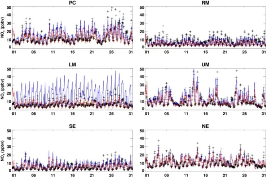
emissions inventory, we could utilize the GOME-2 NO2 columns to produce the GOME-2-adjusted emissions inven-tory, GOME2009. Then, by comparing model-simulated sur-face NOx with in-situ surface observations, we could ex-amine whether GOME2009 represents a useful constraint for a bottom-up emissions inventory. Initial comparisons of ground-level AQS NOx observations in the six geological regions (black cross) to baseline CMAQ with BASE2009 (blue) and sensitive CMAQ (red) model simulations with GOME2009 are shown in Fig. 2. The figure displays a plot of observed (black crosses) and model-simulated (blue and red solid lines, representing baseline CMAQ and CMAQ with GOME2009) NOxconcentrations at EPA AQS stations over the six geological regions in August 2009. The total number, mean, and standard deviations of AQS NOx ob-servations and corresponding CMAQ results are also esti-mated for all the measurement stations over six geologi-cal regions (Table 2). For AQS station measurements for PC, RM, LM, UM, SE, and NE regions with high correla-tion coefficients among hourly NOxconcentrations from ob-servations and CMAQ model runs (0.70 <R< 0.84), the bi-ases of the baseline CMAQ with BASE2009 are both pos-itive and negative (normalized mean bias, NMB = +19.8 %,
−13.8 %,+149.7 %,+22.5 %,+31.3 %,+11.6 %); CMAQ simulations with GOME2009 improve in terms of the abso-lute amounts of NMB (NMB =−13.7 %,−36.7 %,−1.8 %,
−7.8 %,−7.9 %,+0.7 %), except for the geological region,
RM. Analysis of these six geological regions shows three noticeable changes in the biases: reductions in NMB from
+149.7 % to −1.8 % over LM, from +31.3 % to −7.9 %
over SE, and from +19.8 % to −13.7 % over PC. We also
Fig. 2.Surface NOxconcentrations at EPA AQS stations (black crosses), corresponding CMAQ simulations with the baseline emissions, BASE2009 (blue), and CMAQ simulations including GOME-2-adjusted NOxemissions, GOME2009 (red) over six geological regions (see Fig. 1, PC: Pacific Coast, RM: Rocky Mountain, LM: Low Middle, UM: Upper Middle, SE: South East, and NE: North East) for August 2009.
Particularly over LM and PC, the pronounced large reduc-tions in simulated NOxconcentrations (in absolute amount) from the baseline to sensitivity CMAQ with GOME2009 (10.7 ppbv over LM and 4.7 ppbv over PC) (Table 2) sug-gest that NOx emissions from BASE2009 at the EPA AQS stations of geological regions LM and PC are likely to be high. The reduction in simulated NOx concentrations from the baseline CMAQ over SE was estimated to be 2.4 ppb at the EPA AQS stations, which is smaller than the reduction at the other stations over the LM and PC regions. The follow-ing sections will provide details regardfollow-ing the impact of large reductions in NOxemissions on NOxand O3concentrations in the urban areas of the LM and PC regions. We developed the new emissions inventory, GOME2009 and then evaluated the results from the CMAQ with GOME2009 by comparing them with the results of other in-situ surface observations in the urban areas and their outflow regions.
Considering all the uncertainties of the chemistry and transport in the model and remote sensing observations ad-dressed by previous studies (e.g., Richter et al., 2005; Lamsal et al., 2008; Kim et al., 2011), the relatively high simulated NOxbiases from baseline CMAQ in urban areas over LM are likely the result of over-predictions of simulated NOx emis-sions. Furthermore, the mean NOx concentrations at AQS stations over PC from high NOx emissions in urban areas such as Los Angeles are the largest (13.8 ppbv) (Table 2). In-terestingly, whereas the baseline CMAQ over-predicted NO2 columns compared to GOME-2 NO2columns in the urban
areas in southern California, the model under-predicted NO2 columns over neighboring rural regions. The explanations for the contrasting trends in the urban and rural areas are not clear, but by enhancing emissions in rural areas and reducing those in urban areas, we can at least produce similar chemical environments in terms of the amount of surface NOx concen-trations. By doing so, we can examine how changes in the chemical environments (by modifying NOxemissions) im-pact surface NOx and O3 concentrations in the urban areas and their neighboring outflow regions of PC and LM.
4.4 The impact of GOME2009 on NOxand O3
concentrations over PC
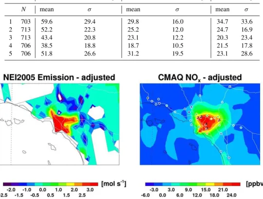
Table 3.The total number, the mean, and the standard deviation of the EPA AQS NOxobservations (in ppbv), CMAQ NOxsimulations with the baseline emissions, BASE2009 and CMAQ NOxsimulations with GOME-2 adjusted emissions, GOME2009 at the five EPA AQS NOx measurement sites (see the right panel of Fig. 3, 1: Los Angeles, 2: South Pasadena, 3: Anaheim, 4: La Habra, and 5: Riverside).
CMAQ with BASE2009 (O3) CMAQ with GOME2009 (O3) EPA AQS (O3)
N mean σ mean σ mean σ
1 703 59.6 29.4 29.8 16.0 34.7 33.6
2 713 52.2 22.3 25.2 12.0 24.7 16.9
3 713 43.4 20.8 23.1 12.2 20.3 23.4
4 706 38.5 18.8 18.7 10.5 21.5 17.8
5 706 51.8 26.6 31.2 19.5 23.1 28.6
Fig. 3. The difference between the surface NOx emissions of the baseline emissions BASE2009 and GOME-2-adjusted emissions GOME2009 (left panel, the difference is estimated only when monthly NO2 column averages are > 1015molecules cm−2from GOME-2 and CMAQ over the continent); the differences between the surface NOxconcentrations of the baseline CMAQ with BASE2009 and CMAQ with GOME2009 (right panel); and the differences between the baseline CMAQ with BASE2009 and EPA AQS observations (circles on the right panel) for the daytime (13:00–17:00 LT) of August 2009. Among the circled stations, the five marked stations (1: Los Angeles, 2: South Pasadena, 3: Anaheim, 4: La Habra, and 5: Riverside) include large discrepancies in > daytime 20 ppbv NOx(baseline CMAQ simulations – EPA AQS observations).
reductions in NOxconcentrations in the cities (> 15.0 ppbv) (Fig. 3). In addition, several increases in NOx emissions in the eastern parts of the urban cities in the satellite emis-sion, GOME2009 (see the negative values on the left panel of Fig. 3) also appear, but the impact of changes in emissions on NOxconcentrations are not evident (see the right panel of Fig. 3), likely the result of the eastward transport of signif-icantly reduced NOx air in urban cities (Fig. 3). In conclu-sion, the large changes in surface NOxemissions mitigated the large discrepancies in CMAQ simulated NOx concentra-tions (see the circles on the right panel of Fig. 3), compared to corresponding EPA AQS observations (Fig. 3).
To evaluate how the GOME2009 emissions inventory af-fects the NOxconcentrations at five station grids (including the discrepancies of > 20 ppbv NOx concentrations during the daytime (13:00–17:00 LT), compared to the correspond-ing EPA AQS observations), we estimate three sets of NOx concentrations from CMAQ simulations with BASE2009,
CMAQ simulations with GOME2009, EPA AQS observa-tions (Table 3). Estimates of the mean values of the surface NOx concentrations at the AQS sites were 34.7, 24.7, 20.3, 21.5, and 23.1 ppbv at the five station grids (1: Los Ange-les, 2: South Pasadena, 3: Anaheim, 4: La Habra, and 5: Riverside) (Table 3). Estimated surface NOxconcentrations of the baseline CMAQ model were 59.6, 52.2, 43.4, 38.5, and 51.8 ppbv at the grids. The corresponding estimates from CMAQ with GOME2009 were 29.8, 25.2, 23.1, 18.7, and 31.2 ppbv, which were similar to those of EPA AQS observa-tions.
Statistically, the baseline CMAQ model significantly over-predicted surface NOxconcentrations at the five station grids by+71.8,+111.3,+113.8,+79.1, and+124.2 % (Table 3).
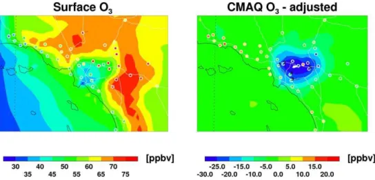
Fig. 4.Surface O3concentrations from the baseline CMAQ with baseline emissions, BASE2009 (left panel), and EPA AQS measurements (circles on the left panel), the difference between the surface O3of the baseline CMAQ with BASE2009 and CMAQ with GOME-2-adjusted NOxemissions GOME2009 (right panel) and the difference between the surface O3of the baseline CMAQ with BASE2009 and EPA AQS (circles on the right panel, baseline CMAQ simulations – EPA AQS observations) for the daytime (13:00–17:00 LT) in August 2009.
discrepancies in NOxconcentrations at the five station grids (Fig. 4).
Because of the complexity of O3 production, changes in surface O3 following changes in NOx emissions are more difficult to understand. Large reductions in NOxemissions in urban cities such as Los Angeles result in large increases in daytime O3(13:00–17:00 LT) in the areas and the downwind from the urban cities is caused by westerly see breezes during the daytime in the summer. As Los Angeles is a typical NOx-saturated regime area, the large reductions in NOxemissions resulted in large increases in surface O3 concentrations in the urban city and its neighboring areas (see the right panel of Fig. 5). Interestingly, the CMAQ with BASE2009 under-predicted surface O3 in and near Los Angeles and South Pasadena and their outflow areas, including Riverside (up to 30 ppbv) (see the circles of the right panel of Fig. 5). Thus, the large increases in simulated surface O3following signifi-cant reductions in NOxemissions in Los Angeles, Pasadena, and Anaheim resulted in trends of pre-existing simulated under-prediction to those of over-prediction in the areas (see the right panel of Fig. 5).
Large reductions in NOxemissions resulted in reductions in NOxconcentrations and increases in O3concentrations in the urban cities (Figs. 4 and 5), which is a typical trend shown in NOx-saturated regime. For example, the baseline CMAQ model under-predicted surface O3concentrations by−22.7,
−27.1,−23.4,−13.1 and−31.3 % at the five station grids, and the large reductions in NOxemissions increased surface O3concentrations, which resulted in overestimation of the surface O3predictions of+37.6,+31.3,+19.5,+38.1, and +9.6 % (Table 4). In other words, the large reduction in NOx
emissions introduced the over-prediction of surface O3 con-centrations in CMAQ with GOME2009 (Fig. 6).
We also investigated how O3 concentrations vary dur-ing the daytime (13:00–17:00 LT) from baseline CMAQ to CMAQ with GOME2009. Similarly, during the daytime, the CMAQ model under-predicted surface O3concentrations by
−12.9,−29.0,−24.8,−20.9, and−27.2 % at the five station
grids, and large reductions in NOxemissions significantly in-creased surface O3concentrations; thus, the under-prediction patterns became over-prediction patterns of +25.4, +12.0,
+11.5,+19.6, and +9.2 % at the five grids (see the paren-theses in Table 4). During the daytime, except for the station in Los Angeles, the large biases of surface O3at the stations in South Pasadena, Anaheim, La Habra, and Riverside de-creased as a result of reductions in NOxemissions. The large NOx reductions mitigated the large discrepancies between the NOx concentrations of the baseline CMAQ and those of corresponding AQS observations and enhanced simulated surface O3concentrations, but the increases in O3 concentra-tions were extreme, likely stemming from the high sensitivity of surface O3to changes in NOxemissions. Interestingly, the low biases of baseline CMAQ during the daytime (13:00– 17:00 LT) decreased in a more similar manner than those of the baseline CMAQ during the whole day, even with the large increase in nighttime O3 caused by a reduction in surface NOx emissions (Fig. 6). Explanations for this phenomenon remain unclear, probably because the CMAQ model repre-sents the urban areas as extreme NOx-saturated regime (in-stead of normal NOx-saturated areas or mixed areas, shown in Fig. 3 of the previous study by Choi et al., 2012), likely due to the overestimated NOxemissions.
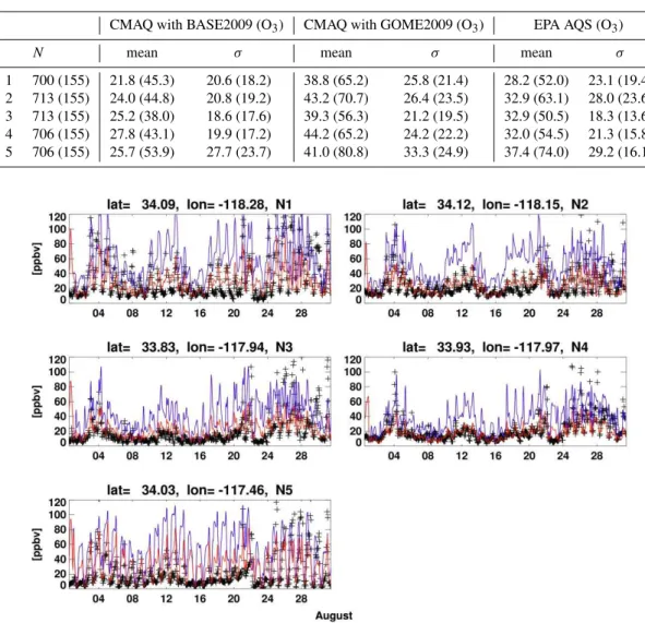
Table 4.The total number, the mean, and the standard deviation of the EPA AQS O3observations (in ppbv), CMAQ O3simulations with the baseline emissions, BASE2009 and CMAQ O3simulations with GOME-2 adjusted emissions, GOME2009 at the five EPA AQS O3 measurement sites (see the right panel of Fig. 3, 1: Los Angeles, 2: South Pasadena, 3: Anaheim, 4: La Habra, and 5: Riverside). The parentheses indicate the corresponding data during the daytime (13:00–17:00 LT).
CMAQ with BASE2009 (O3) CMAQ with GOME2009 (O3) EPA AQS (O3)
N mean σ mean σ mean σ
1 700 (155) 21.8 (45.3) 20.6 (18.2) 38.8 (65.2) 25.8 (21.4) 28.2 (52.0) 23.1 (19.4) 2 713 (155) 24.0 (44.8) 20.8 (19.2) 43.2 (70.7) 26.4 (23.5) 32.9 (63.1) 28.0 (23.6) 3 713 (155) 25.2 (38.0) 18.6 (17.6) 39.3 (56.3) 21.2 (19.5) 32.9 (50.5) 18.3 (13.6) 4 706 (155) 27.8 (43.1) 19.9 (17.2) 44.2 (65.2) 24.2 (22.2) 32.0 (54.5) 21.3 (15.8) 5 706 (155) 25.7 (53.9) 27.7 (23.7) 41.0 (80.8) 33.3 (24.9) 37.4 (74.0) 29.2 (16.1)
Fig. 5.Surface NOxconcentrations at EPA AQS stations (black crosses), corresponding baseline CMAQ simulations with baseline emissions, BASE2009 (blue), and CMAQ simulations with GOME-2-adjusted NOxemissions, GOME2009 (red) at the five station grids (see the right panel of Fig. 3, 1: Los Angeles, 2: South Pasadena, 3: Anaheim, 4: La Habra, and 5: Riverside) in August 2009.
SCIAMACHY)-observed NO2 columns are approximately twice as small as the corresponding WRF-Chem-simulated NO2 columns in the urban areas along the US West Coast. They suggested that these differences were caused by over-estimated NOx emissions in the areas from an updated NEI1999 in their study. Again, in this study, unlike in previ-ous studies, we reveal that satellite-adjusted emissions mit-igated simulated NOx and daytime O3 discrepancies com-pared to the corresponding observations.
4.5 The impact of GOME2009 on NOxand O3
concentrations over LM
Fig. 6.Surface O3concentrations at EPA AQS stations (black crosses), corresponding baseline CMAQ simulations with baseline emissions, BASE2009 (blue), and CMAQ simulations with GOME-2-adjusted NOxemissions, GOME2009 (red) at the five station grids (see the right panel of Fig. 3, 1: Los Angeles, 2: South Pasadena, 3: Anaheim, 4: La Habra, and 5: Riverside) in August 2009.
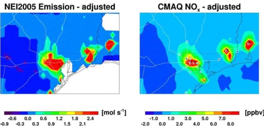
Fig. 7.The differences between surface NOxemissions of baseline emissions, BASE2009 and GOME-2-adjusted emissions, GOME2009 (left panel, the difference is estimated only when monthly NO2column averages are > 1015molecules cm−2from GOME-2 and CMAQ over the continent); the differences between the surface NOxconcentrations of the baseline CMAQ with BASE2009 and CMAQ with GOME2009 (right panel); and the differences between surface NOxconcentrations of the baseline CMAQ with BASE2009 and EPA AQS observations (circles on the right panel) for the daytime (13:00–17:00 LT) of August of 2009. Among the circled stations, the four marked stations (1: Houston A, 2: Houston B, 3: Beaumont, and 4: Sulphur) include the large discrepancies of > daytime 10 ppbv NOx(baseline CMAQ simulations – EPA AQS observations).
in the urban areas resulted in reductions in NOx concentra-tions in the cities (> 8.0 ppbv) (Fig. 7). In addition, some in-creases in NOxemissions over the western parts of Houston
resulted in increases in NOxconcentrations (> 2.0 ppbv) dur-ing the daytime (Fig. 7).
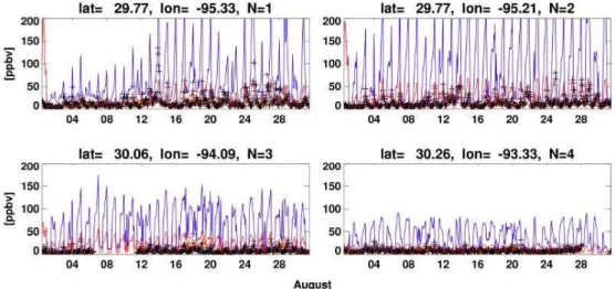
Fig. 8.Surface NOxconcentrations at EPA AQS stations (black crosses), corresponding baseline CMAQ simulations with baseline emissions, BASE2009 (blue), and CMAQ simulations with GOME-2-adjusted NOxemissions, GOME2009 (red) at the four station grids (see the right panel of Fig. 7, 1: Houston A, 2: Houston B, 3: Beaumont, and 4: Sulphur) in August 2009.
Fig. 9.The differences between the O3concentrations from a baseline CMAQ with baseline emissions, BASE2009 (left panel) and EPA AQS measurements (circles on the left panel); the differences between surface O3of the baseline CMAQ with BASE2009 and CMAQ with GOME-2-adjusted NOxemissions, GOME2009 (right panel); and the differences between surface O3of the baseline CMAQ with BASE2009 and EPA AQS (circles on the right panel, baseline CMAQ simulations – EPA AQS observations) for the daytime (13:00–17:00 LT) of August of 2009.
model, we examine four station grids for the urban areas (Fig. 8). We chose the four grids because they exhibited large differences between the baseline CMAQ simulated and AQS observed NOx concentrations of > 10 ppbv during the daytime (13:00–17:00 LT) (see the right panel of Fig. 7). For more details, we compared the surface NOxconcentrations from baseline CMAQ and CMAQ with GOME2009 to the corresponding in-situ observations at four different station grids (Fig. 8). Our analysis showed that the baseline CMAQ model over-predicted surface NOx concentrations by +288.0, +464.2, +683.1, and +402.5 % at the four station grids (Table 5 and Fig. 8). Interestingly, from the baseline CMAQ, the diurnal differences in the surface NOx
concentrations in the urban areas of LM were significantly larger than those in the urban areas of PC. The baseline CMAQ significantly overestimated the surface NOx, partic-ularly during the nighttime in the urban areas of LM, partly because of the underestimated PBL heights over the Gulf Coast areas, as Eder et al. (2009) previously found.
The large reductions in NOx emissions led to signifi-cant reductions in NOx concentrations and thus mitigated the discrepancies between simulated NOxconcentrations of baseline CMAQ and corresponding AQS observations, and those of CMAQ with GOME2009 became as+15.8,+65.5,
Fig. 10.Surface O3concentrations at EPA AQS stations (black crosses), corresponding baseline CMAQ simulations with baseline emissions, BASE2009 (blue), and CMAQ simulations with GOME-2-adjusted NOxemissions, GOME2009 (red) at the four station grids (see the right panel of Fig. 7, 1: Houston A, 2: Houston B, 3: Beaumont, and 4: Sulphur) in August 2009.
Table 5.The number, the mean, and the standard deviation of the EPA AQS NOxobservations (in ppbv), CMAQ NOxsimulations with the baseline emissions, BASE2009 and CMAQ NOxsimulations with GOME-2 adjusted emissions, GOME2009 at the four different EPA AQS measurement sites (see the right panel of Fig. 7, 1: Houston A, 2: Houston B, 3: Beaumont, and 4: Sulphur).
CMAQ with BASE2009 (O3) CMAQ with GOME2009 (O3) EPA AQS (O3)
N mean σ mean σ mean σ
1 727 61.3 51.2 18.3 21.6 15.8 13.5
2 732 83.5 70.4 24.5 24.7 14.8 11.2
3 615 60.3 39.4 21.0 14.3 7.7 6.0
4 643 39.7 22.8 11.6 6.6 7.9 4.1
at the four urban areas, but the overestimates of the baseline CMAQ model significantly decreased (Fig. 8).
The large reductions in NOx emissions in the urban ar-eas of LM region generally resulted in large reductions in daytime O3(13:00–17:00 LT) over regions downwind from the urban cities (e.g., over forested regions represented by an extreme NOx-sensitive regime) because of the distinctive southerly or southeasterly sea breezes during the daytime in the summer (see the right panel of Fig. 9). In another words, in the forested areas over the region downwind from Houston and Beaumont, TX and Sulphur, LA (e.g., Sam Houston Na-tional Forest and Devy Crockell NaNa-tional Forest), monthly-averaged daytime O3concentrations significantly decreased by > 6 ppbv as a result of reductions in NOxemissions in the urban cities (see the right panel of Fig. 9). During the sum-mertime, dominant sea breezes from the ocean blow into the area following a large reduction in NOxemissions in the cen-tral cities during the daytime, resulting in large O3reductions over the NOx-sensitive regime (Fig. 9).
Large reductions in NOxemissions resulted in several in-creases in surface O3concentrations in the core cities (e.g., Houston and Sulphur) (Table 6). For example, during the
daytime (13:00–17:00 LT), the baseline CMAQ originally over-predicted surface O3 (about 8 ppbv) in Houston and (about 2 ppb) Sulphur (see the parentheses of Table 6). Thus, the large increases in simulated surface O3following the sig-nificant reductions in NOxemissions in central Houston and Sulphur exacerbated pre-existing simulated over-prediction trends in the areas (Table 6).
This study showed that overestimates of simulated surface O3 in the urban centers or industrial areas were relatively smaller than those of the simulated O3 in the other areas of Houston (see the left panel of Fig. 9) likely the result of the limitation of the CMAQ model, that is, its inability to capture temporary high-peak O3phenomena in central or in-dustrial areas. The monthly-averaged surface O3 concentra-tion plot does not fully represent specific-surface O3peaks near the Houston Ship Channel as Daum et al. (2003) and Xiao et al. (2010) showed in their studies. Thus, the ratio of VOC/NOxas a proxy of the chemical environment needs further investigation.
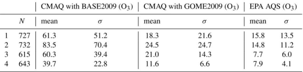
Table 6.The number, the mean, and the standard deviation of the EPA AQS O3observations, CMAQ O3simulations with the baseline emissions, BASE2009 and CMAQ O3simulations with GOME-2 adjusted emissions, GOME2009 at the four EPA AQS O3measurement sites (see the right panel of Fig. 7, 1: Houston A, 2: Houston B, 3: Beaumont, and 4: Sulphur). The parentheses indicate the corresponding data during the daytime (13:00–17:00 LT).
CMAQ with BASE2009 (O3) CMAQ with GOME2009 (O3) EPA AQS (O3)
N mean σ Mean σ mean σ
1 738 (155) 19.4 (46.1) 20.1 (16.1) 32.3 (53.0) 18.4 (11.7) 20.9 (38.1) 17.1 (18.4) 2 740 (155) 18.3 (48.7) 22.4 (16.3) 26.9 (51.2) 20.8 (10.6) 22.7 (41.3) 18.1 (19.2) 3 737 (154) 16.1 (38.9) 20.1 (16.8) 23.1 (41.4) 17.2 (10.3) 25.4 (40.1) 18.3 (17.9) 4 730 (155) 15.8 (35.6) 18.1 (16.3) 26.8 (40.2) 13.7 (10.4) 19.4 (33.3) 15.2 (13.2)
CMAQ model revealed negative biases of simulated sur-face O3concentrations compared to corresponding observa-tions (Fig. 10). At the four marked station grids, the baseline CMAQ model under-predicted O3 concentrations by −7.2, −19.4, −36.6, and −18.6 % (see the blue colored line of
Fig. 10). The large reductions in NOxemissions (Fig. 7) gen-erally increased surface O3concentrations and the underpre-diction trends of CMAQ became weaker or changed to over-prediction trends. For example, at the four station grids, the estimates of the biases of the CMAQ model with GOME2009 were+55.5,+18.5,−9.1 and+38.1 % (see the red colored line of Fig. 10).
During the daytime (13:00–17:00 LT), estimates of the bi-ases of the baseline CMAQ were+21.0,+17.9,−3.0, and
+6.9 %, and emissions of the biases of the CMAQ with GOME2009 changed to+39.1,+24.0,+3.2, and+20.7 % at
the four station grids in the urban areas (see the parentheses of Table 6). The baseline CMAQ originally overestimated or slightly underestimated surface O3concentrations in the ur-ban areas during the daytime, and the large reduction in the surface NOxemissions resulted in the large increase in simu-lated O3concentrations in the areas. Thus, the increased sur-face O3concentrations from the model with GOME2009 in-creased trends of overestimation of the baseline CMAQ (Ta-ble 6).
Consistent with the results of a previous study by Choi et al. (2012), the results of this study show that CMAQ recognizes the central urban areas of LM as extreme NOx-saturated regime areas (by the overestimates of NOx emis-sions). The high-biased NOx concentrations in the urban cores might enhance surface O3more over the regions down-wind from the urban cities (particularly in the forecasted ar-eas in northar-eastern Houston) (Fig. 9). Because of the op-posing chemical characteristics of these two areas regard-ing O3 sensitivity (e.g., urban cores: NOx-saturated area and forests: NOx-sensitive area) to changes in NOx emis-sions/concentrations, designing an efficient O3control strat-egy for both areas poses a challenge. Whereas Li et al. (2007) showed the impact of the reduction in biogenic VOC emis-sions in forested areas in northeastern Houston on surface O3 in the urban core of Houston, this study showed the impact
of the reduction in surface NOxemissions in urban cores on surface O3over the outflow regions from Houston (Fig. 9).
The explanation for preexisting high O3biases (> 6 ppbv) in CMAQ in Houston (see the circles on the right panel of Fig. 9) remains unclear. However, the over-prediction of NOx emissions in Houston, shown in Fig. 7, is likely a major cause of the over-predicted NOxconcentrations, and the large NOxemissions reductions significantly mitigate the discrep-ancies of the baseline CMAQ compared to the correspond-ing AQS observations (see the right panel of Fig. 7), but the overestimated NOxemissions cannot solely explain the over-prediction of the surface O3in the area. The large NOx reduc-tions in GOME2009 mitigated the high O3 biases over the outflow region of and around the urban cities, but they exac-erbated the O3high biases of the baseline CMAQ in the core of Houston and Sulphur (Table 6). In Beaumont, the large NOxreductions increased the simulated surface O3 concen-trations, which resulted in mitigating low O3 biases of the baseline CMAQ in urban areas such as Los Angeles.
5 Conclusion and discussion
To evaluate the baseline emissions inventory, BASE2009, we analyzed simulation results from CMAQ over six geologi-cal regions over the CONUS. We obtained NOx emissions inventory, GOME2009, from BASE2009 over the CONUS using ratios of CMAQ to GOME-2 NO2column density. We found large reductions in NOxconcentrations in CMAQ with GOME2009, at EPA AQS stations over LM, SE and PC (i.e.,
+149.7 to −1.8 % for LM and+19.8 to−13.7 % for PC),
which resulted from large reductions in NOxemissions over the regions. The GOME2009 significantly reduced the biases of the NOxconcentrations in the urban areas of the LM and PC regions of CMAQ simulations and AQS observations, re-sulting in the mitigation of the simulated discrepancies of baseline CMAQ.
The results of this study indicated that NOx emissions from BASE2009 in the urban areas of LM (e.g., Houston, Beaumont, and Sulphur) and PC regions (e.g., Los Ange-les, South Pasadena, Anaheim, La Habra, and Riverside) are abnormally high, indicating large relative uncertainty of BASE2009 NOx emissions. The analysis of simulation re-sults from global/regional CTMs and climate models must account for these high NOxbiases in the urban areas of LM and PC. For example, significant reductions in NOx emis-sions led to large reductions in model simulations of surface NOxat AQS stations in the urban areas of LM and PC. In par-ticular, in the urban areas of LM, the largest discrepancies in simulated surface NOxconcentrations are significantly mit-igated in the areas, compared to corresponding observations from AQS. These results suggest that remote-sensing data could be another useful constraint of the bottom-up emis-sions inventory. Furthermore, changes in NOx emissions in the urban areas of LM and PC in GOME2009 compared to those in BASE2009 are useful for not only updating the emis-sions inventory but also mitigating the discrepancies in the chemical environment such as NOxconcentrations.
In general, while the large reductions in NOxemissions in GOME2009 mitigated the discrepancies in the simulated O3 concentrations in the urban areas of PC region (e.g., South Pasadena, La Habra and Riverside) and the LM region (e.g., Beaumont), the large reductions in emissions exacerbated over-predictions of pre-existing biased surface O3in urban core areas in Houston and Sulphur of LM in the baseline CMAQ resulting from the increase in surface O3 from re-ductions in NOx emissions. However, the large reductions in NOxemissions mitigate the high O3biases over outflow region or around the main core of Houston (see the right panel of Fig. 9). Again, reductions in the over-predictions of pre-existing simulated large O3 in the urban core cities of LM in baseline CMAQ did not occur as a result of reduc-tions in the high over-predicreduc-tions of NOxemissions except in Beaumont; thus, to explain simulated high O3bias over the southern US from CTMs, shown in previous studies (e.g., McKeen et al., 2009; Kim et al., 2011), we need to divide
urban areas into urban core cities and near or outflow region of the urban core and test two areas separately. In addition to NOxconcentrations, the emissions of VOCs over the LM and PC regions require further investigation. In future research, we will introduce another remote-sensing product such as HCHO columns as a proxy for VOC measurements. In ad-dition, we will divide high O3-biased regions into chemical regimes, which might prove useful for determining the cause of high O3biases.
As Kim et al. (2011) stated, if we have more VOC emis-sions and fewer NOx emissions in the industrial areas of Houston, we might simulate similar chemical environments in the areas. However, they also showed that simulated O3 concentrations still exhibit large discrepancies compared to in-situ observed O3concentrations. In a future study, we will first modify the chemical environment (both NOxand VOC) in the areas, which might alter the chemical characteristics of an extreme NOx-saturated regime region to those of a less NOx-saturated regime region or a mixed regime region in industrial and urban areas. For example, as we addressed above, as a proxy for VOC emissions, we will also evaluate simulated HCHO column densities in the model and compare them to remote-sensing HCHO columns. After performing this evaluation, we can evaluate the ratio of the simulated HCHO/NO2columns (as a proxy for the chemical environ-ment, VOC/NOx) to those of corresponding remote-sensing observations. Of course, one challenge of this task is how we consider the uncertainty of remote sensing, such as that stemming from the products of HCHO columns.
This study also found that during the summertime, the sig-nificant reduction of NOxemissions in urban core cities re-sulted in an increase in surface O3 in the urban areas (e.g., Los Angeles, South Pasadena, Anaheim, La Habra, River-side, Houston, Beaumont, and Sulphur), but resulted in large reductions in surface O3 in forested areas or outflow re-gions over northeastern or northern rere-gions downwind from urban cities (e.g., Houston and Beaumont). These large re-ductions are not clearly shown in outflow regions of ur-ban cities in southern California (e.g., near Los Angeles) likely because of lower VOC concentrations in the outflow regions. In other words, while the NOx-saturated regime be-comes NOx-sensitive regime as the location moves from ur-ban cities of Houston and Beaumont of LM to their out-flow rural or forested regions, the characteristics of the NOx-saturated regime of the urban area of Los Angeles remain stable, as do those of the outflow region from the urban city because of limited VOC sources. In a future study, we plan to investigate how quickly the chemical regime from urban areas to outflow areas changes, the purpose of which is to design an optimal O3pollution control strategy for each ur-ban area.
some of remaining issues. First, the assumption that remote-sensing NO2 columns are closer to actual true values com-pared with model-simulated NO2columns was not perfectly met by the results. Thus, ideally, in order to get accu-rate emission inventories, we need to estimate uncertainties of remote-sensing NO2 column and model simulated NO2 column/NOx emission inventories and use the uncertainties for the application of data assimilation approach (e.g., Nape-lenok et al., 2008; Chai et al., 2009; Zhao and Wang, 2009). Second, emissions were adjusted using morning time satel-lite NO2column data (e.g., GOME-2) and the resulting emis-sion inventory could miss its diurnal cycle. In a following study, we will adjust the diurnal cycles of emissions using two different remote-sensing data from GOME-2 (morning time) and OMI (afternoon). Some other uncertainties regard-ing the use of NO2columns as a proxy for NOx concentra-tions/emissions over the surface were described in detail in the previous study (e.g., Choi et al., 2012).
More interestingly, the high simulated NOx biases are still shown in the comparison of the NOx concentrations from CMAQ including NEI2008 from Air Quality Forecast-ing system at UH (AQF-UH) and the correspondForecast-ing obser-vations from the CAMS sites over southeastern Texas for the DISCOVER-AQ Houston campaign (September of 2013) (Appendix A), but they are not shown to be significant as much as in those of CMAQ including the modified NEI2005 in this study. The detailed study needs to be followed to ex-amine how high biases of NOxemissions found in this study are changed in the modeling study with NEI2008 using same resolution and same time simulations.
Supplementary material related to this article is available online at http://www.atmos-chem-phys.net/14/ 675/2014/acp-14-675-2014-supplement.pdf.
Acknowledgements. This work is dedicated to the memory of Dr. Daewon Byun (1956–2011), whose pursuit of scientific excellence as a developer of the CMAQ model continues to inspire us. This study is partially supported by the Texas Air Research Center (TARC) funding (413UHH0144A). I thank Daniel Tong and Hyuncheol Kim for the preparation of the emissions data, Pius Lee and other NOAA ARL and NWS group members, Beata Czader, Xiangshang Li and Mark Estes for the preparation of the comparisons of the AQF-UH and CAMS site data, and Barry Lefer, Robert Talbot, Xun Jiang, and atmospheric science graduate students at the University of Houston for their useful comments. I also acknowledge the free use of tropospheric NO2column data from the GOME-2 sensor from www.temis.nl.
Edited by: C. H. Song
References
Beirle, S., Platt, U., Wenig, M., and Wagner, T.: Weekly cycle of NO2 by GOME measurements: a signature of anthropogenic sources, Atmos. Chem. Phys., 3, 2225–2232, doi:10.5194/acp-3-2225-2003, 2003.
Brioude, J., Kim, W., Angevine, W. M., Frost, G. J., Lee, S.-H., McKeen, S. A., Trainer, M., Fehsenfeld, F.C., Holloway, J. S., Ryerson, T. B., Williams, E. J., Petron, G., and Fast, J. D.: Top-down estimate of anthropogenic emission inventories and their interannual variability in Houston using a mesoscale inverse modeling technique, J. Geophys. Res., 116, D20305, doi:10.1029/2011JD016215, 2011.
Chai, T., Carmichael, G. R., Tang, Y., Sandu, A., Heckel, A., Richter, A., and Burrows, J. P.: Regional NOxemission inversion through a four-dimensional variational approach using SCIA-MACHY tropospheric NO2column observations, Atmos. Env-iron., 43, 5046–5055, 2009.
Choi, Y., Wang, Y., Zeng, T., Cunnold, D., Yang, E., Martin, R., Chance, K., Thouret, V., and Edgerton, E: Spring to summer northward migration of high O3over the western North Atlantic, Geophys. Res. Lett, 35, L04818, doi:10.1029/2007GL032276, 2008.
Choi, Y., Kim, J., Eldering, A., Osterman, G., Yung, Y. L., Gu, Y., and Liou, K. N.: Lightning and anthropogenic NOxsources over the United States and the western North Atlantic Ocean: Impact on OLR and radiative effects, Geophys. Res. Lett, 36, L17806, doi:10.1029/2009GL039381, 2009.
Choi, Y., Kim, H., Tong, D., and Lee, P.: Summertime weekly cycles of observed and modeled NOxand O3concentrations as a func-tion of satellite-derived ozone producfunc-tion sensitivity and land use types over the Continental United States, Atmos. Chem. Phys., 12, 6291–5307, doi:10.5194/acp-12-6291-2012, 2012.
Daum, P. H., Kleinman, L. I., Springston, S. R., Nunnermacker, L.J., Lee, Y.-N., Weinstein-Lloyd, J., Zheng, J., and Berkowtiz, C. M.: A comparative study of O3formation in the Houston urban and industrial plumes during the 2000 Texas Air Quality Study, J. Geophys. Res., 108, 4715, doi:10.1029/2003JD003552, 2003. Eder, B., Kang, D., Mathur, R., Pleim, J., Yu, S., Otte, T., and
Pouliot, G.: A performance evaluation of the National Air Qual-ity Forecast CapabilQual-ity for the summer of 2007, Atmos. Environ., 43, 2312–2320, 2009.
Foley, K. M., Roselle, S. J., Appel, K. W., Bhave, P. V., Pleim, J. E., Otte, T. L., Mathur, R., Sarwar, G., Young, J. O., Gilliam, R. C., Nolte, C. G., Kelly, J. T., Gilliland, A. B., and Bash, J. O.: Incremental testing of the Community Multiscale Air Quality (CMAQ) modeling system version 4.7, Geosci. Model Dev., 3, 205–226, doi:10.5194/gmd-3-205-2010, 2010.
Gorline, J. and Lee, P.: Performance of NOAA-EPA Air Quality Prediction, 2007–2009 CMAS conference 2010, www.cmascenter.org/conference/2009/abstracts/gorline_ performance_noaa-epa_2009.pdf, 2010.
Han, K. M., Lee, C. K., Lee, J., Kim, J., and Song, C. H.: A com-parison study between model-predicted and OMI-retrieved tro-pospheric NO2columns over the Korean peninsula, Atmos. En-viron., 45, 2962–2971, 2010.
the UAM-V photochemical grid model applied to the July 1995 OTAG domain, Atmos. Environ., 35, 891–903, 2003.
Henderson, B. H., Jeffries, H. E., Kim, B. U., and Vizuete, W. G.: The influence of model resolution on ozone in industrial volatile organic compound plumes, J. Air Waste Manage. Assoc., 60, 1105–1117, 2010.
Houyoux, M. R., Vukovich, J. M., Coats, C. J., Wheeler, N. J. M., and Kasibhatla, P. S.: Emission inventory development and pro-cessing for the Seasonal Model for Regional Air Quality (SM-RAQ) project, J. Geophy. Res., 105, 9079–9090, 2000.
Hudman, R. C., Jacob, D. J., Turquety, S., Leibensperger, E. M., Murray, L.T., Wu, S., Gilliland, A. B., Avery, M., Bertram, T. H., Brune, W., Cohen, R. C., Dibb, J. E., Flocke, F. M., Fried, A., Holloway, J., Neuman, J. A., Orville, R., Perring, A., Ren, X., Sachse, G. W., Singh, H. B., Swanson, A., and Wooldridge, P. J.: Surface and lightning sources of nitrogen oxides over the United States: Magnitudes, chemical evolution, and outflow, J. Geophys. Res., 112, D12S05, doi:10.1029/2006JD007912, 2007. Kaynak, B., Hu, Y., Martin, R. V., Sioris, C. E., and Russell, A. G.:
Comparison of weekly cycle of NO2satellite retrievals and NOx emission inventories for the continental U.S., J. Geophys. Res., 114, D05302, doi:10.1029/2008JD010714, 2009.
Kim, S. W., Heckel, A., McKeen, S. A., Frost, G. J., Hsie, E.-Y., Trainer, M. K., Richter, A., Burrows, J. P., Peckham, S. E., and Grell, G. A.: Satellite observed U.S. power plant NOxemission reductions and their impact on air quality, Geophys. Res. Lett., 33, 122812, doi:10.1029/2006GL027749, 2006.
Kim, S. W., Heckel, A., Frost, G. J., Richter, A., Gleason, J., Bur-rows, J. P., McKeen, S., Hsie, E.-Y., Granier, C., and Trainer, M.: NO2columns in the western United States observed from space and simulated by a regional chemistry model and their im-plications for NOxemissions, J. Geophys. Res., 114, D11301, doi:10.1029/2008JD011343, 2009.
Kim, S. W., McKeen, S. A., Frost, G. J., Lee, S.-H., Trainer, M., Richter, A., Angevine, W. M., Atlas, E., Bianco, L., Boersma, K. F., Brioude, J., Burrows, J. P., de Gouw, J., Fried, A., Glea-son, J., Hilboll, A., Mellqvist, J., Peischl, J., Richeter, D., Rivera, C., Ryerson, T., Hekkert, S., Walega, J., Warneke, C., Weib-ring, P., and Williams, E.: Evaluation of NOxand highly reac-tive VOC emission inventories in Texas and their implications for ozone plume simulations during the Texas Air Quality Study 2006, Atmos. Chem. Phys., 11, 11361–11386, doi:10.5194/acp-11-11361-2011, 2011.
Lamsal, L. N., Martin, R. V., van Donkelaar, A., Steinbacher, M., Celarier, E. A., Bucesela, E., Dunlea, E. J., and Pinto, J. P.: Ground-level nitrogen dioxide concentrations inferred from the satellite-borne Ozone Monitoring Instrument, J. Geophys. Res., 113, D16308, doi:10.1029/2007JD009235, 2008.
Lamsal, L. N., Martin, R. V., Padmanabhan, A., van Donke-laar, A., Zhang, Q., Sioris, C. E., Chance, K., Kurosu, T. P., and Newchurch, M. J.: Application of satellite ob-servations for timely updates to global anthropogenic NOx emission inventories, Geophys. Res. Lett., 38, L05810, doi:10.1029/2010GL046476, 2011.
Li, G., Zhang, R., Fan, J., and Tie, X.: Impacts of biogenic emis-sions on photochemical ozone production in Houston, Texas, J. Geophys. Res., 112, D10309, doi:10.1029/2006JD007924, 2007.
Martin, R. V., Jacob, D. J., Chance, K., Kurosu, T. P., Palmer, P. I., and Evans, M. J.: Global inventory of nitrogen oxide emis-sions constrained by space-based observations of NO2columns, J. Geophys. Res., 108, 4537, doi:10.1029/2003JD003453, 2003. Martin, R. V., Sioris, C. E., Chance, K., Ryerson, T. B., Bertram, T. H., Wooldridge, P. J., Cohen, R. C., Neuman, J. A., Swanson, A., and Flocke, F. M.: Evaluation of space-based constraints on global nitrogen oxide emissions with regional aircraft measure-ments over and downwind of eastern North America, J. Geophys. Res., 111, D15308, doi:10.1029/2005JD006680, 2006.
McKeen, S., Grell, G., Peckham, S., Wilczak, J., and Djalaova, I.: An evaluation of real-time air quality forecasts and their urban emissions over eastern Texas during the summer of 2006 Sec-ond Texas Air Quality Study field study, J. Geophys. Res., 114, D00F11, doi:10.1029/2008JD011697, 2009.
Napelenok, S. L., Pinder, R. W., Gilliland, A. B., and Martin, R. V.: A method for evaluating spatially-resolved NOxemissions using Kalman filter inversion, direct sensitivities, and space-based NO2 observations, Atmos. Chem. Phys., 8, 5603–5614, doi:10.5194/acp-8-5603-2008, 2008.
Pickering, K., Prados, A., and Napelenok, S.: Monitoring Air Qual-ity Changes in Regions Influenced by Major Point Sources over the Eastern and Central United States Using Aura/OMI NO2, 2011 CMAS conference, 2011.
Richter, A., Burrows, J. P., Nub, H., Granier, C., and Niemeier, U.: Increase in tropospheric nitrogen dioxide over China observed from space, Nature, 437, 129–132, 2005.
Russell, A. R., Valin, L. C., Bucsela, E. J., Wenig, M. O., and Cohen, R. C.: Space-based Constraints on Spatial and Temporal Patterns of NOxEmissions in California, 2005–2008, Environ. Sci. Tech-nol., 44, 3608–3615, 2010.
Xiao, X., Cohen, D. S., Byun, D. W., and Ngan, F.: Highly non-linear ozone formation in the Houston region and implications for emission controls, Environ. Sci. Technol., 115, D23309, doi:10.1029/2010JD014435, 2010.
Yang, Q., Wang, Y., Zhao, C., Liu, Z., Gustafson, W. I., and Shao, M.: NOxemission reduction and its effects on ozone during the 2008 Olympic Games, Environ. Sci. Technol., 45, 6404–64210, 2011.
Yoshida, Y., Duncan, B. N., Retscher, C., Pickering, K. E., Celarier, E. A., Joiner, J., Boersma, K. F., and Weefkind, J. P.: The impact of the 2005 Gulf Hurricanes on pollution emissions as inferred from Ozone Monitoring Instrument (OMI) nitrogen dioxide, At-mos. Environ., 44, 1443–1448, 2010.
Zhao, C. and Wang, Y.: Assimilated inversion of NOxemissions over East Asia using OMI NO2column measurements, Geophys. Res. Lett., 36, L06805, doi:10.1029/2008GL037123, 2009. Zhang, F., Bei, N., Nielsen-Gammon, J. W., Li, G., Zhang, R.,