Modelling trends in OH radical concentrations using generalized additive models

(1)

ACPD

8, 14607–14642, 2008

Modelling OH trends with generalized

additive models

L. S. Jackson et al.

Title Page

Abstract Introduction

Conclusions References

Tables Figures

◭ ◮

Back Close

Full Screen / Esc

Printer-friendly Version

Interactive Discussion

Atmos. Chem. Phys. Discuss., 8, 14607–14642, 2008 www.atmos-chem-phys-discuss.net/8/14607/2008/ © Author(s) 2008. This work is distributed under the Creative Commons Attribution 3.0 License.

Atmospheric Chemistry and Physics Discussions

This discussion paper is/has been under review for the journalAtmospheric Chemistry

and Physics (ACP). Please refer to the corresponding final paper inACPif available.

Modelling trends in OH radical

concentrations using generalized additive

models

L. S. Jackson1,*, N. Carslaw1, D. C. Carslaw2, and K. M. Emmerson1,*

1

Environment Department, University of York, York, YO10 5DD, UK

2

Institute for Transport Studies, University of Leeds, Leeds, LS2 9JT, UK

*

now at: School of Earth and Environment, University of Leeds, Leeds, LS2 9JT, UK

Received: 17 June 2008 – Accepted: 2 July 2008 – Published: 31 July 2008

Correspondence to: N. Carslaw ([email protected])

(2)

ACPD

8, 14607–14642, 2008

additive models

Title Page

Tables Figures

◭ ◮

Back Close

Full Screen / Esc

Abstract

During the TORCH campaign a zero dimensional box model based on the Master Chemical Mechanism was used to model concentrations of OH radicals. The model provided a close overall fit to measured concentrations but with some significant devia-tions. In this research, an approach was established for applying Generalized Additive 5

Models to atmospheric concentration data. Two GAM models were fitted to OH radical concentrations using TORCH data, the first using measured OH data and the second using MCM model results. GAM models with five smooth functions provided a close fit to the data with 78% of the deviance explained for measured OH and 83% for mod-elled OH. The GAM model for measured OH produced substantially better predictions 10

of OH concentrations than the original MCM model results. The diurnal profile of OH concentration was reproduced and the predicted mean diurnal OH concentration was only 0.2% less than the measured concentration compared to 16.3% over-estimation by the MCM model. Photolysis reactions were identified as most important in explain-ing concentrations of OH. The GAM models combined both primary and secondary 15

pollutants and also anthropogenic and biogenic species to explain changes in OH con-centrations. Di_fferences identified in the dependencies of modelled and measured OH concentrations, particularly for aromatic and biogenic species, may help to understand why the MCM model predictions sometimes disagree with measurements of atmo-spheric species.

20

1 Introduction

Advances in our knowledge of atmospheric chemistry are critical to developing eff ec-tive policy measures for air quality; a major issue for human health, the growth of crops and natural vegetation. Environmental policies to address air quality issues have burgeoned worldwide since the 1950s. It is estimated that the European Community 25

(3)

(Eu-ACPD

8, 14607–14642, 2008

additive models

Title Page

Tables Figures

◭ ◮

Back Close

Full Screen / Esc

ropean Parliament and Council, 2002) will reduce premature deaths in Europe by over 60 000 per year by 2020 (Bower et al., 2006).

The hydroxyl (OH) radical is one of the most important atmospheric chemical species. It participates in reactions with many longer lived chemical species includ-ing volatile organic compounds (VOCs), carbon monoxide, NOxand ozone. OH radical

5

reactions also lead to the production of other reactive species like the hydroperoxy (HO₂) and organic peroxy (RO₂) radicals (Fig. 1). OH plays a key role in photochemi-cal reactions being both produced and destroyed in reaction cycles which contribute to the production of ozone in polluted atmospheres. Understanding the behaviour of the OH radical and its interactions with other chemical species is crucial to improving the 10

accuracy of atmospheric models.

Recent advances in the understanding of OH radical chemistry have been developed from measurements of OH concentrations in different atmospheric environments, rang-ing from urban to extremely clean (e.g. see review by Heard and Pillrang-ing (2003)). In par-allel, zero-dimensional box models constrained by observations of longer lived chemi-15

cal species, have been employed to model the evolution of the atmospheric chemistry and provide insight into the chemical processing, for example see Emmerson et al. (2005, 2007).

The Tropospheric ORganic CHemistry campaign (TORCH) took place during the summer of 2003 at a rural site about 25 miles north east of central London. The site 20

at Writtle in Essex was surrounded by crop-based agriculture (sunflowers and grain). During the highly instrumented campaign, there were a large number of measurements made of long-lived and radical species as well as meteorological and aerosol parame-ters (Lee et al., 2006). The wealth of measurements allowed a zero-dimensional box model based on a highly detailed chemical mechanism (MCM v3.1, Jenkin et al., 2003; 25

(4)

ACPD

8, 14607–14642, 2008

additive models

Title Page

Tables Figures

◭ ◮

Back Close

Full Screen / Esc

radicals (HO₂+RO₂) under-predicted by 22% (Emmerson et al., 2007). Although there was good overall agreement achieved between modelled and measured OH concen-trations, there were also large differences on individual days (Emmerson et al., 2007).

There are a number of possible reasons for the observed discrepancies. There were gaps in data set owing to limitations on the number of atmospheric chemical species 5

that could be measured. Potentially important omissions include biogenic hydrocar-bons like the monoterpenes, larger (greater than C₁₀) hydrocarbons and nitrous acid (HONO). There are also experimental uncertainties. The spectroscopic method, Flu-orescence Assay by Gas Expansion (FAGE) (Creasey et al., 2003; Heard and Pilling, 2003), was used to measure OH radical concentrations in the TORCH experiment. 10

Uncertainty due to variation in FAGE measurement errors has been estimated, at one standard deviation, to be 30% of the measured concentration (Smith et al., 2006). The measurement data used to constrain the model (for example NOx, NMHC, O3 etc.)

also have associated uncertainties.

Areas of uncertainty also remain in the understanding of atmospheric chemistry and 15

its representation in the MCM v3.1 mechanism. The MCM uses large numbers of rate coe_fficients, which in many cases have been estimated from analogous reactions rather than being evaluated directly from experimental results. There are almost certainly further unknown gaps and limitations in the current knowledge of OH radical chemistry and its representation in models. These experimental errors and areas of uncertainty 20

will also contribute to discrepancies between measured OH radical concentrations and modelled concentrations.

An interesting observation reported in several papers is that the modelled and mea-sured OH concentration dependencies on other species were found to differ. For in-stance, Emmerson et al. (2007) showed that the modelled HO2:OH ratio had a stronger

25

(5)

ACPD

8, 14607–14642, 2008

additive models

Title Page

Tables Figures

◭ ◮

Back Close

Full Screen / Esc

study (Ren et al., 2003) and during the “Berlin Ozone Experiment” (BERLIOZ) (Konrad et al., 2003). The stronger dependence on NO concentrations for model results com-pared to measurements could indicate that some of the rate coefficients tied up with NO_x concentrations in the models may be in error. This feature is a major motivation for the current research: by identifying differences between modelled and measured 5

radical concentration dependencies on other species, it may be possible to begin to understand why models and measurements of atmospheric species sometimes dis-agree with each other.

In order to investigate any such potential differences, Generalized Additive Models (GAMs) (Hastie and Tibshirani, 1990) have been employed. GAMs are an extension of 10

generalized linear models (McCullagh and Nelder, 1989), and are a flexible statistical tool useful for fitting non-parametric relationships whilst retaining clarity of interpreta-tion. The relationship between a response variable and selected predictor variables is expressed as the sum of a number of non-parametric predictor variable functions. Such models have proven useful for studying the complex non-linear relationships that exist 15

between atmospheric chemical species. They have been applied to modelling nitrogen dioxide concentrations (Carslaw and Carslaw, 2007; Carslaw et al., 2007; Westmore-land et al., 2007), and those of benzene and 1,3-butadiene (Reiss, 2006). In these examples, the methodology has been employed to standardise data gathered under variable meteorological conditions adjusting for the non-linear e_ffects involved. Such 20

an adjustment facilitates investigation of the underlying trends in pollutant concentra-tions.

In this research, GAMs were used to construct statistical models for measured and modelled OH radical concentrations (response variables). Predictor variables were se-lected from measurements of meteorological parameters and concentrations of primary 25

(6)

co-ACPD

8, 14607–14642, 2008

additive models

Title Page

Tables Figures

◭ ◮

Back Close

Full Screen / Esc

efficients that have been estimated. Further, it may be possible to reduce the number of input parameters needed to predict real atmospheric measurements. Finally, it may allow prediction of OH concentrations (and other species) where measurements are unavailable.

2 Methodology

5

2.1 Data

During the TORCH campaign, there were 59 model input constraints: Concentrations of 39 VOC species, NO, NO2, CO, O3, PAN, H2O, 9 photolysis coefficients (of O3 (to

form O(1D)), NO₂, H₂O₂, HCHO (to form HO₂), HCHO (to form H₂), HNO₃, HONO, acetaldehyde and acetone) and 5 physical parameters (temperature, density of air “M”, 10

aerosol surface loss rate of HO2, measure of cloudiness and aerosol surface area).

There were 1014 data points with coincident measurements of the relevant 59 param-eters plus modelled and measured OH concentrations. Data were available for an initial period of 9 days and a second period of 13 days with the break in the middle due to instrument failure.

15

All input parameters were either averaged or interpolated to give 15-min input values as described in Emmerson et al. (2007). Further manipulation of these data points was necessary to remove outliers, which may unduly bias the GAM construction, leaving 933 points for further analysis. The mean values for key input constraints in the TORCH campaign are summarised in Table 1.

20

2.2 Generalized Additive Models

(7)

ACPD

8, 14607–14642, 2008

additive models

Title Page

Tables Figures

◭ ◮

Back Close

Full Screen / Esc

(Wood, 2006). The statistical software R (version 2.5.0 for Windows) was used for all calculations, with the integrated mgcv package (version 1.3-23) being used to produce the GAMs (R Development Core Team, 2007).

Figure 2 shows an example of a smooth function for a simple model relating [OH] with photolysis rate. The relationship between theith observation in the data, smooth 5

functions(), constanta, and residual errorǫ_i is represented by:

[OH]_i=a+s(photolysis rate_i)+ǫ_i (1)

For a model with n smooth functions (predictor variables) this relationship gener-alises to:

C_i ₌

n

X

j=1

s_j(x_i)+a₊ǫ_i (2)

10

Theith concentration in the time series isC_i.s_j(x_i) is the smooth for thejth variable and gives the value of this smooth for theith observation.ǫ_i is the residual error for this observation anda is a constant. An iterative process was used to select the predictor variables. New variables were added one at a time and the variable that maximised the level of deviance explained was retained:

15

Step 1 – The first variable was selected. Single variable GAMs were run for all variables and ranked in order of deviance explained. The variable with the highest level of deviance explained was chosen as the first variable for the model.

Step 2 – The next variable was selected. Each of the remaining variables was added in turn to the one variable model from Step 1 and the deviance explained re-calculated. The additional

20

variable that produced the highest level of deviance explained was then selected.

Step 3 – Confirm variable choice from Step 1. The variable selected in Step 1 was removed and each of the remaining variables was added in turn to the variable selected in Step 2. The variable that gave the highest level of deviance explained was selected. If it was a different variable to Step 1, the combination of two variables that gave the highest level of deviance

25

(8)

ACPD

8, 14607–14642, 2008

additive models

Title Page

Tables Figures

◭ ◮

Back Close

Full Screen / Esc

Interactive Discussion Step 4 – Collinearity was tested. Collinearity occurs when two predictor variables have a near

perfect linear relationship. Its presence in a regression model makes the contribution of each individual variable difficult to discern, introduces redundancy and it can cause results to be overly sensitive to changes in data. Collinearity was tested using the variance inflation factor (VIF) for each predictor variable:

5

VIF= 1

1−R_j2

(3)

whereR_j2is the coefficient of determination from a linear regression of variable j in the model against the other variables (Freund and Wilson, 1998). A maximum value of five was accepted for the variance inflation factor (Montgomery and Peck, 1992). If this value was exceeded, the collinear variable making the least contribution in terms of deviance explained was removed

10

from the model.

Step 5 – Steps 2 to 4 were repeated. The process was repeated until an additional variable in-creased the deviance explained by less than one percent or a maximum of five variables was achieved. The limit of five variables was imposed to control the complexity of the resulting GAM and facilitate interpretation of the results. For both measured and modelled OH GAM models,

15

an adequate fit to the data was achieved with five variables and adding a sixth variable yielded a minor improvement in the fit.

Step 6 – Robustness of the selected model was checked. Each variable was checked for a p-value significant at the 0.1% significance level. The sensitivity of results to changes in param-eters in the smoothing process was also checked. The residuals were checked to confirm that

20

their distribution was approximately a normal distribution with zero mean and that they exhibited no clear relationship with the predictor variables or fitted values. The Durbin-Watson test statis-tic was used to test the independence of GAM residuals (Chatfield, 1992). Autoregression was investigated using correlograms for measured OH concentrations, modelled OH concentrations and GAM residuals.

(9)

ACPD

8, 14607–14642, 2008

additive models

Title Page

Tables Figures

◭ ◮

Back Close

Full Screen / Esc

3 Results

To avoid confusion in terminology the following conventions have been used through-out: ‘modelled data’ or ‘model results’ refer to results from the MCM box models; ‘measured OH radical concentrations’ refer to the concentrations measured during the TORCH campaign; the generalized additive models are referred to as GAMs and their 5

results as GAM results; lastly “GAMME” and “GAMMO” are GAMs for the TORCH

mea-sured and modelled OH concentrations respectively.

3.1 TORCH Measured OH (GAMME)

The GAM produced for the TORCH measured OH data comprises a constant intercept and five smooths as shown in Table 2.

10

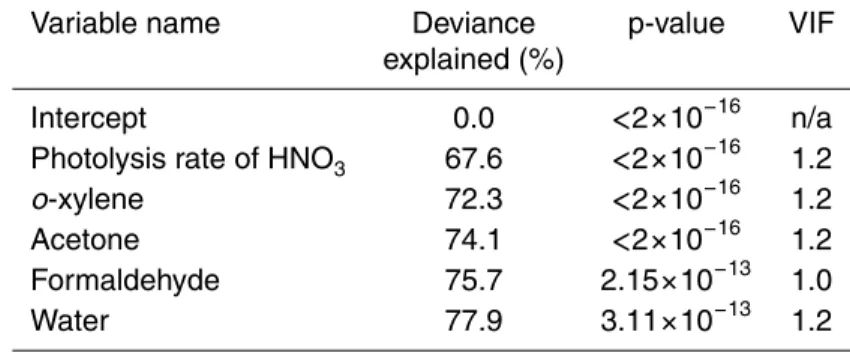
Table 2 shows the deviance explained by each variable: the photolysis rate for nitric acid was the most important predictor variable. The p-value associated with each of the smoothed terms provides a measure of the significance of the relationship for each predictor variable. All of the parameters were significant in explaining variation in measured OH concentrations at the 0.1% significance level. Collinearity was not a 15

concern as the variance inflation factors were less than the prescribed limit of five for all variables. The value for the intercept was 1.32×106molecule cm−3, the mean value of the measured OH radical concentrations. When the constant intercept is removed from the model, the deviance explained is reduced to just 24.7%. As well as assessing the significance of the predictor variables through p-values, the relationship between 20

the smoothed function of each predictor variable and the OH concentration was also explored (Fig. 3).

The photolysis reaction selected for GAMME was

HNO₃₊hν_→OH₊NO₂ (R1)

Figure 3a shows that the value of the smooth increases almost linearly with increas-25

(10)

ACPD

8, 14607–14642, 2008

additive models

Title Page

Tables Figures

◭ ◮

Back Close

Full Screen / Esc

be treated with caution owing to the limited amount of data as shown by the rug plot. The negative values of the smooth occur in periods when photolysis rates and OH radical concentrations were both low, for example at night-time. Whilst the photolysis rate for reaction (R1) produces the highest level of deviance explained, all of the pho-tolysis variables have similar explanatory power and all would have been suitable for 5

including in the model. In terms of interpretation, therefore, emphasis is placed on the role of photolytic reactions in general which act as sources of OH radicals rather than the role of the specific nitric acid photolysis reaction. The linear relationship (Fig. 3a) reflects the formation of OH radicals through a number of reactions when photolysis is important. For instance, OH can also be formed through photolysis of O3and HONO:

10

O3+hν→O1D+O2at wavelengths <320nm (R2)

O1D+H2O→2OH (R3)

HONO+M+hν→OH+NO+M (R4)

and also indirectly as peroxy radicals are formed e.g. through the photolysis of car-bonyl species (formaldehyde R5 and acetaldehyde R6):

15

HCHO+hν(+O2)→CO+2HO2 (R5)

CH3CHO+hν(+2O2)→HO2+CH3O2+CO (R6)

CH3O2+NO→CH3O+NO2 (R7)

CH3O+O2→HCHO+HO2 (R8)

HO2+NO→OH+NO2 (R9)

20

(11)

ACPD

8, 14607–14642, 2008

additive models

Title Page

Tables Figures

◭ ◮

Back Close

Full Screen / Esc

o-xylene is an aromatic hydrocarbon, a primary pollutant principally emitted by road vehicles through incomplete fuel combustion and fuel evaporation. During the day the degradation ofo-xylene is typically initiated through reaction with OH radicals, witho -xylene having a lifetime with respect to OH of approximately 20 h based on the average diurnal OH radical concentration during TORCH.

5

As theo-xylene concentration increases (Fig. 3b), the OH concentration decreases, a relationship that would be expected with any primary emitted species (i.e.o-xylene has no secondary sources in the atmosphere). For o-xylene concentrations greater than about 8×108molecule cm−3, the relationship with OH is broadly flat. The start of the plateau region may indicate that the atmosphere switches from VOC dependence 10

to NO_x dependence, and so any further increases in o-xylene concentration beyond this point have little impact on OH concentrations. The change in shape beyond a con-centration of 3×109molecule cm−3should not be over-interpreted due to the paucity of data and wide confidence intervals.

There is also a fairly simple relationship with acetone (Fig. 3c). With increasing 15

concentrations of acetone, the smooth initially increases in value indicating an asso-ciated increase in OH radical concentration. Beyond about 2.5×1010molecule cm−3 the smooth is broadly flat indicating no further impact on OH radical concentrations. Changes in shape at high concentrations of acetone should be treated with caution due to the limited volume of data on which the smooth is based.

20

Acetone is formed in the atmosphere through primary emissions from various bio-genic and anthropobio-genic sources and also through the oxidation of VOCs (Goldstein and Schade, 2000). For instance, the oxidation of propane and branched chain alka-nes, branched chain alkenes and oxygenated species all contribute to acetone pro-duction in the atmosphere. Biogenic sources includeα andβ-pinene and 2-methyl-3-25

buten-2-ol, which have acetone yields of 8–15% and 50% respectively (Goldstein and Schade, 2000).

(12)

ACPD

8, 14607–14642, 2008

additive models

Title Page

Tables Figures

◭ ◮

Back Close

Full Screen / Esc

reaction:

OH+CH3COCH3+O2→CH3COCH2O2+H2O (R10)

The peroxy radical formed in R10 can undergo reaction with NO, other RO2or HO2

to form a variety of products. However, under the TORCH conditions, reaction with NO is most likely (Emmerson et al., 2007):

5

CH₃COCH₂O₂+NO→CH3COCH2O+NO2 (R11)

The CH3COCH2O radical decomposes very quickly to the peroxyacetyl (CH3CO3)

radical and formaldehyde:

CH3COCH2O→CH3CO3+HCHO (R12)

The HCHO feeds back to OH through R5 and R9. The CH₃CO₃radical reacts with 10

NO to form CH3O2(R13), which itself feeds back to OH through R7-R9:

CH3CO3+NO+O2→CH3O2+NO2+CO2 (R13)

Alternatively, the acetone can undergo photolysis to form CH3O2and CH3CO3

radi-cals:

CH₃COCH₃₊hν_→CH₃CO₃₊CH₃O₂ (R14)

15

These radicals will then regenerate OH through R13, and R7-R9. The photolysis of acetone is therefore a radical and ultimately an OH source. The impact on OH of its reaction with acetone will depend on the acetone and NO concentrations. For the data used to construct the GAM, the destruction rate of acetone through photolysis is 5.0×103molecule cm−3s−1 on average, compared with an OH destruction rate of 20

(13)

ACPD

8, 14607–14642, 2008

additive models

Title Page

Tables Figures

◭ ◮

Back Close

Full Screen / Esc

However, both of these destruction rates become insignificant when considering the production rate of acetone through VOC oxidation. Although it is not possible to know for sure the production rate of acetone in the atmosphere during TORCH, particularly given that the biogenic species were not measured, a lower limit can be estimated from the relevant measured hydrocarbons that go on to form acetone when they de-5

grade. These are i-butene, i-pentane, propane,o-xylene, 2-methyl-2-butene, i-butane, 2-methylpentane, propanol and 2,2-dimethylbutane. The combined production rate from these 9 species is 1.2×105molecule cm−3s−1, almost a factor of 10 more im-portant than the combined destruction rates through reaction with OH and photolysis, despite this rate being a lower limit for reasons stated above. There is net produc-10

tion of acetone during TORCH, therefore, and the behaviour observed in Fig. 3c can be explained through OH and acetone being formed through the same degradation processes in the atmosphere.

Figure 3d shows the profile of HCHO with OH. The tails of the smooth should be interpreted with caution due to the paucity of data and wide confidence intervals. 15

Formaldehyde is both a primary pollutant (directly emitted from combustion processes for instance) and a secondary pollutant (from the degradation of hydrocarbons). There are two competing reactions to consider for HCHO destruction, photolysis (R5) and reaction with OH (R15):

HCHO₊OH(₊O₂)→CO+HO2+H2O (R15)

20

Under the conditions considered, the average rate of R5 was 2.9×105molecule cm−3s−1, whilst that of R15 was 4.5×105molecule cm−3s−1. Therefore, reaction with OH is ∼1.5 times more important than photolysis in terms of HCHO destruction. As the HCHO concentration increases, the rate of R15 will increase, which may be expected to suppress the OH concentration. However, R5 and 25

R15 produce HO2 radicals, which will subsequently reform OH through R9. These

(14)

ACPD

8, 14607–14642, 2008

additive models

Title Page

Tables Figures

◭ ◮

Back Close

Full Screen / Esc

where there are more data points, it appears that as the HCHO concentration in-creases that of OH dein-creases. The smooth, therefore, indicates that the destruction of formaldehyde through reaction with OH radicals is more important than formaldehyde regeneration through hydrocarbon oxidation.

Water plays a complex role in atmospheric chemistry affecting the rates of a wide 5

range of reactions and is present in relatively large concentrations. The smooth re-flects this complexity (Fig. 3e) with increases in water concentration associated with both increasing and decreasing OH radical concentrations. Owing to the forma-tion of OH through R2 and R3, it may be expected that as the water concentra-tion increases, so does that of OH. Indeed, at lower concentraconcentra-tions of H₂O, the OH 10

does increase with H₂O. However, as the H₂O concentration increases past about 2.7×1017molecule cm−3, the OH concentration begins to decrease. Such variations probably indicate that there are physical processes occurring that are impacting the OH, perhaps to do with temperature effects, or aerosol formation, that are not immedi-ately obvious. These variations are also much less significant in explaining variations in 15

OH radical concentration than contributions from other smooth functions. Variations in the smooth function for photolysis rate, for example, are almost an order of magnitude greater than variations in the smooth for water.

3.2 TORCH Modelled OH (GAM_MO)

The GAM produced for the TORCH modelled OH data comprises a constant intercept 20

and five smooths as shown in Table 3.

The value of the intercept is 1.63×106molecule cm−3, the mean value of modelled OH. Removing the intercept from the GAM reduces the deviance explained from 83.1% to 27.6%. The observed relationship between the smoothed function of each predictor variable and the OH concentration is shown in Fig. 4. Collinearity was not a concern as 25

(15)

ACPD

8, 14607–14642, 2008

additive models

Title Page

Tables Figures

◭ ◮

Back Close

Full Screen / Esc

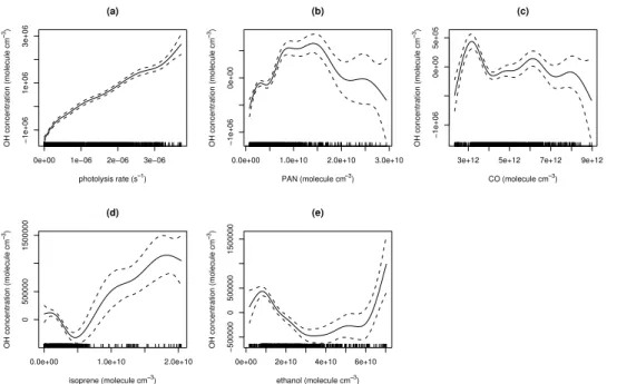
The photolysis rate included in GAM_MOrepresents the following reaction:

CH₃CHO+hν(+O₂)→HO2+CH3O2 (R16)

As for measured OH, the smooth increases with photolysis rate in a broadly linear manner (Fig. 4a). As with GAMME, the specific photolysis reaction is not particularly

important as all photolysis variables had a similar level of explanatory power and similar 5

smooths. The important point is that as photolysis rates increase, so do OH concen-trations consistent with photolytic reactions acting as a source of OH radicals.

Peroxyacetyl nitrate (PAN) is a secondary pollutant produced from the reaction of the CH₃CO₃radical with NO₂(Baird and Cann, 2005):

CH₃CO₃+NO₂⇋CH₃CO₃NO₂ (R17)

10

CH₃CO₃ is produced through the degradation of many hydrocarbons in the atmo-sphere. The formation of PAN generally peaks in the late afternoon when concentra-tions of hydrocarbons and OH radicals are relatively high and concentraconcentra-tions of nitric oxide are relatively low (as NO also reacts with the CH₃CO₃ radical, R13). Figure 4b shows that PAN behaves as a typical secondary pollutant, increasing as the concen-15

tration of OH increases, showing that both of these species are formed through photo-chemical processes. The smooth flattens as the PAN concentrations increase beyond 1.0×1010molecule cm−3, although there are fewer data here and the smooth should be interpreted with caution.

Carbon monoxide plays a significant role in OH radical chemistry. It can react with 20

OH radicals to produce HO2 radicals (Fig. 1), but is also produced as a by-product of

reactions involving the OH radical. For example, the degradation of hydrocarbons by OH radicals can lead to the formation of formaldehyde which produces carbon monox-ide on reaction with OH radicals (R15) or when broken down through photolysis (R5). Carbon monoxide is also a primary pollutant emitted from vehicle engines on incom-25

(16)

ACPD

8, 14607–14642, 2008

additive models

Title Page

Tables Figures

◭ ◮

Back Close

Full Screen / Esc

during each day due to the build-up of primary emissions and secondary production during the TORCH campaign. Low CO concentrations would be expected to be as-sociated with low OH radical concentrations as both occur in the early morning. The shape of the smooth in Fig. 4c shows that there is a complex relationship between CO and OH for the reasons stated above.

5

Isoprene is a hydrocarbon whose rate of emission increases strongly with increases in temperature. It behaves as a primary pollutant with emissions from both plants and road tra_ffic. Its fate in the environment is degradation through reaction with OH and NO3radicals, as well as through reaction with ozone. This behaviour is reflected

in the smooth in Fig. 4d which shows reducing OH values with increasing isoprene 10

concentrations where the majority of the data exist. The higher values for the smooth result mainly from late morning and early afternoon observations on a single day when OH radical concentrations were particularly high, probably due to high photolysis rates. Ethanol is a primary pollutant; a volatile organic hydrocarbon emitted through solvent usage and other industrial processes. Its fate in the atmosphere is to react with OH 15

radicals producing a range of secondary pollutant products such as acetaldehyde. The smooth (Fig. 4e) fits the shape of a primary pollutant with decreasing values associated with increasing concentration of ethanol as the ethanol acts as a sink for OH radicals.

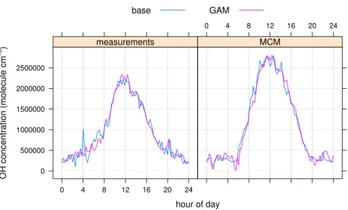
3.3 Prediction of OH radical concentrations

GAMME and GAMMO were validated by using them to predict OH radical

concentra-20

tions. A bootstrapping approach was used which involved 1000 repeated samples from the data. Each sample, comprising 75% of the data, was used to calibrate the GAM model. The calibrated GAM was then used to predict OH concentrations for the remaining 25% of the data. Figure 5 shows that the predicted values from GAM_ME and GAMMO closely approximated the diurnal distribution of measured OH and modelled

25

OH concentrations.

(17)

ACPD

8, 14607–14642, 2008

additive models

Title Page

Tables Figures

◭ ◮

Back Close

Full Screen / Esc

mean diurnal OH concentration whereas the MCM model over-estimated by 16.3%. The root mean squared error (RMSE) of GAMME, as a proportion of the mean diurnal

concentration, was appreciably lower than the RMSE of the MCM model.

The accuracy of predictions produced by GAMs may be compromised by the pres-ence of autocorrelation. Examination of correlograms for measured OH on each day 5

showed them to be autocorrelated and was confirmed by the Durbin-Watson test. The autocorrelation coefficient at lag 1 was 0.45 for the residuals of GAM_ME compared to 0.85 for the measured OH data. For the residuals of GAMMO and modelled OH data,

the autocorrelation coefficients at lag 1 were 0.54 and 0.93, respectively. Fitting auto-regression models (AR) to the measured OH data for each day and minimising the 10

Akaike Information Criterion provided an estimate of the order of each AR process. The order was found to be 1 on 15 of the 22 days with values ranging from 0 to 8 on other days. The residuals for GAM_ME also exhibited autocorrelation with the estimated order of the AR processes varying between 0 and 8 for individual days. The GAM_ME model only eliminated autocorrelation in 6 of the 21 days on which it was originally 15

present in the measured OH data.

4 Discussion

The shape of the smooths provides a general description of the role played by an individual variable. All the photolysis variables exhibited an approximate positive linear relationship with OH radical concentrations. The primary pollutants broadly displayed 20

an inverse relationship between the concentration of the pollutant and the concentration of OH radicals. At low concentrations, the secondary pollutants generally showed a positive correlation between pollutant concentration and OH radical concentration. At medium to high concentrations the shape of the smooth generally became flat around the zero level. Whilst the shapes of the functions can provide an indication of the 25

(18)

ACPD

8, 14607–14642, 2008

additive models

Title Page

Tables Figures

◭ ◮

Back Close

Full Screen / Esc

Table 5 shows that both models have a photolysis variable which is the most impor-tant in terms of deviance explained ( 67–69%). It is so imporimpor-tant that a GAM model comprising only the photolysis variable produced predictions of measured OH concen-tration almost as good as the five variable GAMME model (see Table 4). The deviance

explained by all photolysis variables was very high compared to other variables. There 5

was also little difference between the variable selected for a GAM and the remaining photolysis variables. Photolysis is clearly important as it is a strong source for OH rad-icals both directly and indirectly. As well as having a photolysis variable, both models included a mixture of primary and secondary pollutants. Interestingly, the two GAMs contained no common species.

10

The location of the TORCH experiment was a semi-rural environment with significant atmospheric emissions from plants and trees. Such emissions would have been ac-celerated by the high temperatures experienced that summer, which may explain the presence of acetone and isoprene in these models, both of which can be emitted in part from biogenic sources. As with all of the variables, they do not solely represent 15

the contribution of that named chemical but represent the role played by a range of species that exhibit broadly similar behaviour.

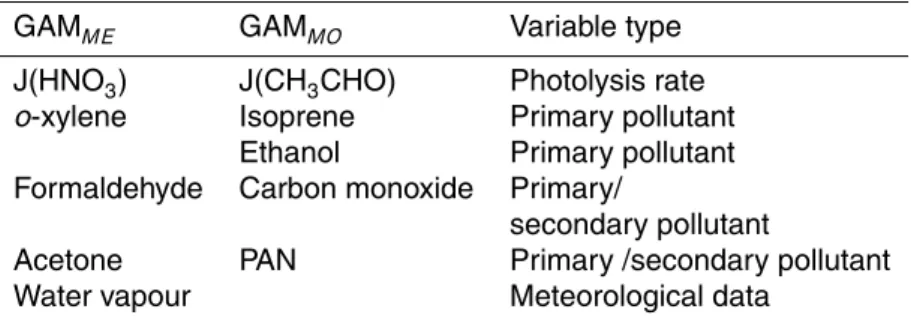
So what can the results tell us? For the measurements, the results suggest that

o-xylene, acetone, formaldehyde and water vapour are important, whilst for the model, isoprene, CO, PAN and ethanol affect the OH. Isoprene concentrations were remark-20

ably high during the TORCH campaign, which explains the impact on the model re-sults. However, its lack of impact on the measurements is surprising. This difference may reflect the fact that isoprene was just one of many biogenic species present dur-ing TORCH (unfortunately, no others were measured). It may only have represented a small proportion of the biogenic carbon present and as such, may only have had a 25

(19)

ACPD

8, 14607–14642, 2008

additive models

Title Page

Tables Figures

◭ ◮

Back Close

Full Screen / Esc

is not representative of some other biogenic hydrocarbons.

Another interesting di_fference is that the measurements show a dependence ono -xylene concentrations, whilst those of the model do not. There are known to be de-ficiencies with how the aromatic degradation schemes are represented in the MCM (Jenkin et al., 2003). The fact that the measured OH concentrations show a depen-5

dence on an aromatic species whilst the modelled OH values do not, may suggest that this area still needs work.

Although it is possible to read too much into the di_fferences at this stage, it is interest-ing that differences in the dependencies of modelled and measured OH concentrations exist, other than those previously noted for NOX. Trying to understand the reason for

10

such di_fferences may help us to understand what causes modelled and measured OH concentrations to differ so significantly on occasion.

The fit of the GAM models to the data was good and the predictions of OH concen-trations were an improvement over the MCM model. The model prediction approach using bootstrapping ensured that these predictions were based on data not used in 15

the model construction reinforcing the credibility of the validated models. There re-main limitations, however, with the results from the GAM models. Two sources of error were prominent in the model residuals. Firstly, extremely high OH concentrations were under-estimated by both GAMME and GAMMO. Figure 6 shows that all observations

greater than 4×106molecule cm−3were under-estimated by GAMME. The discrepancy

20

is substantial with the mean value of these observations being under-estimated by 27%. Observations at very high and also very low concentrations were not as accu-rately estimated as observations close to the mean level. The GAM models, therefore, appear to provide a less robust description of the atmospheric chemistry at these ex-tremes.

25

(20)

ACPD

8, 14607–14642, 2008

additive models

Title Page

Tables Figures

◭ ◮

Back Close

Full Screen / Esc

hour record of measurements over a greater number of days may resolve this issue without recourse to increasing the number of constant parameters.

Predictions produced by the GAM models, as well as being biased by errors asso-ciated with extremely high OH concentrations and by observations that immediately follow a gap in the measurement time series, are also prejudiced by autocorrelation in 5

the data. This is not surprising. TORCH time series data were averaged or interpo-lated to give measurements at intervals of 15 min. OH radical concentrations and the concentrations of many atmospheric gases also follow a systematic diurnal pattern.

Autocorrelation could have been addressed by incorporating an explicitly defined autocorrelation process into the GAM models. The improvement in predictive capability 10

was weighed against the practical di_fficulty of modelling the numerous autocorrelation processes present. Furthermore, even without explicitly defining the autocorrelation processes the GAM models explained some of the autocorrelation. For example, the autocorrelation at lag 1 was reduced by almost 50% by both GAM_ME and GAM_MO. The predictions achieved in Fig. 5 were judged adequate for this research so no adjustment 15

was made. Further, the presence of autocorrelation had no effect on use of GAMME

and GAM_MOfor interpreting relationships and trends in the data.

5 Conclusions

The GAM methodology successfully produced models of measured and modelled OH radical concentrations for the TORCH experiment. GAM_ME, the model for measured 20

OH, explained 77.9% of the variation in the data and GAMMO, the model for modelled

OH, explained 83.1%. When used to predict OH concentrations the GAMME model

produced better results than the MCM model. GAM_ME accurately predicted the diur-nal profile of OH concentrations and the predicted mean diurdiur-nal concentration from GAMME under-estimated the measured mean by only 0.2% compared to 16.3%

over-25

(21)

ACPD

8, 14607–14642, 2008

additive models

Title Page

Tables Figures

◭ ◮

Back Close

Full Screen / Esc

The main weaknesses in the fit of the GAMs were, firstly, a consistent under prediction of very high OH observations, and secondly, relatively large residual errors for obser-vations immediately following a gap in the measurement time-series. The second point may be related to autocorrelation in the time-series data which was not allowed for in the GAM models. Whilst the predictions achieved using GAMME and GAMMO were

5

adequate for this research, autocorrelation may be sufficiently influential in other data to require explicit modelling within GAM models before they can be used for prediction purposes. Weaknesses in the fit of GAMME and GAMMOand the presence of

autocor-relation in the data did not affect use of these models for interpretation of trends and relationships in the atmospheric chemistry. Both models identified the key role played 10

by photolysis reactions in the generation of OH radicals with photolysis variables ex-plaining between 67% and 69% of the variation in OH concentrations. Both models also included a combination of primary and secondary pollutants. Due to the statisti-cal nature of the GAM models, chemistatisti-cal parameters selected for GAM_ME and GAM_MO were not interpreted as possessing unique properties but properties representative of 15

a range of species. Care was also required not to over-interpret the shapes of smooth functions for parts of the curves where there were limited data. In general, primary pollutants were found to act as sinks for OH radicals with high concentrations of the pollutant associated with low concentrations of the OH radical. Secondary pollutants were generally found to have a positive correlation with OH radicals at low concen-20

trations. At medium to high concentrations, OH radicals were broadly insensitive to changes in concentration of the secondary pollutants.

Besides the photolysis variables, GAM_ME suggested that o-xylene, acetone, formaldehyde and water vapour were influential for OH concentrations and GAMMO

suggested that isoprene, CO, PAN and ethanol were influential. The differences 25

in these dependencies of modelled and measured OH concentrations supplements knowledge of differences for NOX already noted by Emmerson et al. (2007). Of

partic-ular interest were: the inclusion ofo-xylene in GAMME and not in GAMMOwhen there

(22)

ACPD

8, 14607–14642, 2008

additive models

Title Page

Tables Figures

◭ ◮

Back Close

Full Screen / Esc

et al., 2003); and, the inclusion of acetone in GAM_ME apparently as an indicator of biogenic processing whilst it was ‘replaced’ by isoprene in GAMMO. The close fit to the

data achieved by the GAM models and successful prediction of the diurnal profile of OH concentration supports the use of GAM models as a supplement to MCM modelling. More comprehensive data with measurements over much longer periods of time would 5

enhance the ability of GAMs to provide insight into the underlying atmospheric chem-istry and help address the problems encountered with observations that immediately follow gaps in the data.

GAM models have the potential to be applied more widely in modelling atmospheric chemistry. They are particularly suited to identifying trends in historic data, filling-in 10

gaps in measured data and supporting interpretation of the chemistry. They can be used to forecast future concentrations once the models have been calibrated for a specific location and once secular trends and autoregression have been addressed in the modelling.

Acknowledgements. We would like to thank all of the scientists involved with the TORCH

cam-15

paign. In particular we would like to thank the research group of Professor Dwayne Heard at the University of Leeds for providing the OH data. We would also like to thank the R software developers. The TORCH project was funded via NERC grant number NER/T/S/2002/00498. Lawrence Jackson was funded via a scholarship from the Environment Department of the Uni-versity of York.

20

References

Baird, C. and Cann, M.: Environmental Chemistry, 3rd edition, Freeman, 154, 2005. 14621 Bower, J., Lampert, J., Broughton, G., Stedman, J., Pye, S., Targa, J., Kent, A., and Grice, S.:

Air pollution in the UK, 13, 2005, 2006 . 14609

Carslaw, D. C. and Carslaw, N.: Detecting and characterising small changes in urban nitrogen

25

dioxide concentrations, Atmos. Environ., 41, 4723–4733, 2007. 14611

(23)

c-ACPD

8, 14607–14642, 2008

additive models

Title Page

Tables Figures

◭ ◮

Back Close

Full Screen / Esc

Interactive Discussion related emissions using a generalised additive modelling approach, Atmos. Environ., 41,

5289–5299, 2007. 14611

Chatfield, C.: The Analysis of Time Series: An Introduction, 4th edition, Chapman & Hall/CRC, 62, 1992. 14614

Creasey, D. J., Evans, G. E., Heard, D. E., and Lee, J. D.: Measurements of OH and HO₂

5

concentrations in the Southern Ocean marine boundary layer, J. Geophys. Res., 108(D15), 4475, doi:10.1029/2002JD003206, 2003. 14610

Emmerson, K. M., Carslaw, N., Carpenter, L. J., Heard, D. E., Lee, J. D., and Pilling, M. J.: Urban Atmospheric Chemistry During the PUMA Campaign 1: Comparison of Modelled OH and HO₂Concentrations with Measurements, J. Atmos. Chem., 52, 143–164, 2005. 14609,

10

14610

Emmerson, K. M., Carslaw, N., Carslaw, D. C., Lee, J. D., McFiggans, G., Bloss, W. J., Grave-stock, T., Heard, D. E., Hopkins, J., Ingham, T., Pilling, M. J., Smith, S. C., Jacob, M., and Monks, P. S.: Free radical modelling studies during the UK TORCH Campaign in Summer 2003, Atmos. Chem. Phys., 7, 167–181, 2007,

15

http://www.atmos-chem-phys.net/7/167/2007/. 14609, 14610, 14612, 14618, 14627

European Parliament and Council: Decision No 1600/2002/EC of the European Parliament and of the Council of 22 July 2002 laying down the Sixth Community Environment Action Programme, 2002. 14608

Freund, R. J. and Wilson, W. J.: Regression Analysis: Statistical Modeling of a Response

20

Variable, Academic Press, 193, 1998. 14614

Goldstein, A. H. and Schade, G. W.: Quantifying biogenic and anthropogenic contributions to acetone mixing ratios in a rural environment, Atmos. Environ., 34, 4997–5006, 2000. 14617 Hastie, T. J. and Tibshirani, R.: Generalized additive models, Chapman and Hall, London,

1990. 14611

25

Heard, D. E. and Pilling, M. J.: Measurement of OH and HO₂in the troposphere, Chem. Rev, 103, 5163–5198, 2003. 14609, 14610

Jenkin, M. E., Saunders, S. M., Wagner, V., and Pilling, M. J.: Protocol for the development of the Master Chemical Mechanism, MCM v3 (Part B): tropospheric degradation of aromatic volatile organic compounds, Atmos. Chem. Phys., 3, 181–193, 2003,

30

http://www.atmos-chem-phys.net/3/181/2003/. 14609, 14625, 14627

(24)

ACPD

8, 14607–14642, 2008

additive models

Title Page

Tables Figures

◭ ◮

Back Close

Full Screen / Esc

Interactive Discussion A., Bachmann, K., Schlomski, S., Moortgat, G., and Großmann, D.: Hydrocarbon

mea-surements at Pabstthum during the BERLIOZ campaign and modeling of free radicals, J. Geophys. Res., 108, 8251, 2003. 14611

Lee, J. D., Lewis, A. C., Monks, P. S., Jacob, M., Hamilton, J. F., Hopkins, J. R., Watson, N. M., Saxton, J. E., Ennis, C., Carpenter, L. J., Carslaw, N., Fleming, Z., Bandy, B. J.,

5

Oram, E., D., Penkett, S. A., Slemr, J., Norton, E., Rickard, A. R., Whalley, L. K., Heard, E., D., Bloss, W. J., Gravestock, T., Smith, S. C., Stanton, J., Pilling, M. J., and Jenkin, M. E.: Ozone photochemistry and elevated isoprene during the UK heatwave of August 2003, Atmos. Environ., 40, 7598–7613, 2006. 14609

McCullagh, P. and Nelder, J. A.: Generalized Linear Models, Chapman & Hall/CRC, 1989.

10

14611

Montgomery, D. C. and Peck, E. A.: Introduction to Linear Regression, Wiley, New York, 300, 1992. 14614

R Development Core Team: R: A Language and Environment for Statistical Computing, R Foun-dation for Statistical Computing, Vienna, Austria, http://www.R-project.org, ISBN

3-900051-15

07-0, 2007. 14613

Reiss, R.: Temporal trends and weekend-weekday differences for benzene and 1,3-butadiene in Houston, Texas, Atmos. Environ., 40, 4711–4724, 2006. 14611

Ren, X., Harder, H., Martinez, M., Lesher, R. L., Oliger, A., Simpas, J. B., Brune, W. H., Schwab, J. J., Demerjian, K. L., He, Y., Zhoud, X., , and Gao, H.: OH and HO₂Chemistry in the urban

20

atmosphere of New York City, Atmos. Environ., 37, 3639–3651, 2003. 14611

Saunders, S. M., Jenkin, M. E., Derwent, R. G., and Pilling, M. J.: Protocol for the development of the Master Chemical Mechanism, MCM v3 (Part A): tropospheric degradation of non-aromatic volatile organic compounds, Atmos. Chem. Phys., 3, 161–180, 2003,

http://www.atmos-chem-phys.net/3/161/2003/. 14609

25

Smith, S. C., Lee, J. D., Bloss, W. J., Johnson, G. P., Ingham, T., and Heard, D. E.: Concentra-tions of OH and HO₂radicals during NAMBLEX: measurements and steady state analysis, Atmos. Chem. Phys., 6, 1435–1453, 2006,

http://www.atmos-chem-phys.net/6/1435/2006/. 14610

Warneck, P.: Photodissociation of acetone in the troposphere: an algorithm for the quantum

30

(25)

ACPD

8, 14607–14642, 2008

additive models

Title Page

Tables Figures

◭ ◮

Back Close

Full Screen / Esc

Interactive Discussion Westmoreland, E., Carslaw, N., Carslaw, D., Gillah, A., and Bates, E.: Analysis of air quality

within a street canyon using statistical and dispersion modelling techniques, Atmos. Environ., 41, 9195–9205, 2007. 14618

Wood, S. N.: Generalized Additive Models: An Introduction with R, Chapman and Hall/CRC, 2006. 14611

(26)

ACPD

8, 14607–14642, 2008

additive models

Title Page

Tables Figures

◭ ◮

Back Close

Full Screen / Esc

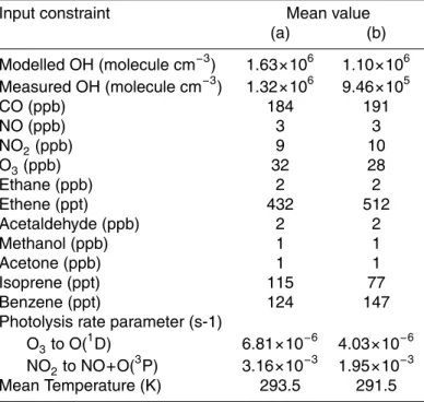
Table 1. Key input constraints for TORCH. (a)Mean value of all 933 data points. (b) Mean

diurnal value calculated using the mean values of observations recorded at the same time of day.

Input constraint Mean value

(a) (b)

Modelled OH (molecule cm−3₎ _1.63

×106 1.10×106 Measured OH (molecule cm−3₎ _1.32

×106 9.46×105

CO (ppb) 184 191

NO (ppb) 3 3

NO₂(ppb) 9 10

O₃(ppb) 32 28

Ethane (ppb) 2 2

Ethene (ppt) 432 512

Acetaldehyde (ppb) 2 2

Methanol (ppb) 1 1

Acetone (ppb) 1 1

Isoprene (ppt) 115 77

Benzene (ppt) 124 147

Photolysis rate parameter (s-1)

O₃to O(1D) 6.81×10−6 4.03×10−6 NO₂to NO+O(3P) 3.16×10−3 1.95×10−3

(27)

ACPD

8, 14607–14642, 2008

additive models

Title Page

Tables Figures

◭ ◮

Back Close

Full Screen / Esc

Table 2.TORCH measured OH (GAM_ME) results comprising the variables selected, deviance

explained, p-values for each variable and variance inflation factors. Deviance explained is shown as the cumulative total for each variable and the preceding variables.

Variable name Deviance p-value VIF

explained (%)

Intercept 0.0 <2×10−16 n/a

Photolysis rate of HNO₃ 67.6 <2×10−16 1.2 o-xylene 72.3 <2×10−16 1.2

Acetone 74.1 <2×10−16 1.2

Formaldehyde 75.7 2.15×10−13 1.0

(28)

ACPD

8, 14607–14642, 2008

additive models

Title Page

Tables Figures

◭ ◮

Back Close

Full Screen / Esc

Table 3. TORCH modelled OH (GAM_MO) results comprising the variables selected, deviance

explained, p-values for each variable and variance inflation factors. Deviance explained is shown as the cumulative total for each variable and the preceding variables.

Variable name Deviance p-value VIF

explained (%)

Intercept n/a <2×10−16 n/a

Photolysis rate of HNO₃ 68.3 <2×10−16 1.2

PAN 70.8 <2×10−16 1.4

Carbon monoxide 76.5 <2×10−16 2.8

Isoprene 80.6 <2×10−16 1.2

(29)

ACPD

8, 14607–14642, 2008

additive models

Title Page

Tables Figures

◭ ◮

Back Close

Full Screen / Esc

Table 4.Mean diurnal values and root mean squared error results for GAM and MCM models.

GAM_ME (photolysis) shows the results for GAM_ME with only the photolysis variable and the constant term present.

TORCH Mean diurnal value RMS error

(molecule cm−3₎ _{(molecule cm}−3₎

Measured concentration 9.46×105 n/a

MCM model 1.10×106 8.87×105

GAM_ME 9.44×105 1.39×105

GAM_MO 1.09×106 1.32×105

(30)

ACPD

8, 14607–14642, 2008

additive models

Title Page

Tables Figures

◭ ◮

Back Close

Full Screen / Esc

Table 5.GAM predictor variables classified by type.

GAM_ME GAM_MO Variable type

J(HNO₃) J(CH₃CHO) Photolysis rate o-xylene Isoprene Primary pollutant

Ethanol Primary pollutant Formaldehyde Carbon monoxide Primary/

secondary pollutant

Acetone PAN Primary /secondary pollutant

(31)

ACPD

8, 14607–14642, 2008

additive models

Title Page

Tables Figures

◭ ◮

Back Close

Full Screen / Esc

Interactive Discussion O1_D

O₃

OH

RO₂ ROOH

RCHO

HO

₂ H₂O₂

RO HC

hv

NO

NO HO₂

O₂ O₃

O₃ HO2

OH CO

H₂ H₂O

NO

HONO HNO₃

NO₂ NO

hv

RO₂

Fig. 1. Schematic of the key reactions of the OH radical in the atmosphere. The green lines

(32)

ACPD

8, 14607–14642, 2008

additive models

Title Page Abstract Introduction Conclusions References Tables Figures ◭ ◮ ◭ ◮ Back Close

Full Screen / Esc

photolysis rate (s

−−1

)

OH concentration (molecule cm

−− 3

)

0e+00 1e+06 2e+06 3e+06 4e+06 5e+06 6e+06

0.0e+00 5.0e−06 1.0e−05 1.5e−05 2.0e−05 2.5e−05

● ● ● ● ● ● ● ● ● ● ● ● ● ● ●● ● ● ● ● ● ● ● ● ● ● ● ● ● ● ● ● ● ● ● ● ● ● ● ● _● ● ● ●● ●● ● ● ● ● ● ● ● ● ● ● ● ● ● ● ● ● ● ● ● ● ● ● ● ● ●_● ● ● ● ● ● ● ● ● ● ● ● ● ● ● ● ● ● ● ● ● ● ● ● ● ● ● ● ● ● ● ● ● _● ● ● _● ● ● ● ● ● ● ● ● ● ● ● ● ● ● ● ● ● ● ● ● ● ● ●●_●● ●● ● ● ● ● ● ● ● ● ●●● ● ● ● ●● ● ● ● ● ● ● ● ● ● ● ● ● ● ● ● ● ● ● ● ● ● ●●●●●● ● ● ● ● ● ● ● ● ● ● ● ● ● ● ● ● ● ● ● ● ● ● ● ● ● ● ● ● ● ● ● ● ● ● ● ● ● ● ● ● ● ● ● ● ● ● ● ● ● ● ● ● ● ● ● ● ● ● ● ● ● ● ● ● ● ● ● ● ● ● ● ● ● ● ● ● ● ● ● ● ● ● ● ● ● ● ● ●● ● ●● ●● ●● ● ● ● ● ● ● ● ● ● ● ● ● ● ● ● ● ● ● ● ● ● ● ● ● ● ● ● ● ● ● ● ● ● ● ● ● ● ● _● ● ● ● ● ● ●_● ● ● ● ● ● ● ● ●●●● ● ● ● ● ● ● ● ● ● _● ● ● ● ● ● ● ● ● _● ● ● ● ●● ● ● ● ● ● ● ● ● ● ● ● ● ● ● ● ● ● ● ● ● ●● ● ● ● ● ● ●●● ● ● ● ● ● ● ● ● ● ● ● ● ● ●● ● ● ●_●● ●● ● ● ● ● ● ● ● ● ● ● ● ● ● ● ● ● ● ● ● ● ● ● ● ● ● ● ● ● ● ● ● ● ● ● ● ● ● ● ● ● ● ● ● ● ● ● ● ● ● ●● ● ● ● ● ● ● ● ● ● ● ● ● ● ● ● ● ● ● ● ● ● ●● ● ● ● ● ● ●● ● ● ● ● ● ● ● ● ● ● ● ● ● ● ● ● ● ● ● ● ● ● ●● ● ● ● ● ● ● ● ● ● ●● ● ● ● ●● ● ● ● ● ● ●● ● ● ● ● ● ● ● ● ● ● ● ●● ● ● ● ● ● ● ● ● ● ● ● ● ● ● ● ● ● ● ● ● ● ● ● ● ● ● ● ● ●_● ●● ● ● ● ● ● ● ● ● ● ● ● ● ● ● ● ● ● ● ● ● ● ● ● ● ● ● ● ● ● ● ●● ●● ● ● ● ● ● ●●● ● ● ● ● ● ● ● ● ● ● ● ● ● ● ● ● ●● ● ● ● ● ● ● ● ● ● ● ● ● ● ● ● ● ● ● ● ● ● ● ● ● ● ● ● ● ● ● ● ● ● ● ● ● ● ● ● ●● ● ● ● ● ● ● ● ● ● ● ● ● ● ● ● ● ● ● ● ● ● ● ● ● ● ● ● ● ● ● ● ● ● ● ● ●● ● ● ● ● ● ● ● ● ● ● ● ● ● ● ● ● ● ● ● ● ● ● ● ● ● ● ● ● ● ● ●●● ●●●●● ● ● ● ● ● ● ● ● ● ● ● ● ● ● ● ● ● ● ● ● ● ● ● ● ● ● ● ● ● ● ● ● ● ● ● ● ● ● ● ● ● ● ● ● ● ● ● ● ● ● ● ● ● ● ● ● ● ● ● ● ● ● ● ● ● ● ●● ● ● ● ●● ●● ●●●●● ● ● ● ● ● ● ● ● ● ● ● ● ● ● ● ● ● ● ● ● ●● ● ● ● ● ● ● ● ● ● ● ● ● ● ● ● ● ● ● ● ● ● ● ● ● ● ● ● ● ● ● ● ●● ●● ● ● ● ● ●● ● ● ● ● ●● ● ● ● ● ● ● ● ● ● ● ● ● ●● ● ●●● ● ● ● ● ● ● ● ●

Fig. 2.Specimen smooth for OH concentration (molecule cm−3_{), the response variable, plotted}

against the photolysis rate of O₃(to form O(1D)) (s−1_{), the predictor variable. The original data}

(33)

ACPD

8, 14607–14642, 2008

additive models

Title Page

Tables Figures

◭ ◮

Back Close

Full Screen / Esc

Interactive Discussion 0e+00 2e−07 4e−07

−1e+06

1e+06

3e+06

(a)

photolysis rate (s−−1)

OH concentration (molecule cm

−−

3)

0e+00 1e+09 2e+09 3e+09 4e+09

−5e+05

5e+05

(b)

o−xylene (molecule cm−−3)

−−

3)

2e+10 4e+10 6e+10 8e+10 1e+11

−1e+06

0e+00

1e+06

(c)

acetone (molecule cm−−3₎

−−

3)

1e+10 3e+10 5e+10 7e+10

−8e+05

−2e+05

4e+05

(d)

formaldehyde (molecule cm−−3₎

−−

3)

2.5e+17 3.5e+17 4.5e+17

−6e+05

−2e+05

2e+05

(e)

water (molecule cm−−3₎

−−

3)

Fig. 3. Smooth functions of the predictor variables for measured OH(a)photolysis rate,(b)

(34)

ACPD

8, 14607–14642, 2008

additive models

Title Page

Tables Figures

◭ ◮

Back Close

Full Screen / Esc

0e+00 1e−06 2e−06 3e−06

−1e+06

1e+06

3e+06

(a)

photolysis rate (s−−1)

−−

3)

0.0e+00 1.0e+10 2.0e+10 3.0e+10

−1e+06

0e+00

(b)

PAN (molecule cm−−3)

−−

3)

3e+12 5e+12 7e+12 9e+12

−1e+06

0e+00

5e+05

(c)

CO (molecule cm−−3)

−−

3)

0.0e+00 1.0e+10 2.0e+10

0

500000

1500000

(d)

isoprene (molecule cm−−3₎

−−

3)

0e+00 2e+10 4e+10 6e+10

−500000

0

500000

1500000

(e)

ethanol (molecule cm−−3₎

−−

3)

Fig. 4. Smooth functions of the predictor variables for modelled OH(a) photolysis rate, (b)

(35)

ACPD

8, 14607–14642, 2008

additive models

Title Page

Tables Figures

◭ ◮

Back Close

Full Screen / Esc

hour of day

−−

3 )

0 500000 1000000 1500000 2000000 2500000

0 4 8 12 16 20 24

measurements

0 4 8 12 16 20 24

MCM

base GAM

Fig. 5. Comparison of the measured (or modelled) OH concentration (shown as a blue line)