Comput. Appl. Math. vol.31 número1

Copyright © 2012 SBMAC

ISSN 0101-8205 / ISSN 1807-0302 (Online) www.scielo.br/cam

On a linearisation method for

Reiner-Rivlin swirling flow

ZODWA G. MAKUKULA, PRECIOUS SIBANDA* and SANDILE S. MOTSA

School of Mathematical Sciences, University of KwaZulu-Natal, Private Bag X01, Scottsville 3209, Pietermaritzburg, South Africa

E-mails: makukulaz@yahoo.com / sibandap@ukzn.ac.za / sandilemotsa@gmail.com

Abstract. The steady flow of a Reiner-Rivlin fluid with Joule heating and viscous dissipation is studied. We present a novel technique for accelerating the convergence of the spectral-homo-topy analysis method. Solutions of the nonlinear momentum and energy equations are obtained using the improved spectral homotopy analysis method. Solutions were also generated using the spectral-homotopy analysis method and benchmarked against results in the literature.

Mathematical subject classification: Primary: 76A05, 76N05; Secondary: 76M25. Key words: Reiner-Rivlin fluid, Chebyshev spectral method, spectral-homotopy analysis method, improved spectral-homotopy analysis method.

1 Introduction

The boundary layer induced by a rotating disk arises in many engineering appli-cations, for example, in computer storage devices, viscometry, turbo-machinery and in crystal growth processes (Attia [4]). Since the pioneering study by von Kármán [39], research on swirling flows has been carried out by, among others, Cochran [15] who proposed an improved solution to the von Kármán formula-tion based on a mixture of analytical and numerical techniques. Benton [12] studied the impulsive rotation from rest of a disk in an infinite viscous fluid. He improved Cochran’s solutions by first expanding the variables in a power series

and solving for the first two orders analytically, and then numerically computing the next two orders.

2 Equations

We consider an infinite rotating disk coinciding with the planez =0 with the space z > 0 occupied by a viscous, incompressible Reiner-Rivlin fluid. The fluid motion and heat transfer are governed by the equations (see [4, 5, 33]);

∂u ∂r +

u

r +

∂w

∂z =0, (1)

ρ

u∂u ∂r +w

∂u ∂z −

v2

r

+σB₀2u₌ ∂τ

r r

∂r + ∂τz

r

∂z + τr

r −τ

φ φ

r , (2)

ρ

u∂v ∂r +w

∂v ∂z +

uv r

+σB₀2v₌ ∂τ

r

φ

∂r + ∂τ_φz

∂z +

2τ_φr

r , (3)

ρ

u∂w ∂r +w

∂w ∂z = ∂τ r z

∂r + ∂τz

z

∂z + τr

z

r , (4)

ρcp

u∂T ∂r +w

∂T ∂z =κ ₁ r ∂ ∂r

r∂T ∂r

+∂

2_T

∂z2 +μ ( ∂u ∂z 2 + ∂v ∂z 2)

+σB₀2(u2₊v2),

(5)

with the following no-slip boundary conditions

u ₌0, v₌r, w₌0, T ₌Tw at z ₌0 (6)

u _→0, v_→0, p_→ p_∞, T _→T_∞ as z _{→ ∞}, (7)

where the disk is rotating with a constant angular velocity  about the line

r ₌ 0 and an external uniform magnetic field is applied perpendicular to the plane of the disk with a constant magnetic flux density B0. The velocity com-ponents in the directions of increasingr, φ,z areu, v, w respectively. ρ is the density of the fluid, σ is the electrical conductivity of the fluid, μ is the co-efficient of viscosity, κ is the thermal conductivity, cp is the specific heat at

constant pressure of the fluid. The temperature of the fluid T, equals Tw at the surface of the disk. At large distances from the disk, T tends to T_∞where

side of equation (5) represents the viscous dissipation while the last term rep-resents the Joule heating. The constitutive equation for the Reiner-Rivlin fluid is given by

τi_{j =}2μei_{j +}2μceike k

j −pδ

i

j, e

j

j =0, (8)

where p represents the pressure, τi_j is the stress tensor, ei_j is the rate of strain tensor andμc is the coefficient of cross viscosity. The Reiner-Rivlin model is

a simple model which can provide some insight into predicting the flow char-acteristics and heat transfer performance for viscoelastic fluid above a rotating disk [6]. The first term on the right hand side of (8) represents the viscous prop-erty of the fluid and the third term, the elastic propprop-erty of the fluid. We introduce the non-dimensional distanceη =z√/νmeasured along the axis of rotation and the von Kármán transformations [39];

u₌rF, v₌rG, w₌√νH,

p− p∞= −ρνP, 2=

T ₋T_∞

Tw₋T_∞,

(9)

where F,G,H,P and2are non-dimensional functions of η,ν ₌ μ/ρis the kinematic viscosity. With these transformations equations (1)-(5) take the form

H′₊2F ₌0, (10)

F′′₋F2₊G2₋F′H₋M F₋ K

2 F ′2

−3G′2₋2F F′′₌0, (11)

G′′₋G′H ₋2F G₋M G₊K F′G′₊F G′′₌0, (12)

H H′₊7

2K H

′_H′′_−P′_−H′′ _{=0, (13)}

1

Pr2

′′

−H2′₊Ec F′2₊G′2₊M Ec F2₊G2₌0, (14)

with

F(0)= F(_∞)=0, G(0)=1, G(_∞)=0, H(0)=0, (15)

P(_∞)₌0, 2(0)₌1, 2(_∞)₌0, (16)

whereK ₌μc/μis the parameter that describes the non-Newtonian

charac-teristic of the fluid, M ₌ σB2

the Prandtl number andEcis the Eckert number. The system (10)-(12) with the prescribed boundary conditions (15) are sufficient to solve for the three velocity components. Equation (13) can be used to find the pressure distribution at any point if required. Simplifying the equation system by substituting equation (10) into (11), (12) and (14) yields

H′′′_−H′′_H+ 1 2H

′_H′_−2G2

−M H′

+ K 2

₁ 2H

′′2_−3G′2_−H′_H′′′

=0,

(17)

G′′−H G′+H′G−M G+ K 2(H

′_G′′_−H′′_G′_{)=0, (18)}

1

Pr2

′′

−H2′₊Ec

1 4H

′′2 +G′2

+M Ec

1 4H

′2 +G2

=0, (19)

subject to the boundary conditions

H(0)₌ H′(0)₌ H′(_∞)₌0, G(0)=2(0)=1, G(∞)=2(∞)=0.

(20)

In the following section we solve the nonlinear coupled system (17)-(19) with boundary conditions (20) by the ISHAM.

3 Method of solution

The main thrust of the method of solution [21, 28], is the improvement of the initial approximation used in the higher order deformation equations of the spec-tral homotopy analysis method. A systematic approach is used to find optimal initial “guesses” which are then used in the SHAM algorithm to accelerate con-vergence. In the first instance we assume that solutions for H(η), G(η) and

2(η)in equations (17)-(19) can be found in the form

H(η)₌hi(η)+ i−1 X

m=0

hm(η), G(η)=gi(η)+ i−1 X

m=0

gm(η),

2(η)₌θi(η)+ i−1 X

m=0

θm(η), i =1,2,3, . . . ,

wherehi, gi andθi are unknown functions whose solutions are obtained using

the SHAM approach at theith iteration andhm,gm andθm (m ≥ 1) are known

from previous iterations. For m ₌ 0, suitable initial guesses satisfying the boundary conditions (20) are

h0(η)= −1+e−η+ηe−η, g0(η)=e−η, θ0(η)=e−η. (22) The initial guesses (22) are improved upon as follows. Substituting (21) into the governing equations (17)-(19) gives

a0,i−1hi′′′+a1,i−1h′′i +a2,i−1h′i+a3,i−1hi +a4,i−1gi′+a5,i−1gi −h′′ihi

+1 2h

′

ih′i −2g

2

i +K

1 4h

′′2

i −3g′

2

i −

1 2h

′

ih′′′i

=r1,i−1,

(23)

b0,i−1g′′i +b1,i−1gi′+b2,i−1gi +b3,i−1h′′i +b4,i−1hi′+b5,i−1hi −higi′

+h′_igi−

K

2 h ′

ig′′i +h′′ig′i

=r2,i−1,

(24)

c0,i−1θi′′+c1,i−1θi′+c2,i−1h′′i +c3,i−1h′i +c4,i−1hi +c5,i−1gi′

+c6,i−1gi −Pr hiθi′+Ec Pr

1 4h

′′2

i +g′

2

i

+M Ec Pr

1 4h

′2

i +g

2

i

=r3,i−1,

(25)

subject to the boundary conditions

hi(0)=gi(0)=θi(0)=0, h′i(0)=h′i(∞)=0,

gi(∞)=θi(∞)=0.

(26)

The coefficient parametersak,i−1,bk,i−1,ck,i−1(k =0, . . . ,6),r1,i−1,r2,i−1and

r3,i−1are defined as

a0,i−1=1−

K

2

i−1 X

m=0

h′_m, a1,i−1=

K

2

i−1 X

m=0

h′′_{m −}

i−1 X

m=0

hm, (27)

a2,i−1=

i−1 X

m=0

h′_m−M₋ K

2

i−1 X

m=0

h′′′_m a3,i−1= −

i−1 X

m=0

a4,i−1= −6K

i−1 X

m=0

g′m a5,i−1= −4

i−1 X

m=0

gm, (29)

b0,i−1=1−

K

2

i−1 X

m=0

h′_m, (30)

b1,i−1= −

i−1 X

m=0

hm−

K

2

i−1 X

m=0

h′′_m,b2,i−1=

i−1 X

m=0

h′_m−M, (31)

b3,i−1= −

K

2

i−1 X

m=0

gm′ , b4,i−1=

i−1 X

m=0

gm −

K

2

i−1 X

m=0

gm′′, (32)

b5,i−1= −

i−1 X

m=0

g′_m, (33)

c0,i−1=1, c1,i−1= −Pr

i−1 X

m=0

hm, c2,i−1= 1 2Ec Pr

i−1 X

m=0

h′′_m, (34)

c3,i−1= 1

2Pr EcM

i−1 X

m=0

h′_m, c4,i−1= −Pr

i−1 X

m=0

θ_m′, (35)

c5,i−1=2Ec Pr

i−1 X

m=0

g′m, c6,i−1=2Pr M Ec

i−1 X

m=0

gm, (36)

r1,i−1 = − "_i−1

X

m=0

h′′′_m−

i−1 X

m=0

h′′_m

i−1 X

m=0

hm+

1 2

i−1 X

m=0

h′_m

i−1 X

m=0

h′_m

−2

i−1 X

m=0

gm i−1 X

m=0

gm+K

1 4

i−1 X

m=0

h′′m i−1 X

m=0

h′′m

−3

i−1 X

m=0

g′_m

i−1 X

m=0

g′_m−1

2

i−1 X

m=0

h′_m

i−1 X

m=0

h′′′_m

!#

,

(37)

r2,i−1 = − "_i−1

X

m=0

g_m′′ ₋

i−1 X

m=0

hm i−1 X

m=0

g_m′ ₊

i−1 X

m=0

h′_m

i−1 X

m=0

gm

+K 2

i−1 X

m=0

h′_m

i−1 X

m=0

g′′_m−

i−1 X

m=0

h′′_m

i−1 X

m=0

g′_m

!#

,

r3,i−1 = − "_i−1

X

m=0

θm′′−Pr i−1 X

m=0

hm i−1 X

m=0

θm′

+ Pr Ec

 



i−1 X

m=0

h′′_m

!2 +

i−1 X

m=0

g′_m

!2 



+Pr M Ec

 



i−1 X

m=0

h′_m

!2 +

i−1 X

m=0

gm

!2 

 

.

(39)

Starting from the initial guesses (22), the subsequent solutionshi,gi andθi (i ≥

1) are obtained by recursively solving equations (23)-(25). To solve equations (23)-(25), we start by defining the following linear operators

Lh

Hi(η;q),Gi(η;q)

=a0,i−1

∂3Hi

∂η3 +a1,i−1

∂2Hi

∂η2 +a2,i−1

∂Hi

∂η

+a3,i−1Hi+a4,i−1

∂Gi

∂η +a5,i−1Gi,

(40)

Lg

Hi(η;q),Gi(η;q)

=b0,i−1

∂2Gi

∂η2 +b1,i−1

∂Gi

∂η +b2,i−1Gi

+b3,i−1

∂2Hi

∂η2 +b4,i−1

∂Hi

∂η +b5,i−1Hi,

(41)

Lθ

Hi(η;q),Gi(η;q), 2i(η;q)

=c0,i−1

∂22i

∂η2 +c1,i−1

∂2 ∂η

+c2,i−1

∂2Hi

∂η2 +c3,i−1

∂Hi

∂η +c4,i−1Hi+c5,i−1 ∂Gi

∂η +c6,i−1Gi,

(42)

whereq _{∈ [}0,1_]is the embedding parameter, and

Hi(η;q), Gi(η;q) and 2i(η;q)

are unknown functions. The zeroth order deformation equations are given by

(1−q)LhHi(η;q)−hi,0(η)=q~Nh[Hi(η;q),Gi(η;q)] −r1,i−1 , (1−q)LgGi(η;q)−gi,0(η)=q~Ng[Hi(η;q),Gi(η;q)] −r2,i−1 ,

where~_{is the non-zero convergence controlling auxiliary parameter and Nh,}

NgandNθ are nonlinear operators given by

Nh

Hi(η;q),Gi(η;q)

=Lh

Hi(η;q),Gi(η;q)

−Hi

∂2Hi

∂η2 + 1 2

∂Hi

∂η

2 −2G2

i −M

∂Hi

∂η +K ( 1 4

∂2Hi

∂η2 2

−3

∂Gi

∂η

2 −1

2

∂Hi

∂η ∂3Hi

∂η3 ) , (43) Ng

Hi(η;q),Gi(η;q)

=Lθ

Hi(η;q),Gi(η;q)

−Hi

∂Gi

∂η +Gi ∂Hi

∂η −MGi − K

2

∂Hi

∂η ∂2Gi

∂η2 +

∂Gi

∂η ∂2Hi

∂η2

, (44)

Nθ

Hi(η;q),Gi(η;q), 2i(η;q)

=Lθ

Hi(η;q),Gi(η;q), 2i(η;q)

−Pr∂2i

∂η Hi +Pr Ec

( 1 4

∂2Hi

∂η2 2

+

∂Gi

∂η

2)

+Pr M Ec

( 1 4

∂Hi

∂η

2 +G2

i

)

.

(45)

Differentiating (43)-(45)mtimes with respect toq and then settingq ₌0 and finally dividing the resulting equations bym_!yields themth order deformation equations

Lh

hi,m(η)−χmhi,m−1(η)

=~_Rh

i,m, (46)

Lg

gi,m(η)−χmgi,m−1(η)

=~_Rg

i,m, (47)

Lθ

θi,m(η)−χmθi,m−1(η)

=~_Riθ

,m, (48)

subject to the boundary conditions

hi,m(0)=hi′,m(0)=h′i,m(∞)=gi,m(0)=gi,m(∞)

=θi,m(0)=θi,m(∞)=0,

where

R_ih_,m(η) ₌ a0,i−1h′′′i,m−1+a1,i−1h′′i,m−1+a2,i−1h′i,m−1 +a3,i−1hi,m−1+a4,i−1gi′,m−1+a5,i−1gi,m−1

−M h′_i,m−1−r1,i−1(η)(1−χm) (50)

+

m−1 X

n=0

−hi,nh′′i,m−1−n+

1 2h

′

i,nh′i,m−1−n−2gi,ngi,m−1−n

+K

m−1 X

n=0 ₁

4h ′

i,nh′′i,m−1−n−3g′ngm′−1−n−

1 2h

′

nhm−1−n

,

R_ig_,m(η) ₌ b0,i−1gi′′,m−1+b1,i−1gi′,m−1+b2,i−1gi,m−1 +b3,i−1h′′i,m−1+b4,i−1h′i,m−1+b5,i−1hi,m−1

−Mgi,m−1−r2,i−1(η)(1−χm) (51)

+

m−1 X

n=0

h′_i,ngi,m−1−n−gi′,nhi,m−1−n

−K 2

m−1 X

n=0

h′_i,ng_i′′_,m−1−n+3g_n′h′′_m−1−n

,

R_iθ_,m(η) ₌ c0,i−1θi′′,m−1+c1,i−1θi′,m−1+c2,i−1h′′i,m−1+c3,i−1h′i,m−1 +c4,i−1hi,m−1+c5,i−1g′i,m−1+c6,i−1gi,m−1

−Pr

m−1 X

n=0

θ_n′hm−1−n−r3,i−1(η)(1−χm) (52)

+M Ec Pr

m−1 X

n=0

4−1h′_nh′_m−1−n+gi,ngi,m−1−n

+Ec Pr

m−1 X

n=0

4−1h′′nh′′m−1−n+g′i,ngi′,m−1−n

and

χm =

(

0, m _≤1

1, m >1 . (53)

The initial approximations hi,0, gi,0 andθi,0 that are used in the higher order equations (46)-(48) are obtained by solving the linear part of equations (23)-(25) given by

a0,i−1h′′′i,0+a1,i−1h′′i,0+a2,i−1h′i,0+a3,i−1hi,0+a4,i−1gi′,0 +a5,i−1gi,0=r1,i−1,

(54)

b0,i−1g′′i,0+b1,i−1gi′,0+b2,i−1gi,0+b3,i−1h′′i,0+b4,i−1h′i,0 +b5,i−1hi,0=r2,i−1,

(55)

c0,i−1θi′′,0+c1,i−1θi′,0+c2,i−1h′′i,0+c3,i−1hi′,0+c4,i−1hi,0 +c5,i−1gi′,0+c6,i−1gi,0=r3,i−1

(56)

with the boundary conditions

hi,0(0)=hi′,0(0)=h′i,0(∞)=gi,0(0)=gi,0(∞) =θi,0(0)=θi,0(∞)=0.

(57)

It is worthwhile to note at this stage that the initial approximate solutions are no longer justh0,g0andθ0buthi,0,gi,0andθi,0at theith iteration. Essentially, this procedure allows for the improvement of the initial guesses at each itera-tion. Since the right hand side of equations (54)-(56) fori ₌ 1,2,3, . . . ,are known from previous iterations, the equations may be solved using any numer-ical method. In this work, we apply the Chebyshev spectral collocation method to integrate equations (54)-(56). The method is based on the Chebyshev poly-nomials defined on the interval_[−1,1_]by

Tk(ξ )=cos

kcos−1(ξ ). (58)

We first transform the physical region_[0,_∞)into the region_[−1,1_]using the domain truncation technique. The problem is solved in the interval_[0,L_]instead of_[0,_∞). This leads to the following algebraic mapping

ξ ₌ 2η

whereLis the scaling parameter used to invoke the boundary condition at infin-ity. The Chebyshev nodes in_[−1,1_]are defined by the Gauss-Lobatto colloca-tion points [13, 36] given by

ξj =cos

πj

N , ξ ∈ [−1,1] j =0,1, . . . ,N, (60)

whereN is the number of collocation points. The variableshi,0(η),gi,0(η)and

θi,0(η)are approximated as truncated series of Chebyshev polynomials of the form

hi,0(ξ )≈hiN,0(ξj) = N

X

k=0

hi,0(ξk)T1,k(ξj), j =0,1, . . . ,N, (61)

gi,0(ξ )≈giN,0(ξj) = N

X

k=0

gi,0(ξk)T2,k(ξj), j =0,1, . . . ,N, (62)

θi,0(ξ )≈θiN,0(ξj) = N

X

k=0

θi,0(ξk)T3,k(ξj), j =0,1, . . . ,N, (63)

whereT1,k,T2,k andT3,k are thekt h Chebyshev polynomials. Derivatives of the

variables at the collocation points are represented as

drhi,0 dξr =

N

X

k=0

Dr_{k j}hi,0(ξj),

drgi,0 dξr =

N

X

k=0

Dr_{k j}gi,0(ξj),

drθi,0 dξr =

N

X

k=0

Dr_{k j}θi,0(ξj), (64)

whereris the order of differentiation,D₌ 2_LDandDis the Chebyshev spectral differentiation matrix. Substituting equations (61)-(64) in (53)-(56) yields

Bi−1Xi,0=Qi−1, (65)

subject to the boundary conditions

N

X

k=0

D0khi,0(ξk)=0, N

X

k=0

DN khi,0(ξk)=0, hi,0(ξN)=0, (66)

gi,0(ξ0)=0, gi,0(ξN)=0, (67)

where

Bi−1= 

 

B11 B12 B13

B21 B22 B23

B31 B32 B33 

 ,

B11=a0,i−1D3+a1,i−1D2+a2,i−1D+a3,i−1I,

B12 =a4,i−1D+a5,i−1I, B13 =0I,

B21=b3,i−1D2+b4,i−1D+b5,i−1I,

B22 =b0,i−1D2+b1,i−1D+b2,i−1I, B23 =0I, (69)

B31=c2,i−1D2+c3,i−1D+c4,i−1I, B32=c5,i−1D+c6,i−1I,

B33=c0,i−1D2+c1,i−1D, Xi,0=

hi,0(ξ0),hi,0(ξ1), . . . ,hi,0(ξN),gi,0(ξ0),gi,0(ξ1), . . . ,gi,0(ξN),

θi,0(ξ0), θi,0(ξ1), . . . , θi,0(ξN)

T

,

Qi,0=

r1,i−1(η0),r1,i−1(η1), . . . ,r1,i−1(ηN),r2,i−1(η0),

r2,i−1(η1), . . . ,r2,i−1(ηN),r3,i−1(η0),r3,i−1(η1), . . . ,r3,i−1(ηN)

T

.

In the above definitionsTstands for transpose,I is an(N₊1)_×(N₊1)identity matrix andak,i−1,bk,i−1andcs,i−1(k =0, . . . ,5, s =0, . . . ,6) are diagonal matrices of size(N ₊1)_×(N₊1). After modifying the matrix system (65) to incorporate the boundary conditions, the solution is obtained as

Xi,0=Bi−−11Qi−1. (70) Similarly, applying the Chebyshev spectral transformation on the higher order deformation equations (46)-(48) gives

Bi−1Xi,m = (χm +~)Bi−1Xi,m−1−~(1−χm)Qi−1+~Pi,m−1, (71) subject to the boundary conditions

N

X

k=0

D0khi,m(ξk)=0, N

X

k=0

DN khi,m(ξk)=0, hi,m(ξN)=0, (72)

gi,m(ξ0)=0, gi,m(ξN)=0, (73)

whereBi−1andQi−1, are as defined in (69) and Xi,m =

hi,m(ξ0),hi,m(ξ1), . . . ,hi,m(ξN),gi,m(ξ0),gi,m(ξ1), . . . ,

. . . ,gi,m(ξN), θi,m(ξ0), θi,m(ξ1), . . . , θi,m(ξN)

T

, (75)

Pi,m−1 =

P_i(_,1_m)₋₁,P_i(_,2_m)₋₁,P_i(_,3_m)₋₁T

, (76)

P_i(_,1_m)_{−1 =}

m−1 X

n=0

1

2Dhi,nDhi,m−1−n−hi,nD 2_h

i,m−1−n−2gi,ngi,m−1−n

+K

m−1 X

n=0

1 4D

2_h

i,nD2hi,m−1−n−3Dgi,nDgi,m−1−n

−K

m−1 X

n=0

1 2Dhi,nD

3_h

i,m−1−n

,

P_i(_,2_m)_{−1 =}

m−1 X

n=0

Dhi,ngi,m−1−n−Dgi,nhi,m−1−n

−

m−1 X

n=0

K

2 Dhi,nD 2_g

i,m−1−n+D2hi,nDgi,m−1−n

,

P_i(_,3_m)_{−1 =} Pr Ec

m−1 X

n=0

1 4D

2_h

i,nD2hi,m−1−n+Dgi,nDgi,m−1−n

+Pr

m−1 X

n=0

M Ec

₁

4Dhi,nDhi,m−1−n+gi,ngi,m−1−n

−Pr

m−1 X

n=0

Dθi,nhi,m−1−n

.

The boundary conditions (72)-(74) are implemented in matrixBi−1on the left hand side of equation (71) in rows 1, N, N ₊1, N ₊2, 2(N ₊1) 2N ₊3 and 3(N ₊1)respectively as before with the initial solution above. The cor-responding rows, all columns, of Bi−1 on the right hand side of (71), Qi−1 andPm−1are all set to be zero. This results in the following recursive formula form_≥1.

Xi,m = χm+~

B−i−11B˜i−1Xi,m−1+~B−i−11

Pi,m−1−(1−χm)Qi−1

where B˜i−1 is the modified matrix Bi−1 on the right hand side of (71) after incorporating the boundary conditions (72)-(74). Thus starting from the ini-tial approximation, which is obtained from (70), higher order approximations

Xi,m(ξ ) for m ≥ 1, can be obtained through the recursive formula (77). The

solutions forhi, gi andθi are then generated using the solutions for hi,m, gi,m

andθi,m as follows

hi =hi,0+hi,1+hi,2+hi,3+ ∙ ∙ ∙ +hi,m, (78)

gi =gi,0+gi,1+gi,2+gi,3+ ∙ ∙ ∙ +gi,m, (79)

θi =θi,0+θi,1+θi,2+gi,3+ ∙ ∙ ∙ +θi,m. (80)

The _[i,m_] approximate solutions for h(η), g(η) and θ (η) are then obtained by substitutinghi, gi andθi which are obtained from (78), (79) and (80) into

equation (21), wherei represents theith iteration of the initial approximation andmrepresents themth iteration of the spectral homotopy analysis method.

4 Convergence theorem

The approximate solutions of the nonlinear equations are generated using the higher order deformation equations (46)-(48). The right hand sides of these equations are governed by the unknown functions Hi(η;q), Gi(η;q) and

2(η;q). As the embedding parameter q gradually increases from 0 to 1, the solutions vary from the initial approximations to the exact solutions, i.e.

Hi(η;0) = hi,0(η), and Hi(η;1) = hi(η), (81)

Gi(η;0) = gi,0(η), and Gi(η;1) = gi(η), (82)

2i(η;0) = θi,0(η), and 2i(η;1) = θi(η). (83)

ExpandingHi(η;q),Gi(η;q) and2i(η;q) using the Taylor series expansion

aboutq yields

Hi(η;q)=hi,0(η)+ ∞ X

m=1

hi,m(η)qm, hi,m, (η)=

1

m_!

∂mHi(η;q)

∂qm

q=0

, (84)

Gi(η;q)=gi,0(η)+ ∞ X

m=1

gi,m(η)qm, gi,m, (η)=

1

m!

∂mGi(η;q)

∂qm

q=0

2i(η;q)=θi,0(η)+ ∞ X

m=1

θi,m(η)qm, θi,m, (η)=

1

m_!

∂m2i(η;q)

∂qm

q=0

. (86)

We note that atq ₌1 the series becomes the exact solutions

Hi(η;1)=hi(η)=hi,0(η)+ ∞ X

m=1

hi,m(η), (87)

Gi(η;1)=gi(η)=gi,0(η)+ ∞ X

m=1

gi,m(η), (88)

2i(η;1)=θi(η)=θi,0(η)+ ∞ X

m=1

θi,m(η)qm. (89)

For validity of the solutions generated by these equations, it is important to show that these series converge atq ₌1. As stated earlier, the SHAM is a hybrid method founded on the HAM. We kindly refer readers to Liao’s proof [20, ch. 3] since the higher order deformation equations are similar in the two methods.

5 Results and discussion

In this section we present and discuss results computed using the improved spectral homotopy analysis method, the original spectral homotopy analysis method and the numerical bvp4c routine which is based on Runge-Kutta schemes. Comparison is also made between the current results and those in the literature. For our simulations we used~ _{= −1, L = 30 and N = 150.}

The CPU run times (RT) in seconds are shown for the ISHAM and SHAM for comparison of computational efficiency.

Tables 1 and 2 present approximate solutions of the shear stresses in the radial

F′(0)and tangential₋G′(0)directions respectively. The results are computed for a Newtonian fluid (K = 0) and for different values of the magnetic para-meter M. We note that the ISHAM approximate solutions for both F′_(0)and −G′(0)converge to the numerical solutions at 2ndorder approximations for up to 8 decimal places. Comparison with Sahoo [33] shows a good agreement. The effect of the magnetic parameter on the Newtonian fluid shows that F′(0)

M [1,1] RT [2,2] RT Numerical Ref [33] 0 0.51083620 0.1286 0.51023262 0.1143 0.51023262 0.510214 0.4 0.40501875 0.1149 0.40557564 0.1140 0.40557565 0.405575 0.8 0.33564882 0.1164 0.33508970 0.1155 0.33508970 0.335090 1.0 0.31004423 0.1153 0.30925799 0.1146 0.30925799 0.309259 10 0.10384518 0.1201 0.10531004 0.1126 0.10531004 0.105310 16 0.08235395 0.1172 0.08330263 0.1119 0.08330263 0.083303 18 0.07771253 0.1188 0.07854454 0.1117 0.07854454 0.078545 20 0.07378272 0.1170 0.07451802 0.1119 0.07451802 0.074518 50 0.04693143 0.1133 0.04713867 0.1108 0.04713867 0.047139 100 0.03326500 0.1135 0.03333302 0.1130 0.03333302 0.033334

Table 1 – Benchmark results for the approximate radial shear stressF′(0)at different orders_[i,m_] of the ISHAM with the bvp4c and Sahoo [33] for different values ofMwhenPr₌0.71,K ₌0.

M [1,1] RT [2,2] RT Numerical Ref [33]

0 0.61499561 0.1209 0.61592201 0.1132 0.61592201 0.615909 0.4 0.80314224 0.1257 0.80237637 0.1136 0.80237636 0.802376 0.8 0.98432782 0.1151 0.98360710 0.1143 0.98360710 0.983607 1.0 1.06924679 0.1207 1.06905336 0.1158 1.06905336 1.069053 10 3.16526084 0.1225 3.16490669 0.1124 3.16490669 3.164907 16 4.00186131 0.1251 4.00130088 0.1126 4.00130088 4.001301 18 4.24429674 0.1235 4.24373111 0.1146 4.24373111 4.243731 20 4.47362668 0.1358 4.47306710 0.1119 4.47306710 4.473067 50 7.07163149 0.1199 7.07130349 0.1139 7.07130349 7.071303 100 10.00024893 0.1227 10.00008333 0.1111 10.00008333 10.000083

Table 2 – Tangential shear stress₋G′(0)at different orders_[i,m_] of the ISHAM, bvp4c and Sahoo [33] for different values ofMwhenPr=0.71,K =0.

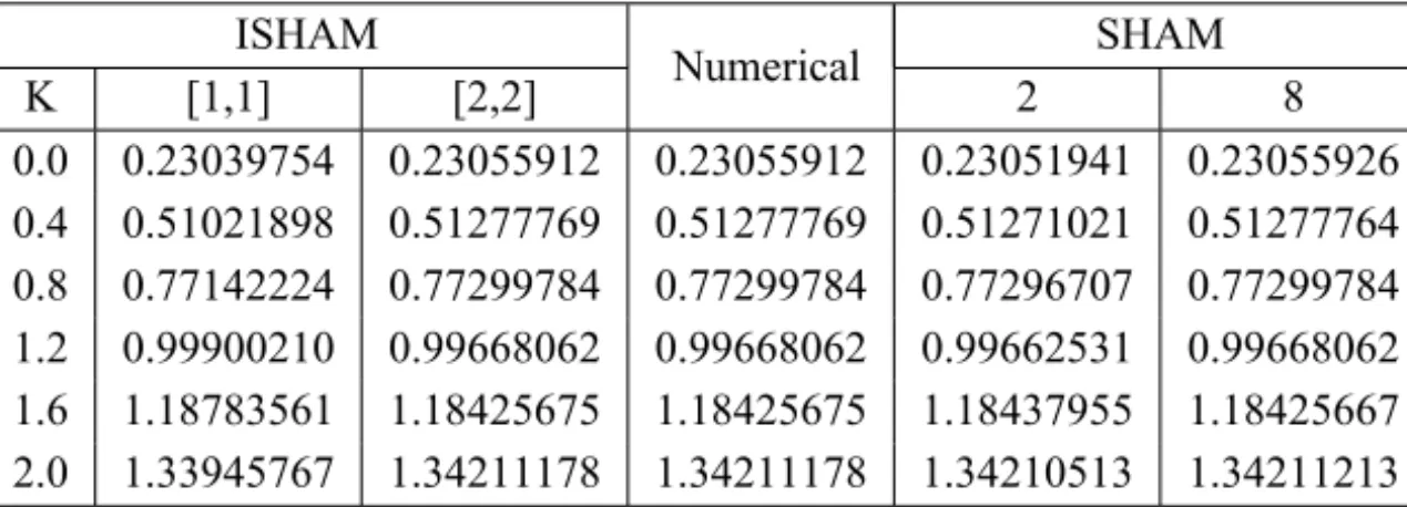
The radial shear stress whenM₌2 and for different values ofK is presented in Table 3. For validation of the current method, and to determine the effect of improving the initial guesses, we compare the results against the numerical solution. For convergence of the method the results are compared with the ‘standard’ spectral homotopy analysis method for the same values ofN,L and

~_{. For 0 ≤ K ≤ 2 the ISHAM converges at 2}nd_{order while the SHAM would}

in Table 4 where the absolute errors in the solution are given.

ISHAM SHAM

K [1,1] [2,2] Numerical 2 8

0.0 0.23039754 0.23055912 0.23055912 0.23051941 0.23055926 0.4 0.51021898 0.51277769 0.51277769 0.51271021 0.51277764 0.8 0.77142224 0.77299784 0.77299784 0.77296707 0.77299784 1.2 0.99900210 0.99668062 0.99668062 0.99662531 0.99668062 1.6 1.18783561 1.18425675 1.18425675 1.18437955 1.18425667 2.0 1.33945767 1.34211178 1.34211178 1.34210513 1.34211213

Table 3 – Radial shear stressF′(0): A comparison of the convergence rate of the ISHAM and SHAM to the numerical solutions for different values ofKwhenM₌2,Pr ₌1,Ec₌0.3.

ISHAM SHAM

K [1,1] [2,2] 2 8

0.0 0.00016158 0.00000000 0.00003971 0.00000014 0.4 0.00255871 0.00000000 0.00006748 0.0000005 0.8 0.0015756 0.00000000 0.00003077 0.00000000 1.2 0.00232148 0.00000000 0.00005531 0.00000000 1.6 0.00357886 0.00000000 0.00012280 0.00000008 2.0 0.00265411 0.00000000 0.00000665 0.00000035

Table 4 – Comparison of the absolute errors in the ISHAM and SHAM solutions for different values ofK whenM₌2,Pr₌1,Ec₌0.3.

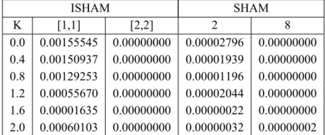
In Table 5, the tangential stress results obtained using the ISHAM and the SHAM are compared with the numerical results whenM ₌2 and for different values ofK. Convergence of the ISHAM to the numerical solutions was achieved at the 2nd _{order of approximation. When using the SHAM convergence to the} numerical solution was achieved at the 8th_{order for values ofKup to 2. It is also} clear that the ISHAM is computationally much more efficient compared to the SHAM. A comparison of the absolute errors is made in Table 6 where the fast convergence of the ISHAM when compared with the SHAM is confirmed. It is worth noting that the SHAM converges faster for₋G′_{(0) compared to F}′_(0). This is due to the differences in the level of nonlinearity of the equations ofF(η)

difference in the nonlinearity of functions. This there appears to be an added advantage of the ISHAM over the SHAM.

ISHAM SHAM

K [1,1] [2,2] Numerical 2 8

0.0 1.44053856 1.44209401 1.44209401 1.44206605 1.44209401

RT 0.1225 0.1125 0.2423 0.6168

0.4 1.49006904 1.49157841 1.49157841 1.49155902 1.49157841

RT 0.1214 0.1231 0.2589 0.6843

0.8 1.55193969 1.55323222 1.55323222 1.55322026 1.55323222

RT 0.1233 0.1121 0.2378 0.6819

1.2 1.62016082 1.62071752 1.62071752 1.62069708 1.62071752

RT 0.1199 0.1129 0.2626 0.6563

1.6 1.68975142 1.68973507 1.68973507 1.68973529 1.68973507

RT 0.1249 0.1192 0.2415 0.6850

2.0 1.75748201 1.75808304 1.75808304 1.75808336 1.75808306

RT 0.1264 0.1150 0.2484 0.6638

Table 5 – Comparison of the approximate solutions of₋G′(0)at different ISHAM and SHAM orders against the numerical solutions for different values ofKwhenM=2,Pr =1,Ec=0.3.

ISHAM SHAM

K [1,1] [2,2] 2 8

0.0 0.00155545 0.00000000 0.00002796 0.00000000 0.4 0.00150937 0.00000000 0.00001939 0.00000000 0.8 0.00129253 0.00000000 0.00001196 0.00000000 1.2 0.00055670 0.00000000 0.00002044 0.00000000 1.6 0.00001635 0.00000000 0.00000022 0.00000000 2.0 0.00060103 0.00000000 0.00000032 0.00000002

Table 6 – Comparison of the absolute errors in the ISHAM and SHAM solutions compared to the numerical solution for different values ofK whenM₌2,Pr₌1,Ec₌0.3.

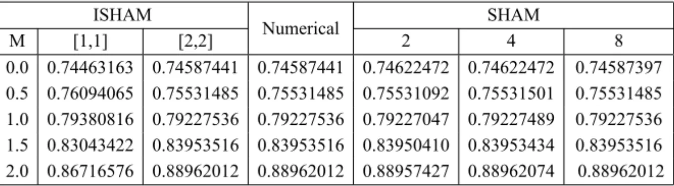
Table 7 gives a comparison of the convergence rate of the ISHAM and the SHAM versus the numerical solutions for F′(0) for different values M when

the numerical solutions for different valuesM whenK ₌1. An increase in the tangential shear stress is observed with an increase in M. The absolute errors are shown in Table 10. The nonlinearity of the equations has no effect on the convergence of the ISHAM.

ISHAM SHAM

M [1,1] [2,2] Numerical 2 4 8

0.0 0.74463163 0.74587441 0.74587441 0.74622472 0.74622472 0.74587397 0.5 0.76094065 0.75531485 0.75531485 0.75531092 0.75531501 0.75531485 1.0 0.79380816 0.79227536 0.79227536 0.79227047 0.79227489 0.79227536 1.5 0.83043422 0.83953516 0.83953516 0.83950410 0.83953434 0.83953516 2.0 0.86716576 0.88962012 0.88962012 0.88957427 0.88962074 0.88962012 Table 7 – Comparison of the approximate solutions of F′(0)at different_[i,m_] orders of the ISHAM, SHAM orders and against the numerical solutions for different values ofMwhenK₌1,

Pr=1,Ec=0.3.

ISHAM SHAM

M [1,1] [2,2] 2 4 8

0.0 0.00124279 0.00000000 0.00035031 0.00003159 0.00000044 0.5 0.00562580 0.00000000 0.00000393 0.00000016 0.0000000 1.0 0.00153280 0.00000000 0.00000489 0.00000047 0.00000000 1.5 0.00910094 0.00000000 0.00003106 0.00000082 0.00000000 2.0 0.02245436 0.00000000 0.00004585 0.00000062 0.00000000

Table 8 – Comparison of the absolute errors for the approximate solutions ofF′(0)at different [i,m_]orders of the ISHAM, SHAM orders and against the numerical solutions for different values ofMwhenK ₌1,Pr₌1,Ec₌0.3.

Table 11 shows the heat transfer coefficient−2′(0)at different orders of the ISHAM compared against numerical results for different values ofM, Pr, and

ISHAM SHAM

M [1,1] [2,2] Numerical 2 4 8

0.0 0.77672002 0.77834765 0.77834765 0.77854199 0.77836167 0.77834730 0.5 1.01294536 1.01069483 1.01069483 1.01070160 1.01069527 1.01069483 1.0 1.22319102 1.22367051 1.22367051 1.22366267 1.22367003 1.22367051 1.5 1.40999393 1.41449208 1.41449208 1.41447134 1.41449166 1.41449208 2.0 1.57840020 1.58657262 1.58657262 1.58655736 1.58657305 1.58657262 Table 9 – Comparison of the approximate solutions of₋G′(0)at different ISHAM and SHAM orders and against the numerical solutions for different values ofM when K ₌ 1, Pr ₌ 1,

Ec=0.3.

ISHAM SHAM

M [1,1] [2,2] 2 4 8

0.0 0.00162763 0.00000000 0.00019434 0.00001402 0.00000035 0.5 0.00225053 0.00000000 0.00000677 0.00000044 0.0000000 1.0 0.00047949 0.00000000 0.00000784 0.00000048 0.00000000 1.5 0.00449815 0.00000000 0.00002074 0.00000042 0.00000000 2.0 0.00817242 0.00000000 0.00001526 0.00000043 0.00000000 Table 10 – Comparison of the absolute errors for the approximate solutions of₋G′(0)at differ-ent ISHAM and SHAM orders and against the numerical solution for differdiffer-ent values ofMwhen

K ₌1,Pr₌1,Ec₌0.3.

M Pr Ec [1,1] [2,2] [3,3] [4,4] Numerical

0 0.33894036 0.33798332 0.33798332 0.33798332 0.33798332 0.5 1 0.3 0.18638822 0.18165630 0.18165630 0.18165630 0.18165630 1.0 0.07138752 0.05317238 0.05317238 0.05317238 0.05317238 1.5 –0.01803593 –0.05185078 –0.05185078 –0.05185078 –0.05185078 3 0.13954354 0.13959137 0.13959137 0.13959137 0.13959137 0.5 5 0.3 0.00576310 0.00730445 0.00730445 0.00730445 0.00730445 7 –0.15265228 –0.15060972 –0.15060972 –0.15060972 –0.15060972 10 –0.40767193 –0.40565482 –0.40565482 –0.40565482 –0.40565482 1 –0.32997005 –0.33670269 –0.33670269 –0.33670269 –0.33670269 0.5 1 3 –1.80527938 –1.81772838 –1.81772838 –1.81772838 –1.81772838 6 –4.01824339 –4.03926691 –4.03926691 –4.03926691 –4.03926691 9 –6.23120739 –6.26080545 –6.26080545 –6.26080545 –6.26080545

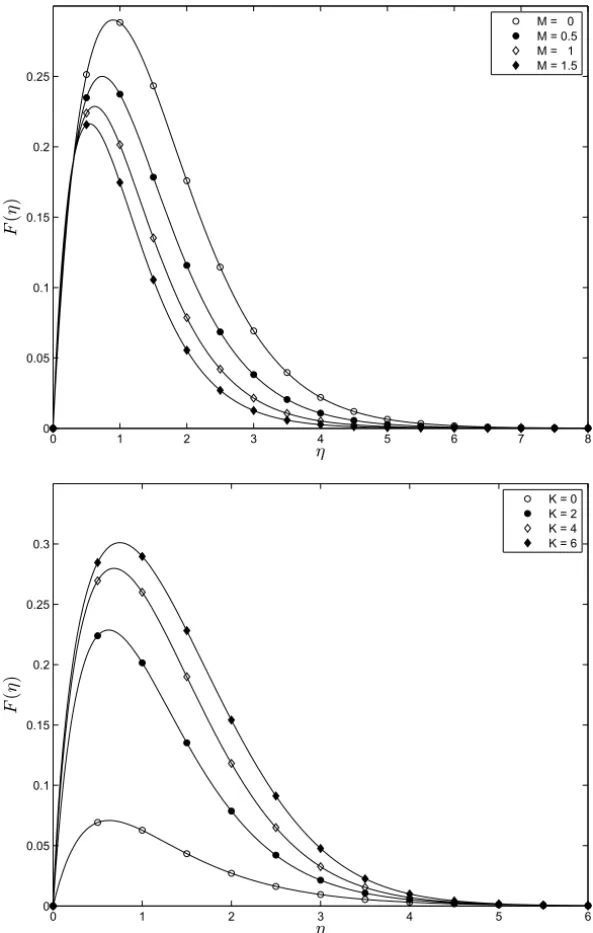
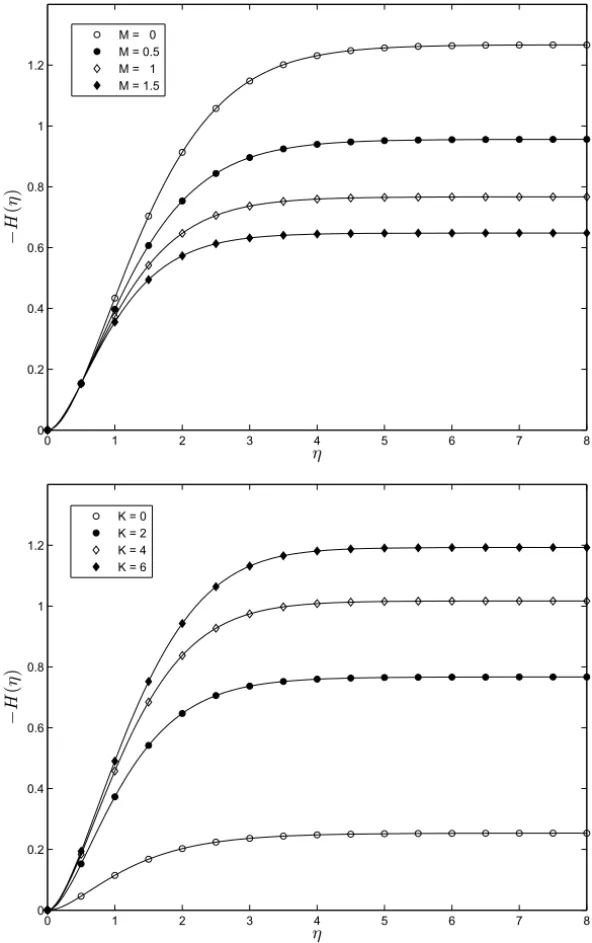
Figures 1-2 show the effect of MandK on the radial and axial velocity pro-files respectively. Increasing M reduces the radial component of the velocity while increasing K enhances F. The axial velocity H(η) increases with the magnetic parameter but decreases whenK is increased. There is excellent agree-ment between the second order ISHAM solutions for F(η)and H(η)and the numerical result.

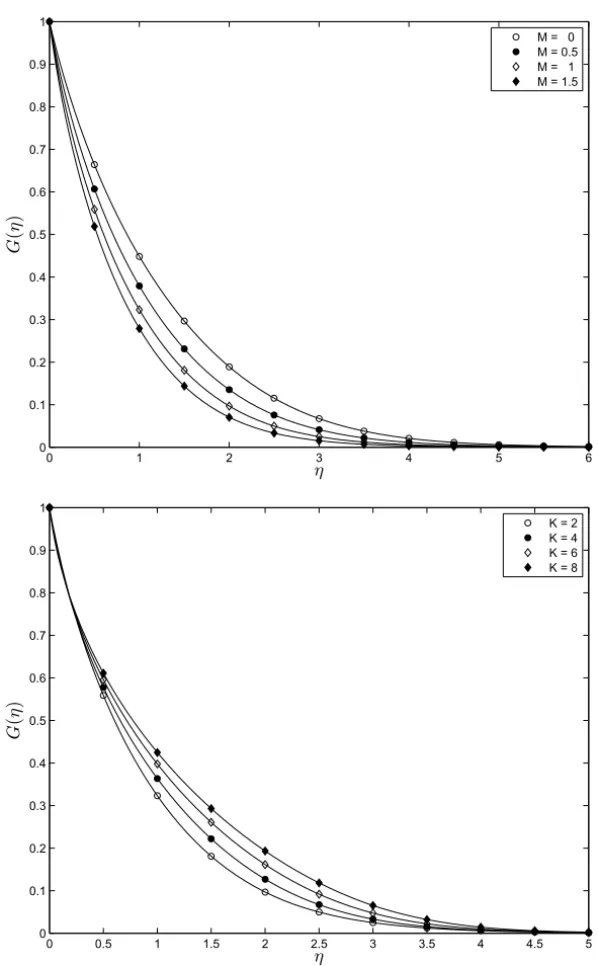
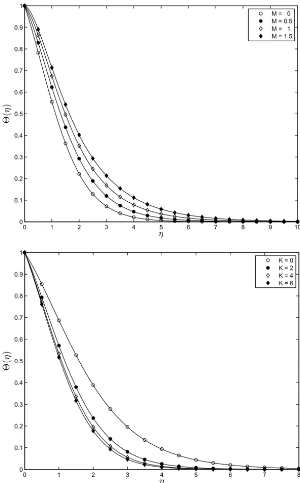
The tangential velocity component and the temperature profiles are show in Figures 3-4 for different values of M and K respectively. An increase in M

reduces G(η) while enhancing the 2(η). When K values are increased both

G(η)and2(η)decrease.

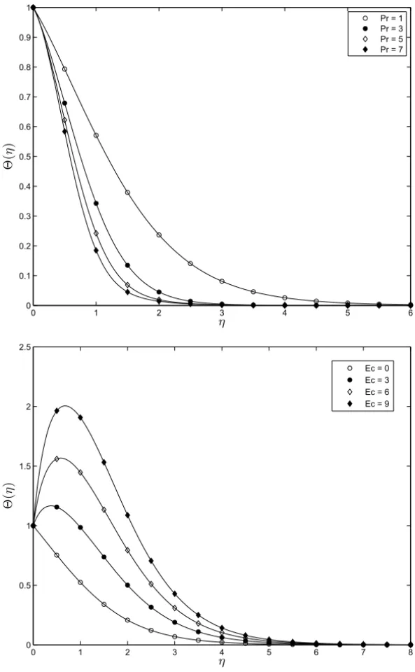
In Figure 5 temperature profiles are presented for varying values of Pr

and Ec. The temperature decreases with increasing Prandtl numbers while an increase in the Eckert number enhances the temperature.

6 Conclusion

A novel approach for accelerating the convergence of the spectral homotopy analysis method that is used to solve nonlinear equations in science and engi-neering has been proposed and applied successfully to the nonlinear system of equations governing the Reiner-Rivlin fluid in with Joule heating and viscous dissipation. The primary objective of the algorithm is to improve the initial approximate solution. The improved approximations are then used in the algo-rithm of the spectral-homotopy analysis method to reduce the number of itera-tions required to achieve convergence and better accuracy. The shear stresses in the radial and azimuthal directions were computed and the corresponding abso-lute errors determined. Convergence to the numerical solutions of the ISHAM approximate solutions was achieved at the 2nd orders for all flow parameters while the SHAM converged at the 8th_{order for some of the flow parameters.}

0 1 2 3 4 5 6 7 8 0

0.05 0.1 0.15 0.2 0.25

η

F

(

η

)

M = 0 M = 0.5 M = 1 M = 1.5

0 1 2 3 4 5 6

0 0.05 0.1 0.15 0.2 0.25 0.3

η

F

(

η

)

K = 0 K = 2 K = 4 K = 6

Figure 1 – On the comparison between the 2ndorder ISHAM solution and the numer-ical solution (solid line) for F(η)at different values of M (K = 2)andK (M =1)

0 1 2 3 4 5 6 7 8 0

0.2 0.4 0.6 0.8 1 1.2

η

−

H

(

η

)

M = 0 M = 0.5 M = 1 M = 1.5

0 1 2 3 4 5 6 7 8

0 0.2 0.4 0.6 0.8 1 1.2

η

−

H

(

η

)

K = 0 K = 2 K = 4 K = 6

Figure 2 – On the comparison between the 2ndorder ISHAM solution and the numer-ical solution (solid line) for−H(η)at different values of M(K =2)andK (M =1)

0 1 2 3 4 5 6 0

0.1 0.2 0.3 0.4 0.5 0.6 0.7 0.8 0.9 1

η

G

(

η

)

M = 0 M = 0.5 M = 1 M = 1.5

0 0.5 1 1.5 2 2.5 3 3.5 4 4.5 5 0

0.1 0.2 0.3 0.4 0.5 0.6 0.7 0.8 0.9 1

η

G

(

η

)

K = 2 K = 4 K = 6 K = 8

Figure 3 – On the comparison between the 2ndorder ISHAM solution (figures) and the bvp4c numerical solution (solid line) forG(η)at different values of M (K =2)and

0 1 2 3 4 5 6 7 8 9 10 0

0.1 0.2 0.3 0.4 0.5 0.6 0.7 0.8 0.9 1

η

Θ

(

η

)

M = 0 M = 0.5 M = 1 M = 1.5

0 1 2 3 4 5 6 7 8

0 0.1 0.2 0.3 0.4 0.5 0.6 0.7 0.8 0.9 1

η

Θ

(

η

)

K = 0 K = 2 K = 4 K = 6

Figure 4 – On the comparison between the 2ndorder ISHAM solution (figures) and the bvp4c numerical solution (solid line) for2(η)at different values of M (K =2)and

0 1 2 3 4 5 6 0

0.1 0.2 0.3 0.4 0.5 0.6 0.7 0.8 0.9 1

η

Θ

(

η

)

Pr = 1 Pr = 3 Pr = 5 Pr = 7

0 1 2 3 4 5 6 7 8

0 0.5 1 1.5 2 2.5

η

Θ

(

η

)

Ec = 0 Ec = 3 Ec = 6 Ec = 9

Figure 5 – On the comparison between the 2nd_{order ISHAM solution (figures) and the}

bvp4c numerical solution (solid line) for2(η)at different values ofPr(Ec=0.3)and

The effect of K andM was determined and it was observed that an increase in K results in an increase in F(η), and a decrease in H(η), G(η) and2(η)

while increasing M increases H(η)and2(η) while both F(η)and G(η) de-creases. 2(η) decreased with an increase in the Ec and decreased with an increase inPr. The success of the ISHAM in solving the non-linear equations governing the von Kármán flow of an electrically conducting non-Newtonian Reiner-Rivlin fluid in the presence of viscous dissipation, Joule heating and heat transfer proves that the ISHAM fits as a newly improved method of solution that can be used to solve non-linear problems arising in science and engineering.

Acknowledgements. The authors wish to acknowledge financial support from the University of KwaZulu-Natal and the National Research Foundation (NRF).

REFERENCES

[1] M.A. Abdou,New Analytical Solution of Von Karman swirling viscous flow. Acta. Appl. Math.,111(2010), 7–13.

[2] P.D. Ariel,The homotopy perturbation method and analytical solution of the prob-lem of flow past a rotating disk. Computers and Mathematics with Applications, 58(2009), 2504–2513.

[3] A. Arikoglu, I. Ozkol and G. Komurgoz,Effect of slip on entropy generation in a single rotating disk in MHD flow. Applied Energy,85(2008), 1225–1236.

[4] H.A. Attia,The effect of ion slip on the flow of Reiner-Rivlin fluid due to a rotating disk with heat transfer. J. of Mechanical Science and Technology, 21 (2007), 174–183.

[5] H.A. Attia, Rotating disk flow and heat transfer through a porous medium of a non-Newtonian fluid with suction and injection. Communications in Nonlinear Science and Numerical Simulation,13(2008), 1571–1580.

[6] H.A. Attia and M.E.S. Ahmed, Non-Newtonian conducting fluid flow and heat transfer due to a ratating disk. ANZIAM Journal,46(2004), 237–248.

[7] H.A. Attia,Ion-slip effect on the flow due to a rotating disk. The Arabian J. for Sc. and Eng.,29(2004), 165–172.

[9] H.A. Attia,Steady Flow over a Rotating Disk in Porous Medium with Heat Trans-fer. Nonlinear Analysis: Modelling and Control,14(2009), 21–26.

[10] H.A. Attia, Rotating disk flow with heat transfer of a non-Newtonian fluid in porous medium. Turk. J. Phys.,30(2006), 103–108.

[11] H.A. Attia,On the effectiveness of uniform suction and injection on steady rotating disk flow in porous medium with heat transfer. Turkish J. Eng. Env. Sci.,30(2006), 231–236.

[12] E.R. Benton,On the flow due to a rotating disk. J. Fluid Mech.,24(1966), 781–800.

[13] C. Canuto, M.Y. Hussaini, A. Quarteroni and T.A. Zang,Spectral Methods in Fluid Dynamics, Springer-Verlag, Berlin (1988).

[14] C.S. Chien and Y.T. Shih, A cubic Hermite finite element-continuation method for numerical solutions of the von Kármán equations. Appl. Math. and Comp., 209(2009), 356–368.

[15] W.G. Cochran,The flow due to a rotating disk. Math. Proc. Cambridge Philos. Soc.,30(1934), 365–375.

[16] W.S. Don and A. Solomonoff,Accuracy and speed in computing the Chebyshev Collocation Derivative. SIAM J. Sci. Comput.,16(1995), 1253–1268.

[17] A. El-Nahhas, Analytic approximations for von Kármán swirling flow. Proc. Pakistan Acad. Sci.,44(3) (2007), 181–187.

[18] P. Hatzikonstantinou,Magnetic and viscous effects on a liquid metal flow due to a rotating disk. Astrophysics and Space Science,161(1989), 17–25.

[19] N. Kelson and A. Desseaux,Note on porous rotating disk flow. ANZIAM Journal, 42(E) (2000), C837–C855.

[20] S.J. Liao, Beyond perturbation: Introduction to homotopy analysis method. Chapman & Hall/CRC Press (2003).

[21] Z.G Makukula, P. Sibanda and S.S. Motsa,On new solutions for heat transfer in a visco-elastic fluid between parallel plates, International journal of mathematical models and methods in applied sciences,4(4) (2010), 221–230.

[22] Z.G Makukula, P. Sibanda and S.S. Motsa, A Novel Numerical Technique for Two-Dimensional Laminar Flow between Two Moving Porous Walls, Mathemat-ical Problems in Engineering, 2010 (2010), Article ID 528956, 15 pages doi: 10.1155/2010/528956.

[24] M. Miklav˜ci˜c and C.Y. Wang,The flow due to a rough rotating disk. Z. Angew. Math. Phys.,54(2004), 1–12.

[25] S.S. Motsa, P. Sibanda and S. Shateyi,A new spectral-homotopy analysis method for solving a nonlinear second order BVP, Communications in Nonlinear Science and Numerical Simulation,15(2010), 2293–2302.

[26] S.S. Motsa, P. Sibanda, F.G. Awad and S. Shateyi,A new spectral-homotopy ana-lysis method for the MHD Jeffery-Hamel problem. Computers & Fluids,39(2010), 1219–1225.

[27] S.S. Motsa and P. Sibanda,On the solution of MHD flow over a nonlinear stretch-ing sheet by an efficient semi-analytical technique. Int. J. Numer. Meth. Fluids, (2011), doi: 10.1002/fld.

[28] S.S. Motsa, G.T. Marewo, P. Sibanda and S. Shateyi,An improved spectral ho-motopy analysis method for solving boundary layer problems. Boundary Value Problems,3(2011), doi: 10.1186/1687-2770-2011-3, 11 pages.

[29] E. Osalusi, Effects of thermal radiation on MHD and slip flow over a porous rotating disk with variable properties. Romanian Journal Physics, 52 (2007), 217–229.

[30] E. Osalusi and P. Sibanda,On variable laminar convective flow properties due to a porous rotating disk in a magnetic field. Romanian Journal Physics,51(2006), 937–950.

[31] M.M. Rashidi and S.A.M. Pour,A novel analytical solution of steady flow over a rotating disk in porous medium with heat transfer by DTM-padé. African J. of Math. and Comp. Sc. Research,3(2010), 93–100.

[32] M.M. Rashidi and H. Shahmohamadi, Analytical solution of three-dimensional Navier-Stokes equations for the flow near an infinite rotating disk. Communica-tions in Nonlinear Science and Numerical Simulation,14(2009), 2999–3006.

[33] B. Sahoo,Effects of partial slip, viscous dissipation and Joule heating on von Kármán flow and heat transfer of an electrically conducting non-Newtonian fluid. Communications in Nonlinear Science and Numerical Simulation, 14 (2009), 2982–2998.

[34] B.K. Sharma, A.K. Jha and R.C. Chaudhary,MHD forced flow of a conducting viscous fluid through a porous medium induced by an impervious rotating disk. Rom. Journ. Phys.,52(2007), 73–84.

[36] L.N. Trefethen,Spectral Methods in MATLAB. SIAM (2000).

[37] M. Turkyilmazoglu,Purely analytic solutions of magnetohydrodynamic swirling boundary layer flow over a porous rotating disk. Computers & Fluids,39(2010), 793–799.

[38] M. Turkyilmazoglu,Purely analytic solutions of the compressible boundary layer flow due to a porous rotating disk with heat transfer. Physics of fluids,21(2009), 106104–12.

[39] T. von Kármán, Uberlaminare und turbulence reibung. ZAMM,1(1921), 233– 252.

[40] C. Yang and S.J. Liao, On the explicit, purely analytic solution of von