Revista Árvore, Viçosa-MG, v.40, n.6, p.1119-1130, 2016
CREEP IN THE FUNDAMENTAL FREQUENCY AND STABILITY OF A
SLENDER WOODEN COLUMN OF COMPOSITE SECTION
1Alexandre de Macêdo Wahrhaftig2*, Reyolando Manoel Lopes Rebello da Fonseca Brasil3 and Sandro Fábio César2
1 Received on 07.05.2015 accepted for publication on 16.09.2016.
2 Universidade Federal da Bahia, Escola Politécnica, Departamento de Construções e Estruturas, Salvador, Bahia - Brasil.
E-mail: <alixa@ufba.br> and <sfcesarpaz@uol.com.br>.
3 Universidade Federal do ABC, Centro de Engenharia, Modelagem e Ciências Sociais Aplicadas, Santo André, São Paulo
-Brasil. E-mail: <reyolando.brasil@ufabc.edu.br>. *Corresponding author.
ABSTRACT – Creep is a phenomenon that can occur in wooden structures since wood is a viscoelastic material. Creep may change the purely elastic parameters determined in wood characterization initial tests, as its behavior depends on the rheology of the material, even under a constant stress level. Mathematically, creep can be characterized by models in which the immediate elastic deformation is increased by a viscous deformation, resulting in a temporal function. For this reason, the calculation of the natural frequency of vibration and the stability verification of a slender column should include the reducing effects of stiffness both of axial force and creep. The first one can be considered through the geometrical portion and the second one by the introduction, in the conventional portion, of a variable elasticity modulus over time, obtained in relation to the adopted rheological model. A numerical simulation was performed to evaluate the aspects above, considering a bar compressed by a force at the free end equivalent to 10% of the Euler critical force, plus its own weight, adopting a rheological model with three parameters for the variation of the elasticity modulus. The results show differences of 60% and 50% for the frequency and elasticity modulus, besides defining the exact instant of column collapse in the case of its non-observance.
Keywords: Three-parameter model; Vibration; Stability.
A FLUÊNCIA NA FREQUÊNCIA FUNDAMENTAL E NA ESTABILIDADE DE
UMA COLUNA ESBELTA DE MADEIRA DE SEÇÃO COMPOSTA
RESUMO – A fluência é um fenômeno que pode ocorrer em estruturas de madeira por ser esse um material viscoelástico. A fluência pode alterar os parâmetros puramente elásticos determinados nos ensaios iniciais de caracterização da madeira, pois o seu comportamento depende da reologia do material, mesmo com um nível de tensão constante. Matematicamente, a fluência pode ser caracterizada por modelos onde a deformação elástica imediata é acrescida de uma deformação viscosa, resultando em uma função temporal. Por essa razão, o cálculo da frequência natural de vibração e a verificação da estabilidade de uma coluna esbelta devem incluir os efeitos redutores da rigidez tanto da força axial quanto da fluência. O primeiro pode ser considerado por meio da parcela geométrica e o segundo pela introdução, na parcela convencional, de um módulo de elasticidade variável com o tempo, obtido em relação ao modelo reológico adotado. Para avaliar os aspectos mencionados, foi realizada uma simulação numérica, considerando uma peça comprimida por uma força na extremidade livre equivalente a 10% da força crítica de Euler, mais o seu peso próprio, adotando-se um modelo reológico de três parâmetros para a variação do módulo de elasticidade. Os resultados indicaram diferenças de 60% e 50% para a frequência e para o módulo de elasticidade, além de definir o instante exato de colapso da coluna em caso de sua inobservância.
1. INTRODUCTION
The slow increase of deformation under constant stress over time is called creep. Mathematically, creep can be represented by a time-dependent function associated with viscoelastic rheological models capable of describing the phenomenon, according to Findley; Lai; Onaran (1989). The slow deformation, or creep, in wooden structures, is a time-dependent phenomenon, which is also related to loads and deformations, defined as the increase of deformation under the action of loads, or permanent stresses, over time. Creep produces residual deformation and can change the characteristics of the materials and their mechanical properties, and it is even able to produce the failure of a structure, as reported by Gottron; Harries; Xu (2014). When wooden structures are used as horizontal components and loaded, they undergo long-term deformation and, in different humidity conditions, the wood has a tendency to increase its deformation due to creep, which can lead to operational problems due to excessive deformation, or may cause safety problems due to loss of resistance, which can decrease the load capacity and, in the case of columns, reach the buckling stress, emphasize Epmeier; Johansson; Kliger; Westin (2007).
In general, two types of criteria are used to represent the creep within the structural design. The first one is related to a deformation limit value, restricting it to validity intervals, and the second one, less common, takes into account a monotonic growth of deformation. From a practical point of view, the technical standards take into account the creep phenomenon in the design of structures by two considerations: by proposing a coefficient of increase or decrease of stiffness, or proposing a coefficient of increase or decrease in resistance as the loading acting time and humidity class, according to Celia-Silva; Calil Junior (1992). The decrease in stiffness is related to the fact that the axial force is responsible for this effect and can lead to loss of stability of a column. In this sense, Gambhir (2004) refers to the influence of the compressive force highlighting that once there is a reduction in the structural stiffness, the effect of the loads on the structure increases, which also increases the forces on the elements, so the structure resistance capacity decreases. For this reason, in the case of compressed columns, a premature analysis can produce undesirable consequences, and any failure causes catastrophic effects since it involves the balance of structures, Timoshenko (1992).
includes the three directions of wood orthotropy was developed in the sixties of the twentieth century (BHATNAGAI; GUPTA, 1967).
Because of its plastic behavior, even with a constant level of tension, the deformations in structural elements of wood tend to increase with time, i.e. after the initial elastic deformations, additional deformations occur, which can be reversible or not, but never complete. The slow creep is partially reversible. For an unloading, after elastic recovery, there is a later recovery, which is called slow recoverable deformation, slow reversible deformation, or delayed elastic deformation, and only a remaining portion of the deformation is residual or irreversible, being this portion of deformation called creep, Leohard; Mong (1977).
In Brazil, there are some records of studies regarding creep on wooden structures carried out by Almeida (1990) and Celia-Silva; Calil Junior (1992). The studies conducted by the first researcher, on tensioned parts, revealed high levels of creep after the first twenty-four hours of the assay, corresponding to a rapid creep phenomenon, and a convergence after 90 days. The measurements were made daily and involved the recording of deformations and environmental conditions (temperature and relative air humidity). On the other hand, the second researchers conducted experiments on slow deformation in wooden columns. Their studies evidenced a tendency for creep stability after 60 and 90 days of loading. Studies on creep in wood, considering it under several aspects, were more recently developed by George et al. (2003), Wang, J.B.; Foschi, R.O.; Lam, F (2012;2012), Reynolds, T.; Harris, R.; Chang, Wen-Shao (2013), Honfi,D. et al. (2014), Sharapov, E.; Mahnert, K.C; Militz, H. (2016) and Saifouni et al. (2016).
Commonly, the representation of creep is based on rheological models, which associate deformations deferred at the time. These models, according to Gomes et al (2007), allow to simulate the response of the material to forces and tensions applied to it. The inclusion of these rheological models can be made both in static analysis and dynamic of the structures. In the case of dynamic analysis, the structure stiffness must be composed of two terms; the first one corresponding to the portion of conventional stiffness and the second to the portion of geometric stiffness, according to Clough; Penzien (1993). Thus, it is possible to adapt the first portion of stiffness by introducing a variable elasticity
modulus over time, making possible to monitor the increase of deformations, according to the adopted rheological model, keeping a constant stress level. Therefore, the total stiffness assumes the form introduced by the first portion, via elasticity modulus, in the rheological model intended to represent the creep; and the second portion is geometrical, which is a function of normal operating force, which includes the own weight of the structural element.
A numerical simulation was performed to evaluate the creep in natural frequency and in the stability of a slender wood column, taking into account a three-parameter model to represent its viscoelastic behavior. The formulation developed to calculate the column natural frequency of vibration was based on the method of virtual works and allowed the evaluation of the buckling critical load and loss of system instability, besides calculating the frequency of the first mode. The results indicated significant differences in the fundamental frequency and elastic modulus, considering values obtained by a purely elastic analysis and those non-linear with the creep, in relation to the material, and geometric value considering the geometric stiffness. It was also possible to define the exact moment of the column collapse in the case of non-observance of creep, considering a force of 10% of the critical load of Euler concentrated at the free end of the structural element. Comparison with design criteria and verification for parts in flexo-compression and stability of the NBR 7190 - Wooden Structures Design (1996) were adopted for this level of loading, as well as the definition of the limit percentage of the Euler critical load, which leads the system to the collapse, using these same criteria and mathematical tools developed in the present study.
2. MATERIAL AND METHODS 2.1 Mathematical simulation support
more suitable for the description of certain solids. The model of Group II (Figure 1b) describes the behavior of liquids simulating an initial viscous outflow and a slow elastic deformation over time. The model of Group III (Figure 1c) shows an instantaneous elastic response followed by a viscous response with a slow deformation as well. The model of Group IV (Figure 1d) simultaneously presents two slow viscous deformations over time. These models can be used alone or in associations, forming chains, in an attempt to obtain the best representation for each situation.
One of the models more used to represent the creep in several materials is the three-parameter model, in which an elastic parameter E0 is associated with a viscoelastic model of parameters E1 and 1 called Kelvin-Voigt model, which is a simplification of the Burgers model of Group type I (Figure 1a). According to Keramat; Shirazi (2014), a single model of the Kelvin-Voigt is enough to describe the viscoelastic nature of many solid. Based on this consideration an adaptation of the Burgers model was used by Kränkel; Lowke; Gehlen (2015) to analyze the non-linear viscoelastic deformation in bonded anchors. In relation to the wood, Mukudai (1983) mentions that the functional form represented by the Voigt and Maxwell models is very efficient since they can be conveniently applied to assess the viscoelastic behavior of that material through mathematical models. In this sense Hering; Niemz (2012)
have used the Kelvin-Voigt model, together with experimental activity to descript the creep in bended pieces. A Burger chain of four elements was used by Gao; Wang; Shao (2016) to study the behavior of Xuan paper, making possible to description convenientily the elastic, viscoelastic and plastic deformations presented by the material.
The adoption of Kelvin-Voigt model has repeatedly been made to study phenomena in various science fields. Hackney; Aifantis; Tangtrakarn; Shrivastava (2012) used this model to examine the creep behavior of nanostructures of composites. In the context of the finite element method, Chung; Tamma; Namburu (2000) used the Kelvin-Voigt model to represent the primary creep to investigated the thermo-viscoelastic of composite structures. Puertas; Gallego (2014) used the same model, together with the boundary element method, to consider the viscoelasticity in the solution of the three-dimensional dynamic problems.
Mathematically, the total deformation of the Kelvin-Voigt model is given by equation (1),
= e + v,
where ee is the deformation in the elastic model and ev is the deformation in the plastic model. Take into account its derivative relative to time, the total deformation of the model is found by equation (2),
(a) Kelvin-Voigt viscoelastic model of three
parameters – Group I (b) Kelvin-Voigt viscoelastic model of three parameters – Group II
(c) Burges viscoelastic model of four parameters –
Group III (d) Viscoelastic model of four parameters – Group IV
eElastic
Ec0ef
1
vViscoelastic
Ec0ef
vViscous
1
vViscoelastic
Ec0ef
1
Ec0ef
1 1
Ec0ef
eElastic vViscoelastic
v
Viscous
1
vViscoelastic
Ec0ef 1
Ec0ef
Figura 1 – Viscoelastic rheological models.
Figura 1 – Modelo reológicos viscoelásticos.
which is the constitutive equation of the Kelvin-Voigt model.
= e + v
The equation (3), for this specific case, is obtained by assuming E0 = E1 =
E
c ef0 , = Ec0efe and Ec0efv + 1v.
From the previous equations, it is obtained the differential equation (4) for the Kelvin-Voigt model, with t representing the moment of load application.
+ = Ec0ef +
As the stress is constant, the derivative of stress relative to time is null. By applying the above stress conditions, the equation (4) is reduced to equation (5), which is an ordinary differential equation,
whose general solution, for t > 0, with the initial condition (0) = is given by equation (6).
Obviously, if the stress level remains constant, the elasticity modulus must simultaneously reduce to as the deformation increases, then:
After finding the variable elasticity modulus over time, it is necessary to establish the conditions for an analysis of vibrations that, from the point of view of structural dynamics, make possible the obtainment of the temporal variation of the system natural frequency. One of the classic methods is the Modal Analysis. This method allows the obtainment of information about the behavior of a structural system and therefore reveals
important aspects related to its dynamics, such as frequencies and natural modes of vibration, according to Carrion; Mesquita; Ansoni (2014). In addition, it is possible to verify the stability of a structural system and the moment of its collapse, based on the nullability conditions of the fundamental frequency and, consequently, its stiffness.
The formulation developed in this simulation to consider the creep in the vibration of a column is based on the principle of virtual works associated with the Rayleigh technique, which suggests that for a system containing infinite degrees of freedom can be associated with another system with a single degree of freedom to bring its frequency closer, as described by Leissa (2004). The process takes into account the suitable choice of the generalized coordinate that describes the structure deformation, considering the first vibration mode. In the end, the equation of motion appears regarding the generalized system properties such as stiffness and mass, which are necessary to calculate the frequency. It is important to note that the technique developed by Rayleigh aimed to calculate the fundamental frequency of vibration of elastic systems, and the precision obtained by this method depends directly on the function chosen to represent this vibration mode, as also said by Leissa (2004).
The basic concept of the method is the principle of conservation of energy, and can, therefore, apply to linear structures (or not), according to Clough; Penzien (1993). Temple; Bickley (1933) consider that the Rayleigh technique is applied both to systems with infinite degrees of freedom and continuous systems, and serves both to determine the fundamental period of vibration and to verify the stability of mechanical systems, but it is not limited to these purposes. As seen in studies carried out by Villasenor; Farfán; Guzmánb; Romero; Castellanos; Sesma (2014), the Rayleigh technique was used in the detection of subsurface cracks in solids. Pena (2015) studied the asymmetric vibration of rigid bodies, considering the damping of Rayleigh in the context of small rotations, allowing the mathematical simplification of the problem. Cámara and Astiz (2014) used the form function technique as recommended by Rayleigh in the dynamic modal analysis of cable-stayed bridges, within the region of elastic deformation of the material.
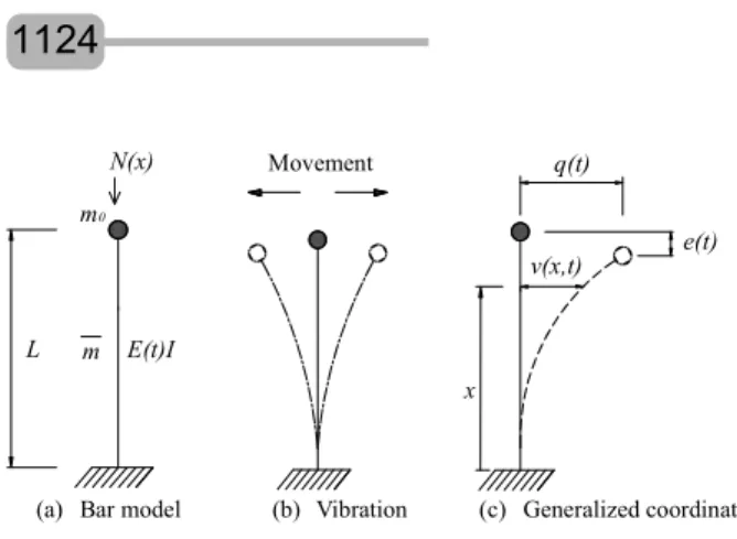
It is considered the model of the bar in Figure 2, of length L, in a free motion non-damping free motion,
Ec0ef + Ec0ef
1 Ec0ef 1Ec0ef
where 0, for t < 0
for t > 0
Ec0ef
(2)
(3)
(4)
(6)
(7)
Ec0ef + Ec0ef Ec0ef
1 (5)
1
with the generalized coordinate q(t) defined on the upper end of the element. The function v(x,t) provides the horizontal displacements for each x position along the height, in relation to a function (x) that describes the form of the vibration and meets the boundary conditions of the problem. It is assumed this system is composed of a prismatic bar, made of a viscoelastic material, clamped on its the base, supporting, in addition to its own weight m, a mass m0 at the free end, representative of bodies fixed to its top. N(x) is the normal generalized force and e(t) is the vertical displacement of the bar.
It is also considered that the system motion does not change the direction of the normal force. Thus, the represented structure is a bar in bending, so that the virtual work of internal forces WI is performed by the bending moment M(x,t), acting on the deflection of the virtual bar. It is assumed that the section remains flat after deformation. The Principle of Virtual Works requires that the virtual work of external forces is equal to the virtual work of the internal forces. The virtual work of the external forces is obtained by equation (8),
in which the is fI (x) = m1(x) v(x,t) the inertial force. In turn, the virtual work of the internal forces is given by equation (9).
An infinitesimal element ds of the curved bar is required to find the axial displacement e(t). The shortening of the axis due to the axial displacement is given by equation (10).
From the binomial development, considering that the higher order terms are smaller compared to the first order term, the initial series can be reduced, as observed in equation (11).
The reduction of the series by the binomial development allows rewriting equation (10) into a more compact form, as shown in equation (12).
The total displacement e(t) throughout the column comes from the integration of equation (12), as indicated in equation (13) in which the first derivative of that function is represented by an upper row to the right.
The real and virtual displacements and their derivatives, with the same notation established in equation (13), which are expressed in function of the generalized coordinate and the chosen shape function to represent the considered vibration mode, are calculated by equation (14).
Appropriately substituting the equations (13) and (14) in the equations (8) and (9), the equations (15) and (16) are obtained.
By equating the expressions (15) and (16) and adjusting the terms, the equation of the free undamped (b) Vibration
(a) Bar model E(t)I m N(x) m0 L Movement
(c) Generalized coordinate v(x,t)
x
q(t)
e(t)
Figure 2 – Mathematical model.
Figura 2 – Modelo matemático.
0
( ) ( ) ( ) ,
L E I
W f x v x dx N x e
2 2 0
( )
( , ) ( ) , com ( ) .
L
I v x
W M x t v x dx v x x
2 4 6 2
1 1
2 2 2 2
1 1 1 1 ,
2 8 16 2
dv dv dv dv
dv dx dx dx dv dx
dx dx 2 2 1 1 1 . 2 2 dv dv
ds dx dx dx
dx dx
20 1
( ) ( , ) .
2 L
e t
v x t dx0
( , ) ( ) ( ); ( , ) ( ) ( ); L ( , ) ( ) .
v x t x q t v x t x q t v x t x q t v x t x q t v x t x q t v x t x q t
v x t x q t v x t x q t e v x t v x dx
( ( ( ( ; ; ( ( ( ( ( ) ( ) ; ; , , , , ( ) ( ) ; ; ( ( ( ) ( )
2
21
0 0
( )L ( ) ( ) ( )L ( ) ( ) e
E
W q t m x x dx q t N x x dx q
2 0
( ) ( ) ( )L .
I
W q t E t I x dx q
motion appears regarding the generalized coordinate
q(t), as equation (17),
in which M, K0 and Kg are the generalized mass and the generalized conventional and geometric stiffness, described from the chosen form function . By assuming the trigonometric function to describe the vibratory motion, the generalized conventional stiffness is given by equation (18),
where E(t) is the variable modulus of elasticity with time, as shown in equation (7), and I is the inertia of the section in relation to the considered motion. The generalized geometric stiffness is calculated by equation (19),
in which N(x) = [m0 +m (L - x)]g is the normal force function, which includes the own weight of the column and the force concentrated at the free end. The generalized mass is obtained by equation (20),
where m0 is the mass concentrated at the top of the bar and m is the mass per unit length obtained by multiplying the section area by the density of the material. As the natural frequency depends directly on the total stiffness and inversely on the mass, it should be calculated by equation (21).
Therefore, the equation of the frequency of the first mode of vibration, in Hertz, which includes the geometric effect and creep, is finally provided by equation (22),
in which L is the length of the column, g is the gravity acceleration and E(t) the temporal elastic modulus as found in equation (7). In equation (22), it can be observed the conventional portion of the stiffness of the column to the left of the negative sign in the numerator, in which is included the variable elasticity modulus due to creep, and the stiffness geometric portion to the right of the same sign, in which it is considered the force concentrated at the free end of the column by mass m0 in addition to its own weight by the parameter
m, which is the mass distributed per unit length, both multiplied by the gravity acceleration. In the denominator is the generalized mass of the system, where there is a factor of 0.227 multiplying the product mL. This fact induces which buckling critical load of the column is seen decreased from this value, when the own weight of the structural element is introduced, which is in line with Timoshenko (1992) who predicted, in static analysis, that this factor would be of the order 1/3. By applying the equation (22), it is performed, using a single mathematical operation and at once, a non-linear material analysis, with the creep, and a geometric non-linear analysis, with the effect of the normal force, dispensing the use of computational tools or iterative calculations. It is worth mentioning that the equation (22) was comparatively evaluated by experimental activity, in physical laboratory, and by modeling using the finite element method - FEM, by Wahrhaftig; Brasil; Balthazar (2013), and again using the FEM by Wahrhaftig and Brasil (2016), studying the frequency of a real structure, considering for both studies, linear and isotropic elastic material, presenting excellent convergence of results in both cases.
2.2 Evaluated model problem
For this simulation, a composite section wooden column was idealized, with the parameters of interest shown in Table 1. The adopted gravity acceleration
g was 9.81 m/s2. The characteristic parallel resistance to fibers (fc0k) and the elastic modulus (Eco) were adopted considering class wood C-60. The effective elastic modulus and calculating the resistance of the material were defined according to the recommendations of NBR 7190/1996 - Wood Structural Design (1996), according to equation (23). The used weighting and modification coefficients were: Kmod1 = 0.7, Kmod2 = 1.0, Kmod3 = 0.8 and wc= 1.4, then:
0
( )
( ) ( )
g( ) 0,
Mq t K t q t K q t
(
x
)=1-cos
(
x 2L
)
2 2
0 2
0
( )
( )
L( )
d
x
,
K t
E t I
dx
dx
20
0
, with
L( )
,
M m m
m
m x dx
2
0
( )
( )
,
L
g
d x
K
N x
dx
dx
(17)
(18)
(19)
(20)
(21)
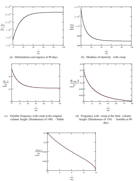
The numerical simulation was performed based on a column of height L and cross section as represented in Figure 3. The arrangement of the composite section was defined within a design reality typical of wooden structures and in function of the commercial limitations of laminated and glued wood, which had already been adopted in a design carried out by Wahrhaftig and Carvalho (2016). It is important to mention that the viscous parameter was adjusted so that the deformations stabilized at 90 days, as shown in Figure 4(a), as indicated by Almeida (1990), Celia-Silva; Calil Júnior (1992) and Kataoka; Bittencourt (2014). Thus, the variation of the elastic modulus
E(t) was obtained, represented by Figure 4 (b). It is emphasized the need to reduce the section inertia moment by multiplying it by a reduction factor of 0.7, since it is a composite section, constructed with screws, which is an important procedure to provide protection against plastic accommodation, specific of wooden connections, which was studied by Kharouf; Mcclure; Smith (2003) and Wilkinson; Rowland; Cooks (1981).
3. RESULTS
The column section was verified in relation to the flexocompression and stability according to the criteria of NBR 7190/1996 - Wooden Structures Design (1996), proving to be able, as the results presented in equation (24), in which KM = 0.5, and equation (25), respectively.
In equations (24) and (25), Nd, Md and fc0d are the calculation stresses due to the normal stress and bending moment, and calculation resistance to parallel compression to the fibers, obtained according to equations (26), with the results shown as MPa (106 Pa; Pa = N/ m2). The force concentrated at the free end of the bar, which induces the stresses Ncd and Md was established to represent one-tenth of the Euler force (FE) expected in equation (26)(c) where = 0.8, 1 = 0.6 and 2
= 0.4 are the creep coefficients appropriate to the case under study.
In equation (26) subindices c for N, E and mean compression; E in F is the buckling critical force of Euler; for e, the subindice i means initial, a accidental,
c creep; for w in g means weighting. Regarding the stress conditions in the design g and q in N, they indicate variable and permanent actions; k means characteristic, d for the design and ef effective value, calculated with the modification coefficients, shown in section 2.2.
Table 1 – Data of numerical simulation
Tabela 1 – Dados da simulação numérica.
Section data Column data
Inertia Area Length Slendernessl
I (cm4) A(cm2) L (m)
227812.50 1800 6.60 140
Rheological parameters Mass
Elasticity (MPa) Viscosity Density Lumped Per unity length
Ec0 (MPa) Ec0ef (MPa) (MPa*s) (kg/m3) m0(kg) m(kg/m)
24500 13720 32206086381.30 1100 51047.14 99
Figure 3 – Model of the structure.
Figura 3 – Modelo da estrutura.
(a) Column
(b) Section A -A – Dimensions in “cm”
(c) Composition of the cross section
L
A A m0
m = A
15 7,5 7,5 15
45
45
7,
515
15
7,
5
2
0 0 0
4
173.504 N
1, 0.964 ,
0.18
4851.07 0.45 0.684 0.964 0.684 0.50.684 0.07.
0.002 24 24 24
Ncd Md Md cd
M Ncd
c d c d c d d
Md
N
K MPa
f f f A m
M y Nm m MPa
I m
0 0
0.964 0.684
1, 0.06.
24 24
Md Md c d c d
f f
(23)
(24)
(a) Deformation convergence at 90 days (b) Modulus of elasticity with creep
(c) Variable frequency with creep at the original
column height (Slenderness of 140) - Stable (d)height (Slenderness of 156) – Instable at 90 Frequency with creep at the limit column days
(e) Structural collapse before 90 days (Slenderness of 156)
0 20 40 60 80 100
6105 8105 1104 1.2104 1.4104 1.6104
( )t 106
t day
0 20 40 60 80 100
6000 8000 1104 1.2104 1.4104
E t( ) MPa
t day
0 15 30 45 60 75 90 0
0.1 0.2 f L t()
Hz
t day
0 15 30 45 60 75 90 0
0.042 0.083 0.13 0.17 0.21 0.25
f Le90 t
Hz
t day
0 4 8 12 16
0 0.041 0.081 0.12 0.16
f 8m t( ) Hz
t day
Figure 4 – Results obtained by the numerical simulation.
Figura 4 – Resultados obtidos na simulação numérica.
4. DISCUSSION
The frequency of the column was then numerically calculated at the instants zero and 90 by equation (22),
as shown in Figure 4(c) and Figure 4(d). In the first case, the frequency variation was obtained by considering the original height of the column, adopted to obtain the limit slenderness established by the NBR 7190/1996 - Wooden Structures Design (1996). In the second case, the height of the column was designed to initiate its collapse at 90 days, defining thus the limit height it can have when the creep is introduced in the frequency calculation. In the first condition, the column is stable, whereas in the second case, the creep effect leads to loss of stability at the considered instant (90 days). Any height of the structure which
0
2 0
1 2
4851.07 , with 173504.051 , 123931.46 , 1.4,
2.796 , with 1239314.65 ,
d cd d cd ck wc
ck wc
c ef x E
d ef E
E cd b
M N e Nm N N N
N m g N
E I F
e e cm F N
F N L
1ef i a c, with i Mk= 0, a 300L = 2.2 , and
e e e e e e cm
N
1 21 2
1
( )exp 2.405 .
gk qk
E gk qk
ck
N N
F N N
c ig a
e e e cm
is defined between the stability limit at 90 days (second condition) and the limit established without creep, i.e., stability at instant zero (first condition), puts at risk the system equilibrium, which can be observed in Figure 4(e). For a height of 8 m, for example, the collapse would occur on the 16th day.
5. CONCLUSION
The elasticity modulus of 6865.265 MPa calculated by equation (7), at 90 days, represents a 50% decrease compared to the initial value of 13720 MPa. The structure frequency calculated at the initial time of loading is 0.262 Hz, and at 90 days is 0.106 Hz, representing a decrease of 60%. The column reaches its stability limit at the height of 7.35 m (slenderness of 156.19), collapsing at 90 days. Without considering the creep effect, the height limit is 10.37 m, at instant zero (slenderness of 220.41); a height of 29.14% higher than the previous one. This aspect is of great importance because, since if the height of the structure had been defined between the limit established without the creep and the limit determined considering the creep, the structure would collapse even before completing 90 days in service. For a height of 8 m (slenderness of 169.99), e.g., the collapse would occur close to the 16th day.
It can be concluded that the slenderness limit of 140, established by the Brazilian Standard, keeps the structure in safety condition regarding the loss of stability, considering a force 10% of the Euler force concentrated at the free end of the column. Additionally, it can be added that the safety limit condition is established by equation (24) for a critical load of 44.41% of the Euler Force at the end of the structure when it is simultaneously evaluated by equation (22).
6. REFERENCES
ALMEIDA, P.A.O. “Estruturas de Grande Porte de Madeira”. Tese (Doutorado em Engenharia Civil) - São Paulo: EPUSP, 1990.
ASSOCIAÇÃO BRASILEIRA DE NORMAS TÉCNICAS - ABNT — NBR 7190/1996. Projeto de Estruturas de Madeira. Rio de Janeiro: 1996.
BHATNAGAI, N.S.; GUPTA, R.P. “On the constitutive equations of the orthotropic theory of creep”. Wood Science and Technology, v.1, p.142-148, 1967.
BRÉMAUD I.; GRIL, J.; THIBAUT, B. Anisotropy of wood vibrational properties: dependence on grain angle and review of literature data. Wood Science
Technology, v.45, p.735-754, 2011.
CÁMARA, A.; ASTIZ, M.Á. “Aplicabilidad de las diversas estrategias de análisis sísmico en puentes atirantados en rango elástico”.
Revista Internacional de Métodos Numéricos para Cálculo y Diseño en Ingeniería, v.30, n.1, p.42-50, 2014.
CARRION, R.; MESQUITA, E.; ANSONI, J.L. “Dynamic response of a frame-foundation-soil system: a coupled BEM–FEM procedure and a GPU implementation”. Journal of the Brazilian Society of Mechanical Sciences and Engineering, v.37, n.4, p.1055–1063, 2014.
CELIA-SILVA, A.H.; CALIL JÚNIOR, C. Fluência da madeira. In: ENCONTRO BRASILEIRO EM MADEIRAS E EM ESTRUTURAS DE
MADEIRA, 1992, São Carlos. Anais... São Carlos: Lamem/Eesc-Usp, EESC - Escola de Engenharia de São Carlos, 1992.
CHUNG, P.W.; TAMMA, K.K.; NAMBURU, R.R. A finite element thermo-viscoelastic creep approach for heterogeneous structures with dissipative correctors. Finite Elements in Analysis and Design, v.36, p.279-313, 2000.
CLOUGH, R.W.; PENZIEN, J. Dynamic of structures. 2.ed. Taiwan: McGraw Hill International, 1993.
EPMEIER, H.; JOHANSSON, M.; KLIGER, R.; WESTIN, M., Bending creep performance of modified timber. Holz als Roh- und Werkstoff, v.65, p.343-351, 2007.
FINDLEY, W.N.; LAI, J.S.; ONARAN, K. Creep and relaxation of nonlinear
viscoelastic materials, whit an
introduction to linear viscoelasticity. New York: Dover Publications, 1989.
GAO, H.; WANG, F.; SHAO, Z. Study on the rheological model of Xuan paper, Wood Science Technology, v.50, p.427–440, 2016.
GEORGE, B.; SIMON, C.; PROPERZI, M.; PIZZI, A. Comparative creep characteristics of structural glulam wood adhesives. Holz als Roh- und Werkstoff, v.61, 79-80, 2003.
GOMES, E.A.S.; DANTAS NETO, A.A.; BARROS NETO, E.L.B.; LIMA, F.M.; SOARES, R.G.F.; NASCIMENTO, R.E.S., Aplicação de modelos
reológicos em sistemas: Parafina/Solvente/Tensoativo, 4º PDPETRO, 3.1.0197 – 1. Campinas: 2007.
GOTTRON, J.; HARRIES, K.A.; XU, Q. Creep behaviour of bamboo. Construction and Building Materials, v.66, p.79-88, 2014.
HACKNEY, S.A.; AIFANTIS, K.E.;
TANGTRAKARN, A.; SHRIVASTAVA, S. Using the Kelvin–Voigt model for nanoindentation creep in Sn-C/PVDF nanocomposites. Materials Science and Technology, v.28, n.9-10, p.1161-1166, 2012.
HERING, S.; NIEMZ, P. Moisture-dependent, viscoelastic creep of European beech wood in longitudinal direction. European Journal Wood Production, v.70, p.667-670, 2012.
HONFI, D.; MARTENSSON, A.;
THELANDERSSON, S.; KLIGER, R. Modelling of bending creep of low- and hightemperature-dried spruce timber. Wood Science Technology, v.48, p.23-36, 2014.
KATAOKA, L.T.; BITTENCOURT, T.N. Análise numérica e experimental da transferência de carga do concreto para a armadura em pilares. Revista IBRACON de Estruturas e Materiais, v.7, n.5, p.747-774, 2014.
KERAMAT, A.; SHIRAZI, K.H. Finite element based dynamic analysis of viscoelastic solids using the approximation of Volterra integrals.
Finite Elements in Analysis and Design, v.86, p.89-100, 2014.
KHAROUF, N.; MCCLURE, G.; SMITH, I. Elasto-plastic modeling of wood bolted connections.
Computers and Structures, v.81, p.747-754, 2003.
KRÄNKEL, T.; LOWKE, D.; GEHLEN, C. Prediction of the creep behaviour of bonded anchors until failure – A rheological approach.
Construction and Building Materials, v.75, p.458-464, 2015.
LEISSA, A.W. The historical bases of the Rayleigh and Ritz methods. Journal of Sound and Vibration, v.287, n.4-5, p.961-978, 2004.
LEOHARD, F.; MONG, E. Construções de concreto – princípios básicos do
dimensionamento de estruturas de concreto armado. Rio de Janeiro: Interciência, 1977. v.1.
MUKUDAI, J. Evaluation of linear and non-linear viscoelastic bending loads of wood as a function of prescribed deflections. Wood Science Technology, v.17, p.203-216, 1983.
OUDJEHANE, A.; RACLIN, J. On the influence of orientation upon the mechanical behavior of oakwood in a general state of stress. Wood Science and Technology, v.29, p.1-10, 1995.
PENA, F. Modelo simplificado para el estudio del balanceo asimétrico de cuerpos rígidos esbeltos.
Revista Internacional de Métodos Numéricos para Cálculo y Diseño en Ingeniería, v.31, n.1, p.1-7, 2015.
PUERTAS, E.; GALLEGO, R. Función de Green para el problema elastodinámico armónico en un semiespacio con amortiguamiento histerético.
Revista Internacional de Métodos Numéricos para Cálculo y Diseño en Ingeniería, v.30, n.4, p.247-255, 2014.
REYNOLDS, T.; HARRIS, R.; CHANG, W-S. Viscoelastic embedment behaviour of dowels and screws in timber under in-service vibration.
European Journal Wood Production, v.71, p.623-634, 2013.
SAIFOUNI, O.; DESTREBECQ, J.F.; FROIDEVAUX, J.; NAVI, P. Experimental study of the mechanosorptive behaviour of softwood in relaxation. Wood Science Technology, v.50, p.789–805, 2016.
SHARAPOV, E.; MAHNERT, K.C.; MILITZ, H. Residual strength of thermally modified Scots pine after fatigue testing in flexure. European Journal of Wood and Wood Products, (2016).
TEMPLE, G.; BICKLEY, W.G. Rayleigh´s principle and its applications to
engineering. London: Oxford University Press, 1933.
TIMOSHENKO, G. Mecânica dos sólidos. 2.ed. Rio de Janeiro: Livros Técnicos e
Científicos, 1992.
VILLASENOR, E.O.; FARFÁN, J.N.; GUZMÁNB, N.F.; ROMERO, M.C.; CASTELLANOS, A.R.; SESMA, F.J.S. Propagación de ondas de Rayleigh en medios con grietas. Revista
Internacional de Métodos Numéricos para Cálculo y Diseño en Ingeniería, v.30, n.1, p.35-41, 2014.
WAHRHAFTIG, A.M.; BRASIL, R.M.L.R.F. Initial undamped resonant frequency of slender
structures considering nonlinear geometric effects: the case of a 60.8 m-high mobile phone mast. Journal of the Brazilian Society of Mechanical Sciences and
Engineering. (2016)
WAHRHAFTIG, A.M.; BRASIL, R.M.L.R.F., BALTHAZAR, J.M., The first frequency of cantilever bars with geometric effect: a mathematical and experimental evaluation.
Journal of the Brazilian Society of Mechanical Sciences and Engineering, v.35, n.4, p.457-467, 2013.
WAHRHAFTIG, A.M.; CARVALHO, R. Design and construction of wooden structure to replace collapsed steel structure, practice periodical on structural design and construction. Practice Periodical on Structural Design and Construction, v.21, n.3, Aug. 2016.
WANG, J.B.; FOSCHI, R.O.; LAM, F. Duration-of-load and creep effects in strand-based wood composite: a creep-rupture model. Wood Science Technology, v.46, p.375-391, 2012a.
WANG, J.B.; LAM, F.; FOSCHI, R.O. Duration-of-load and creep effects in strand-based wood composite: experimental research. Wood Science Technology, v.46, p.361-373, 2012a.
WILKINSON, T.L; ROWLAND, R.E.; COOKS, R.D. An incremental finite-element determination of stresses around loaded holes in wood plates.