Investigating the evolution of major Northern Hemisphere ice sheets during the last glacial-interglacial cycle

(1)

CPD

5, 1013–1053, 2009

Investigating the evolution of major Northern Hemisphere

ice sheets

S. Bonelli et al.

Title Page

Abstract Introduction

Conclusions References

Tables Figures

◭ ◮

Back Close

Full Screen / Esc

Printer-friendly Version

Interactive Discussion

Clim. Past Discuss., 5, 1013–1053, 2009 www.clim-past-discuss.net/5/1013/2009/

Climate of the Past Discussions

Climate of the Past Discussionsis the access reviewed discussion forum ofClimate of the Past

Investigating the evolution of major

Northern Hemisphere ice sheets during

the last glacial-interglacial cycle

S. Bonelli1, S. Charbit1, M. Kageyama1, M.-N. Woillez1, G. Ramstein1, C. Dumas1, and A. Quiquet2

1

Laboratoire des sciences du climat et de l’environnement IPSL/UMR CEA-CNRS 1572/UVSQ, CE Saclay, Orme de merisiers, 91191 Gif-sur-Yvette cedex, France 2

Laboratoire de Glaciologie et G éophysique de l’Environnement (UMR 5183), 54 rue Moli ère, 38402 Saint Martin d’H ères cedex, France

Received: 20 February 2009 – Accepted: 2 March 2009 – Published: 17 March 2009

Correspondence to: S. Bonelli (stefano.bonelli@lsce.ipsl.fr)

(2)

CPD

5, 1013–1053, 2009

ice sheets

S. Bonelli et al.

Title Page

Tables Figures

◭ ◮

Back Close

Full Screen / Esc

Abstract

A 2.5-dimensional climate model of intermediate complexity fully coupled with a 3-dimensional thermo-mechanical ice sheet model is used to simulate the evolution of major Northern Hemisphere ice sheets during the last glacial-interglacial cycle and to

investigate the ice sheets responses to both insolation and atmospheric CO2

concen-5

tration. This model reproduces the main phases of advance and retreat of Northern Hemisphere ice sheets during the last glacial cycle, although the amplitude of these variations is less pronounced than those based on sea level reconstructions. At the

last glacial maximum, the simulated ice volume is 52.5×1015m3and the spatial

distri-bution of both the American and Eurasian ice complexes is in reasonable agreement

10

with observations, with the exception of the marine parts of these former ice sheets. A set of sensitivity studies has also been performed to assess the sensitivity of the

Northern Hemisphere ice sheets to both insolation and atmospheric CO2. Our results

suggest that the decrease of summer insolation is the main factor responsible for the early build up of the North American ice sheet around 120 kyr BP, in agreement with

15

benthic foraminiferaδ18O signals. In contrast, low insolation and low atmospheric CO2

concentration are both necessary to trigger a long-lasting glaciation over Eurasia.

1 Introduction

Milankovitch’s theory (1941) states that the succession of glacial-interglacial cycles is primarily driven by changes in the seasonal distribution of insolation induced by

20

the variations of the Earth’s orbital parameters. Nevertheless, the duration and the intensity of cold and warm periods is also strongly influenced by a series of nonlinear

amplification mechanisms involving the atmospheric CO₂concentration (Berger et al.,

1999; Shackleton, 2000), changes in the thermohaline circulation (Adkins et al., 1997; Stocker, 2000; Khodri et al., 2001; Rahmstorf, 2002; Kageyama et al., 2006) and in the

25

(3)

CPD

5, 1013–1053, 2009

ice sheets

S. Bonelli et al.

Title Page

Tables Figures

◭ ◮

Back Close

Full Screen / Esc

as well as a set of feedbacks due to ice sheets. These include the ice-albedo feedback,

the elevation e_ffect or the ice sheet influence on atmospheric and oceanic circulation

(Gall ´ee et al., 1992; Clark and Pollard, 1999; Kageyama et al., 2004; Tarasov and Peltier, 2006; Abe-Ouchi et al., 2007).

The development of major ice sheets does not follow a linear behaviour through the

5

last climatic cycle, but proceeds by alternating phases of expansion and regression (Dyke and Prest, 1987; Boulton and Clark, 1990; Clark et al., 1993; Dyke et al., 2002; Svendsen et al., 2004). The average eustatic sea level directly reflects the evolution of grounded ice volume. According to most reconstructions inferred from benthic records and coral reefs, it dropped by 120 to 140 m around 21 kyr BP at the Last Glacial

Maxi-10

mum (LGM) as a direct consequence of continental ice build-up (Camoin et al., 2001; Lambeck and Chappell, 2001; Yokoyama et al., 2001; Waelbroeck et al., 2002; Siddall et al., 2003; Bintanja et al., 2005). The corresponding extent of the ice cover during the last glacial cycle is provided by a set of geological and geomorphological reconstruc-tions (Boulton and Clark, 1990; Dyke et al., 2002; Svendsen et al., 2004). These works

15

suggest that at the LGM large ice sheets covered extended parts of North America and Eurasia at intermediate and high latitudes in addition to Greenland and Antarctica. However, uncertainties still remain about the shape, volume and thickness of these for-mer ice sheets. Refined models of glacial isostatic adjustments, constrained by relative sea-level observations (Yokoyama et al., 2001; Lambeck et al., 2001; Lambeck et al.,

20

2002; Milne et al., 2002) and by geological reconstructions of the ice margins (Peltier, 1994, 2004; Lambeck et al., 2006) can produce maps of the ice extent and thickness. They are also useful to study the internal viscoelastic structure of the solid Earth. Nev-ertheless, being constrained by relative sea-level data, the reconstructed ice thickness is often under-constrained in regions in which no data are available. In addition, these

25

models cannot provide a unique solution to reconstruct the temporal evolution of the ice sheets and do not have intrinsic glaciological self-consistency.

(4)

CPD

5, 1013–1053, 2009

ice sheets

S. Bonelli et al.

Title Page

Tables Figures

◭ ◮

Back Close

Full Screen / Esc

the extent and volume of the Northern Hemisphere (NH) ice sheets during glacial-interglacial cycles or during specific periods such as the last glacial inception or the last deglaciation. To achieve this goal, various approaches are possible. A classical approach consists in forcing an ice sheet model (ISM) with paleoclimatic data (e.g. Siegert and Dowdeswell, 2004) or general circulation model (GCM) outputs

(Verbit-5

sky and Oglesby, 1992; Fabre et al., 1998; Yamagishi et al., 2005). The aim of these studies is to examine whether the simulated ice sheets are in equilibrium with the forc-ing climate. Some of these studies underline the critical role of snow mass balance in determining the topography and the evolution of modelled ice sheets (Fabre et al., 1998; Yamagishi et al., 2005). This latter point is critical, since models sometimes

10

need to be corrected to better account for precipitation and, hence, snow accumulation (Fabre et al., 1998). A possibility to examine the ice volume evolution through time con-sists in forcing ISMs with GCM time-slices experiments interpolated through time using a climatic index of the surface temperature obtained for example from isotopic records from ice cores (Marshall and Clark, 2002; Zweck and Huybrechts, 2005; Charbit et al.,

15

2007). This approach allows a detailed study of the response of the ISM to climate forcings (Zweck and Huybrechts, 2005; Charbit et al., 2007). It successfully provides consistent reconstructions of NH ice sheets topography, but the ice evolution does not feedback on climate. An alternative to this experimental set-up consists in the full

cou-pling between simplified climate models driven by insolation and atmospheric CO₂

con-20

centration and ISMs. Following this strategy, the evolution of the NH ice volume over the last glacial-interglacial cycle was successfully simulated with a simplified 2-D ISM

under the insolation and atmospheric CO₂ forcings (Gall ´ee et al., 1992; Berger et al.,

1999; Crucifix et al., 2001), whereas Tarasov and Peltier (1997, 1999) reproduced the 100-kyr cycle using an energy balance model coupled with a vertically integrated ISM

25

(1997) or with a 3-D-ISM (1999). These works show the role of changes in the orbital

parameters as triggering mechanisms for glacial inception, as well as the critical effect

of atmospheric CO2levels in determining a glacial history consistent with

(5)

CPD

5, 1013–1053, 2009

ice sheets

S. Bonelli et al.

Title Page

Tables Figures

◭ ◮

Back Close

Full Screen / Esc

climate models or in the ISMs.

In this paper we increase the degree of process representation by performing tran-sient simulations with a climate model of intermediate complexity (atmosphere-ocean-vegetation), CLIMBER 2.3 (Petoukhov et al., 2000; Ganopolski et al., 2001), coupled with a 3-D thermo-mechanical ISM for the NH ice sheets, GREMLINS (Ritz et al.,

5

1997). CLIMBER 2.3 incorporates more physical mechanisms than energy balance models and is able to represent, even though rather simplistically, the major features of the atmosphere-vegetation-ocean system (Petoukhov et al., 2000). On the other hand, 3-D thermo-mechanical ISMs such as GREMLINS produce a more realistic topogra-phy of simulated ice complexes than 2-D models; they also explicitly account for key

10

features such as the vertical temperature profile in the ice sheet, the basal melting and the ice flow induced by ice dynamics (Ritz et al., 1997). The fast computational time of the coupled model makes it appropriate to run multimillennia transient simulations, which are still too computationally expensive to be performed with more refined GCMs. An earlier version of this model was successfully used to simulate the last glacial

in-15

ception (Kageyama et al., 2004) and the last deglaciation (Charbit et al., 2005). In particular, Kageyama et al. (2004) showed the importance of ice-climate feedbacks and vegetation changes for the last glacial inception, while Charbit et al. (2005)

stud-ied the critical effect of atmospheric CO2concentration in modulating the timing of the

Fennoscandian ice sheet deglaciation (Charbit et al., 2005). The present work

en-20

larges the perspective of these previous studies to the simulation of the whole climatic cycle through a transient 126-kyr long run.

The aim of this paper is first to evaluate the model performances in simulating the last glacial-interglacial cycle and secondly to study the responses of the two major NH

ice sheets (Laurentide and Fennoscandia) to the atmospheric CO2 concentration and

25

(6)

CPD

5, 1013–1053, 2009

ice sheets

S. Bonelli et al.

Title Page

Tables Figures

◭ ◮

Back Close

Full Screen / Esc

2 Model description

2.1 The CLIMBER climate model

The CLIMBER 2.3 model is a climate model of intermediate complexity describing the atmosphere, ocean, sea ice, land surface processes and terrestrial vegetation cover (Petoukhov et al., 2000; Ganopolski et al., 2001). The atmosphere and the land

sur-5

face scheme modules have a spatial resolution of 51◦ _{in longitude and 10}◦_{in latitude.}

The atmospheric module is a 2.5 dimension statistical-dynamical model. This means that the prognostic variables depend on the latitude and longitude but the variations of temperature and humidity with height are computed using a fixed law. It only resolves large scale processes, the heat and moisture transports due to synoptic mid-latitude

10

weather systems being parameterized. Land cover is divided into six different surface

types (i.e. forests, grasslands, deserts, open ocean, sea-ice and glaciers) and each

grid cell may contain the different surface types. The dynamical terrestrial vegetation

model, VECODE, (Brovkin et al., 1997) provides the distribution of trees, grass and deserts over each continental cell as a function of climate. Each of these three surface

15

types may be or not covered by snow. The ocean model is composed of three zonal

2-D latitude-depth (2.5◦

×20 uneven vertical layers) basins (Atlantic, Indian and Pacific),

including the Arctic and the Austral Oceans. The mean zonal effect of the longitudinal

transport is taken into account through imposed advective transport at key latitudes (e.g. Drake Passage, Austral Ocean). The ocean module also includes a

thermody-20

namic sea-ice model which predicts, for each grid cell, the sea ice fraction and

thick-ness with a simple treatment of diffusion and advection of sea ice. Despite its coarse

spatial resolution and the simplified representation of climate processes, CLIMBER has successfully been used for various paleo-climate studies and is therefore appropriate

to investigate climatic contexts very different from the present-day one (Ganopolski et

25

(7)

CPD

5, 1013–1053, 2009

ice sheets

S. Bonelli et al.

Title Page

Tables Figures

◭ ◮

Back Close

Full Screen / Esc

therefore well suited to be coupled with an ice-sheet model. However, some processes having a huge impact on the snow albedo and hence on the ice-sheet surface mass balance are poorly or not represented in the model. As an example, in the original version, the albedo of glaciers was set to that of fresh snow (0.65 to 0.95 depending on the wave length and on the cloudiness) and the snow aging process was not

ac-5

counted for, although Gall ´ee et al. (1992) have shown that it was critical to properly reproduce a full glacial-interglacial cycle. Moreover, ice-core records show that dust concentration was much larger during glacial periods than during interglacials (Petit et al., 1999). A recent study (Krinner et al., 2006) has suggested that periods of strong dust deposition in Northern Asia prevent the formation of a perennial snow cover in

10

this region, through a drastic snow albedo reduction in response to the dust blackening

effect. Therefore, to improve the surface mass balance calculation, we have developed

a simple parameterization of the effect of dust deposition on snow albedo. We

as-sume that at a given time, the dust deposition Dep(i , n, t) at each location of latitudei

and longitudenis expressed as a linear combination of the LGM and the Present-Day

15

depositions taken from Mahowald et al. (1999):

Dep(i , n, t)=ω(t)×DepLGM(i , n)+(1−ω(t))×DepPD(i , n)

where DepLGM(i , n) and DepPD(i , n) represent the deposition at the LGM and the

present-day periods, withω(t) calibrated as a function of the atmospheric CO2

vari-ations. Dust concentration is assumed to be a function of dust deposition and

precipi-20

tation PRC(i , n, t) (i.e. dry deposition is ignored):

C(i , n, t)₌ Dep(i , n, t) PRC(i , n, t)

This means that the larger the precipitation, the lower the dust concentration. The snow albedo over glacier areas is then computed as follows:

(8)

CPD

5, 1013–1053, 2009

ice sheets

S. Bonelli et al.

Title Page

Tables Figures

◭ ◮

Back Close

Full Screen / Esc

whereα0 is the albedo of fresh snow, and the reduction δ(c) of snow albedo due to

dust deposition is directly dependent on dust concentration. This dependency has been determined using the results from a model designed for the calculation of snow

albedo (Warren and Wiscombe, 1980). The correction δ(c) ranges between 0 (for

concentrations below 45 ppm) to 0.4 (for concentrations greater than 275 ppm). This

5

new parameterization considerably improves the model performances under glacial conditions (S. Charbit, personal communication, 2008).

2.2 The GREMLINS ice-sheet model

GREMLINS is a three dimensional thermo-mechanical ice-sheet model which predicts the evolution of the geometry (extension and thickness) of the ice and the coupled

tem-10

perature and velocity fields (Ritz et al., 1997). This model only accounts for grounded ice without incorporating a description of ice flow through ice streams and does not

deal with ice shelves. The equations are solved on a Cartesian grid (45 km×45 km)

corresponding to 241×231 grid points of the Northern Hemisphere. The evolution of

the ice sheet surface and geometry is a function of surface mass balance, velocity

15

fields, and bedrock position. The isostatic adjustment of bedrock in response to the ice load is governed by the flow of the asthenosphere with a characteristic time constant of 5000 years, as suggested by Tarasov and Peltier (1997,1999), and by the rigidity of the lithosphere. The temperature field is computed both in the ice and in the bedrock by solving a time-dependent heat equation. Changes in the ice thickness with time

20

are computed from a continuity equation and are a function of the ice flow, the surface mass balance and the basal melting. The ice flow results both from internal ice defor-mation and basal sliding. It is calculated with the zero-order shallow ice approxidefor-mation (Ritz et al., 1997). Since the ice-shelf dynamics is not included in the model, the ice is lost by calving by setting the ice thickness to zero when ice begins to float. The ice

25

(9)

CPD

5, 1013–1053, 2009

ice sheets

S. Bonelli et al.

Title Page

Tables Figures

◭ ◮

Back Close

Full Screen / Esc

The surface mass balance is the sum of accumulation and ablation. The accumula-tion term is computed by CLIMBER 2.3 (see below) and the ablaaccumula-tion term is computed using the positive-degree-day (PDD) method, which is based upon an empirical re-lationship between air temperatures and melt processes. In the present study, this method is used exactly as described in Reeh (1991). It accounts for the possibility

5

of reaching positive temperatures, and hence melting, even if the mean daily temper-ature is below the melting point. The standard deviation of the daily tempertemper-ature is

assumed to be 5◦_{C from 126 to 21 kyr BP. The basic assumption of this method is}

that ablation is linearly dependent on the sum of positive-degree-days over the entire

year. The ablation is computed by assigning different ablation rates for snow and ice

10

to account for their albedo di_fference. Following Reeh (1991), we assume that 60%

of snow melting refreezes and produces superimposed ice and warming due to the phase change. The degree-day factors for snow and ice are, respectively set to 3 and

8 mm day−1_C−1_{, following values suggested by Braithwaite (1995) from observations}

in central-west Greenland. The use of these PDD parameters allows to satisfactorily

15

simulate the present-day Greenland ice sheet (Ritz et al., 1997) and are the most com-monly used in the ice-sheet modeling community (e.g. Ritz et al., 1997; Huybrechts and de Wolde, 1999; Greve, 2000; Marshall, et al., 2000; Abe-Ouchi, et al., 2007), with the exception of Tarasov and Peltier (2002), who used PDD factors dependent on the mean summer temperature. In reality, even if there is a clear correlation between

20

the surface air temperatures and the ablation, there is no evidence of a single universal value for the degree-day factors. The melting rate of ice not only depends on mean

tem-perature, but also on albedo and turbulence, and may be higher than 8 mm day−1◦_C−1

in cold regions, where the ablation may be underestimated up to 10% (Braithwaite, 1995). Nevertheless, in the absence of strong constraints linking climatic parameters

25

(10)

CPD

5, 1013–1053, 2009

ice sheets

S. Bonelli et al.

Title Page

Tables Figures

◭ ◮

Back Close

Full Screen / Esc

2.3 The coupling procedure

The main challenge we are faced with in coupling CLIMBER 2.3 with GREMLINS is

related to the major difference in their spatial resolutions. Therefore, to compute the

surface mass balance of the ice sheets, the mean annual and summer surface air temperatures and the annual snowfall computed by CLIMBER must be distributed onto

5

the finer GREMLINS grids through an appropriate downscaling procedure.

In this work, the procedure for computing the variations of these three variables with altitude has been modified compared to previous studies (Kageyama et al., 2004; Charbit et al., 2005). We simply compute the temperature profile for each grid box and each surface type by using the surface air temperature and free atmospheric lapse

10

rate computed by CLIMBER. For the land ice surface type, an inversion effect is added

following the results obtained by the regional model MAR on present-day Greenland

(Fettweis et al., 2007). This inversion is defined as an additional cooling∆TINV:

∆TINV=a1×altitude+a2,

15

with :

 



a₁=10−5

×

250+150×cos

_n_day

×2π

360

a2=1.5+2×cos _n_day

×2π

360

wherenday is the day of the year. The obtained downscaled temperatures compare

favourably with the MAR climatology of Fettweis et al. (2007) and, for the LGM climate, to the PMIP results from GCM experiments.

The precipitation profile is obtained as a function of the altitude z taking into

ac-20

count the depletion in humidity with the decreasing temperatures obtained through the procedure described above:

P(z)=P(zCLIMBER)×

qSAT(T(z))

(11)

CPD

5, 1013–1053, 2009

ice sheets

S. Bonelli et al.

Title Page

Tables Figures

◭ ◮

Back Close

Full Screen / Esc

wherezCLIMBER is the altitude of the CLIMBER grid point, and qSAT(T) the saturated

water vapor pressure for the temperatureT(z) at the altitudez.

For each CLIMBER grid point, the model computes these variables at 5 different

vertical levels. The value of the variable on the ISM grid is then computed from these CLIMBER values according to the surface type and altitude, using a trilinear

interpola-5

tion.

In our simulations, the ISM is called every 20 years; the new ice-sheet geometry (altitude and surface), as well as the new land and/or ocean fraction computed by GREMLINS are then averaged on the CLIMBER grids through an aggregation proce-dure and provide new boundary conditions for the climate model. The freshwater flux

10

coming from ice melting is released to the CLIMBER oceans. The coastline is inter-actively computed at each time step on the basis of the grounded ice volume and the isostatic rebound.

The resulting coupled model has a fast computational time and, therefore, can be used to perform long-term simulations and to investigate the long-term behavior of the

15

NH ice sheets through the last glacial-interglacial cycle. Our approach is a compromise between the need for a comprehensive climate model fully coupled to a refined 3-D ISM and the necessity of performing long-term transient simulations. Moreover, these experiments enable us to assess the feedbacks between climate and major ice sheets: we observe in a simplified way the impact of climate changes on simulated ice-sheets

20

and, conversely, that of ice-induced feedbacks on computed climatic fields.

3 Baseline experiment

3.1 Experimental set-up

In the present work we simulate a complete climatic cycle, from the last interglacial period (126 kyr BP) until present time. In the baseline experiment (BSL), the model is

25

(12)

CPD

5, 1013–1053, 2009

ice sheets

S. Bonelli et al.

Title Page

Tables Figures

◭ ◮

Back Close

Full Screen / Esc

concentration from the Vostok ice-core data (Petit et al., 1999).

Since the extent of the Greenland ice sheet during the Eemian (isotopic stage 5e, MIS5e) is not well constrained, the initial state of the ice sheet at 126 kyr BP (i.e. initial topography) is the same as the present-day one. However, the Eemian was warmer than the pre-industrial time in the Arctic and the Greenland ice sheet was probably

5

smaller (Chapman et al., 2000; Marshall and Cuffey, 2000; Kukla et al., 2002;

Otto-Bliesner et al., 2006). The initial climatic state is provided by a 5 kyr integration of

CLIMBER alone under the 126 kyr BP insolation and atmospheric CO₂ concentration

(274 ppm), with the present-day topography of Greenland given as a boundary

condi-tion. Both insolation and the atmospheric CO2concentration vary all along the period

10

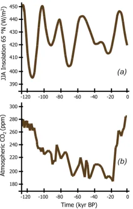
under study (Fig. 1); the lowest value of summer insolation (JJA) at 65◦_{N occurs at}

113 kyr BP (395 W/m2) and the highest ones are reached at 125 kyr BP and 101 kyr

BP (>450 W/m2).

A critical problem to simulate a full glacial-interglacial cycle, and especially the in-ception of the ice sheets, is to obtain realistic precipitation patterns. In our model,

15

the precipitation from a given CLIMBER grid box uniformly falls on the

correspond-ing GREMLINS grid points. Therefore, due to the difference of resolution between

CLIMBER and GREMLINS, the simulated precipitation patterns often suffer from

short-comings, in particular over high altitude regions where most precipitations actually fall on the wind exposed slope of the first mountain range encountered by the air parcels.

20

The comparison between the simulated present-day precipitations (PRCCLIMBER) with

those provided by the CRU climatology (PRCCRU) shows that the climate model tends

to significantly underestimate the precipitation over the areas extending from the east-ern part of the Scandinavian Alps to the Barents-Kara sea region. Conversely, over Beringia precipitations are overestimated. To account for these discrepancies, we

ap-25

ply to the simulated CLIMBER precipitation a corrective factor PRC_CRU/PRC_CLIMBER

(13)

CPD

5, 1013–1053, 2009

ice sheets

S. Bonelli et al.

Title Page

Tables Figures

◭ ◮

Back Close

Full Screen / Esc

3.2 Results

The objective of the baseline experiment is to examine whether the coupled model is able to simulate a realistic evolution of major NH ice sheets during the last glacial-interglacial cycle. In particular, we are interested in capturing the main features of glacial inceptions, expansions or retreats shown by the available records in terms of

5

timing, geography and amplitude of sea-level variations. Our approach focuses on the large-scale processes and on the phase relationships between the external forcings and the periods of growth and retreat of major ice sheets. Due to the absence of rep-resentation of rapid ice flow dynamics in the ISM, the issue of rapid climate variability is not addressed in the present work.

10

3.2.1 Simulated ice sheet topography

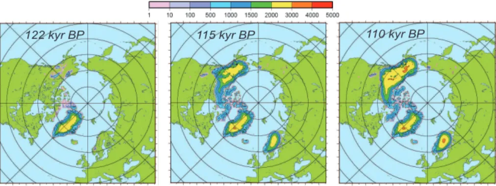
Figure 2 shows the spatial distribution of the simulated ice sheets during the first phase of glacial inception, respectively at 122, 115 and 110 kyr BP.

At 122 kyr BP (Fig. 2) the model produces small ice caps in northwestern Canada, in the northern Rocky Mountains and over both the Ellesmere Island and the eastern

15

part of the Baffin Island in the Canadian Archipelago. These areas represent the first

simulated nucleation zones, which rapidly evolve into a much larger ice sheet at 115 kyr BP.

At 115 kyr BP the simulated summer temperature is negative over most of Green-land, the Canadian Archipelago and the Rocky Mountains close to the Canada-Alaska

20

border (Fig. 3), where we simulate a positive mass balance of more than 0.5 m/y (not

shown). Continental ice spreads over most of Alaska’s mainland, the northern Rocky Mountains and reaches the northwestern borders of Hudson-Bay. Its simulated thick-ness exceeds 2000 m in its central parts. We also simulate areas of negative summer

temperature over Fennoscandia. A relatively large ice sheet appears between 60◦_N

25

and 70◦_{N in the Scandinavian Alps. In some places its thickness is higher than 2000 m;}

(14)

CPD

5, 1013–1053, 2009

ice sheets

S. Bonelli et al.

Title Page

Tables Figures

◭ ◮

Back Close

Full Screen / Esc

The total NH ice volume further increases at 110 kyr BP despite the fact that summer insolation is larger than at 115 kyr BP. At this period, the North American ice sheet now thickens to more than 3000 m in central Alaska, and occupies a large portion of the 60–

70◦_{N latitudinal belt west of Hudson Bay (Fig. 2). Most of the Canadian Archipelago is}

ice-covered, but the isolated island ice sheets do not coalesce into a larger ice complex,

5

which is likely due to a crude representation of the ice advance over marine areas. At this time, the model also produces a thicker ice sheet over Eurasia, but its extent is significantly smaller than that of the North American ice sheet. Continental ice is

mainly located over the Scandinavian Peninsula and does not spread south of 60◦_N.

The timing of glacial onset is consistent with the reconstructed first phase of

glacia-10

tion, as inferred from sea-level data (Yokoyama et al., 2001; Camoin et al., 2001; Lam-beck and Chappell, 2001; Waelbroeck et al., 2002; Siddall et al., 2003; Bintanja et al., 2005), geomorphological observations (Boulton and Clark, 1990; Svendsen et al., 2004) and previous modelling studies (Tarasov and Peltier, 1997; Berger et al., 1998; Kageyama et al., 2004; Calov et al., 2005; Kubatzki et al., 2006). Nevertheless,

obser-15

vational data (Andrews and Barry, 1978) indicate that the regions of ice-sheet inception

in North America were those bordering the eastern coast, and in particular Baffin

Is-land, the Quebec-Labrador sector and the northeastern Keewatin region. The model

correctly captures the glacial onset on Baffin and Ellesmere Islands, but does not

pro-duce ice accumulation over Quebec. Conversely, it tends to overestimate ice growth

20

on northwestern Rocky Mountains. Paleoenvironmental records indicate that, at the early phase of glacial onset, this region was likely as warm as today, or even warmer, and substantially ice-free (Clark et al., 1993). Indeed, the Cordilleran ice sheet does

not seem to have appeared before the late isotopic stage 4 or 5 (i.e. ∼75 kyr BP),

when the Laurentide ice sheet (LIS) was high enough to displace the jet stream

caus-25

ing precipitations to fall over the Rocky Mountains (Roe and Lindzen, 2001). This is in disagreement with our results, because the coupled model simulates low summer

temperatures in some regions of the Rocky Mountains at 123 kyr BP (down to−5◦C

(15)

precipi-CPD

5, 1013–1053, 2009

ice sheets

S. Bonelli et al.

Title Page

Tables Figures

◭ ◮

Back Close

Full Screen / Esc

tations are overestimated in the interior of the Rockies because, in the model, they do not represent a strong barrier to prevent precipitation from falling over this region. As

a result, the simulated mean annual precipitation is greater than 1000 mm/yr at 122 kyr

BP. This is also valid for present-day conditions, since the model overestimates

precip-itation by∼150% compared to the CRU climatology in central areas of the Rockies.

5

Glacial inception in the northwestern Rocky Mountains is not unusual in model studies and has been found by Kageyama et al. (2004) with a previous version of this model, and by Charbit et al. (2007) in GCM-driven simulations. The model also produces a glacial onset over Alaska, in disagreement with observations (Boulton and Clark, 1990). This is a common problem for coupled climate-ISM simulations (Deblonde and

10

Peltier, 1991; Peltier and Marshall, 1995). Previous studies conducted with GCMs sug-gest that a more realistic modelling of vegetation over Beringia has a strong impact on local albedo and atmospheric circulation patterns (Wyputta et al., 2001). Refined vegetation indirectly leads to circulation changes that generate a warm anomaly over Alaska and Eastern Siberia, which, in turn, reduces the accumulation of grounded ice.

15

Furthermore, previous works argue that the lack of a simulated Kuroshio Current may be also responsible of colder climatic conditions in these regions, thus fostering snow accumulation (Peltier and Marshall, 1995). Simulated ice inception and growth over Alaska and Beringia results from the combination of both coarse climate model res-olution and from these regional and important features of the climate system, poorly

20

represented in our coupled model.

At 110 kyr BP, geomorphologial reconstructions suggest the presence of an ice dome in the Quebec-Labrador region, and a coalesced ice sheet over the Canadian Archipelago (Boulton and Clark, 1990). The coupled CLIMBER-GREMLINS model does not produce any Quebec-Labrador dome due to warm North Atlantic (and Hudson

25

Bay) SSTs simulated by the CLIMBER model, affecting the climate of nearby regions:

at 50◦_{N the simulated mean summer SSTs range between 10 and 12}◦_{C in}

northwest-ern Atlantic, whereas they range between 8 and 12◦_{C on Quebec’s mainland at the}

(16)

CPD

5, 1013–1053, 2009

ice sheets

S. Bonelli et al.

Title Page

Tables Figures

◭ ◮

Back Close

Full Screen / Esc

the production of a single massive ice sheet over the Canadian Archipelago and the advance of ice over Hudson Bay. In the same way, the model does not simulate ice over the Barents-Kara sea region, as suggested by Svendsen et al. (2004), whereas continental ice over Scandinavia is properly reproduced. Observational data show that the 110 kyr BP period coincides with the maximum ice extent after the first glacial

in-5

ception and is characterized by a major contribution from the LIS. A smaller ice sheet exists in the mountainous region of the Scandinavian Peninsula, but its contribution to NH ice volume is minor (Kleman et al., 1997). This feature clearly appears in our model results.

The spatial distribution of the simulated ice sheets from 110 kyr BP to present-day is

10

plotted on Fig. 4 for six di_fferent key periods: 100, 75, 60, 30, 21 and 0 kyr BP. These

snapshots refer to different stadial or interstadial states and correspond to pronounced

phases of glacial expansion or retreat.

Between 110 and 100 kyr BP (Figs. 2 and 4), the ice sheet covering Alaska and the northwestern part of Canada increases, mainly due to the elevation of the ice thickness.

15

Conversely, the southern part of Baffin Island is ice-free and no ice is simulated in this

region at latitudes lower than 70◦_{N. At this time, observational data suggest that the}

LIS was partly melted (Andrews et al., 1983). The model does not produce any large ice cap in the Fennoscandian region. Only a small mountain ice sheet survives in high altitude regions of the Scandinavian Alps, but its extent is considerably smaller than

20

the one simulated at 110 kyr BP, in agreement with the reconstructions from Mangerud et al. (2004). The simulation correctly produces the melting of the Fennoscandian ice

sheet (FIS), as well as that of the southern part of Ba_ffin Island. Nevertheless, ice

thickness increases over northwestern Canada and Alaska due to the snow/ice albedo

and elevation effects. The North American ice sheet is huge enough to sustain itself

25

under increasing insolation (Fig. 2).

At 75 kyr BP, the simulated ice sheet covers Alaska’s mainland and spreads further

south, down to 50◦_{N (Fig. 4); a massive ice sheet is produced over the Canadian}

(17)

CPD

5, 1013–1053, 2009

ice sheets

S. Bonelli et al.

Title Page

Tables Figures

◭ ◮

Back Close

Full Screen / Esc

most of the islands of the Canadian Archipelago, including the southern part of Baffin

Island. As suggested by observations (Kleman et al., 1997), no ice sheet builds up in non-mountainous areas of the Fennoscandian Peninsula. Indeed, consistently with reconstructions, the extent of the simulated FIS at 75 kyr BP (MIS5a) is smaller than the one corresponding to the 110 kyr BP period (MIS5d) and comparable to the 100 kyr

5

BP snapshot (Kleman et al., 1997; Svendsen et al., 2004).

At 60 kyr BP, the model produces a large ice sheet west of Hudson Bay (Fig. 4).

This complex develops as far as∼50◦N, spreading over most of the North American

continent. The ice volume covering the Canadian Archipelago and Alaska has also slightly increased. Continental ice builds up in the Quebec-Labrador region, reaching

10

a thickness of more than 2000 m in central areas and forming the second largest ice sheet in North America mainland. The model simulates the presence of a Keewatin ice dome in agreement with observational data (Boulton and Clark, 1990), but under-estimates the Laurentide ice complex: the Labrador dome is smaller than that inferred from reconstructions and there is no ice over Hudson Bay.

15

The simulation of an ice sheet over the Scandinavian region is consistent with geo-morphological reconstructions (Svendsen et al., 2004). However, in contradiction with geological data, the Barents-Kara sea region remains ice-free (Mangerud et al., 2002; Svendsen et al., 2004). As previously mentioned, this discrepancy is likely related to the fact that the ice shelves are only crudely represented in the ISM.

20

Geomorphological data show that the 60 kyr BP period is characterized by the pres-ence of large, persistent ice sheets over both North America and Eurasia (Boulton and Clark, 1990; Mangerud et al., 2002; Svendsen et al., 2004). With the exception of the above-mentioned regional discrepancies, the model reasonably produces this major

feature. Indeed, the MIS5/MIS4 transition (∼75 kyr BP) outlines a pronounced switch

25

(18)

CPD

5, 1013–1053, 2009

ice sheets

S. Bonelli et al.

Title Page

Tables Figures

◭ ◮

Back Close

Full Screen / Esc

the post-LGM period. Thus, the MIS5/MIS4 transition may be considered as the be-ginning of the true glacial phase. Glacial conditions are now widely spread and larger ice-induced feedbacks contribute to a further cooling of the system. Between 60 kyr and 30 kyr BP, the Eurasian ice volume does not significantly change, whereas the ice volume over the Quebec-Labrador sector and the Keewatin region has increased.

5

After 30 kyr BP, the simulated ice volume increases again until ∼21 kyr BP (LGM)

(Fig. 4). The system switches towards more pronounced glacial conditions, similarly to the cold shift observed during the MIS5/MIS4 transition. At the LGM, the Labrador

and Quebec regions are ice-covered and the LIS stretches south of 50◦_{N. Consistently}

with reconstructions, the simulated ice masses completely cover the St. Lawrence

10

Gulf, as well as the Canadian regions bordering the Atlantic Ocean (Dyke et al., 2002). However, geological reconstructions indicate the existence of two domes centered over the Keewatin region and the Quebec-Labrador plateau. The absence of a bi-domed ice sheet may be due to the ISM, which does not account for sediment deformation and for the ice fast flow resulting from water-saturated sediments. According to Tarasov

15

and Peltier (2004), this is a prerequisite to properly simulate a multi-domed ice surface topography. Another discrepancy with observations (Dyke et al., 2002) lies in the fact that a huge ice sheet is simulated over Beringia.

At the LGM, the FIS spreads over the whole Baltic region and the British Islands, reaching a thickness of more than 3000 m in its central dome. The model also simulates

20

the junction between the British Isles and the southern part of Scandinavia. However, it still underestimates the ice cover in the Barents-Kara sea region (Svendsen et al., 2004). Interestingly, a small mountain ice cap develops in the Alps, but its volume is negligible compared to major ice sheets. Iceland and the Faroe Islands are also completely ice covered.

25

(19)

CPD

5, 1013–1053, 2009

ice sheets

S. Bonelli et al.

Title Page

Tables Figures

◭ ◮

Back Close

Full Screen / Esc

features of LGM ice topography and simulates large ice sheets over both Eurasia and North America, in agreement with geomorphological investigations (Boulton and Clark, 1990; Mangerud et al., 2002; Dyke et al., 2002; Svendsen et al., 2004).

At 0 kyr (Fig. 4), the model produces the complete retreat of continental ice over most of the North American continent, as well as over Eurasia. The only exceptions are small

5

residual ice sheets in northern Alaska and in mountainous areas of the Scandinavian Peninsula.

3.2.2 Ice-equivalent sea level change

The atmospheric CO2 concentration and the summer insolation, as well as the

corre-sponding simulated ice-equivalent sea level change due to major NH ice sheets, are

10

plotted in Fig. 5. The computed ice-equivalent sea level is also directly compared to the relative sea-level curve from Waelbroeck et al. (2002) inferred from benthic iso-topic records (Fig. 5b). It is important to note that the simulated sea level only refers to the contribution of ice changes in the NH and does not account for the Antarctic contribution (Philippon et al. 2006), whereas the curve from Waelbroeck et al. (2002)

15

represents a global signal.

Sea-level change is directly dependent on ice sheet evolution. The ice-equivalent sea level inferred from our model simulation is computed as follows:

SL₌−Vol

S ×

_δ

I

δSW

+GSL

where SL represents the ice-equivalent sea level (m s.l.e.), Vol the NH total ice volume

20

(m3), S the global sea surface (3.64×1014 m2), δI the ice density at 0◦C (917 g/cm3),

δSW the averaged sea water density at 0◦C and 35 p.s.u. (1028 g/cm

3

) and GSL is the contribution of the initial Greenland ice sheet to sea-level change (7.3 m).

We assume that the oceanic area is constant and equal to the present-day one since it does not significantly change throughout the last glacial-interglacial cycle.

(20)

CPD

5, 1013–1053, 2009

ice sheets

S. Bonelli et al.

Title Page

Tables Figures

◭ ◮

Back Close

Full Screen / Esc

A first drop of sea level is observed between 122 kyr and 110 kyr BP and is correlated

with a sharp decrease of summer insolation at 65◦_{N. This timing is consistent with the}

sea level reconstruction from benthic records (Waelbroeck et al., 2002). At 110 kyr BP, the simulated seal level has decreased by 28.5 m, that is about 15 m higher than the one obtained by Waelbroeck et al. (2002). This is consistent with the fact that no ice

5

is simulated over the Labrador-Quebec sector and the Barents-Kara region (Fig. 4), in contradiction with the observations (discussion in Sect. 3.2.1). The presence of an ice sheet covering a large part of Alaska (Fig. 4) increases the simulated sea level drop, but does not compensate the lack of ice over these regions. However, as previ-ously mentioned, the sea level reconstruction (Fig. 5b) corresponds to a global signal

10

(Waelbroeck et al., 2002), whereas the sea level simulated in our experiment only ac-counts for the contribution of NH ice sheets. A potential contribution from the Antarctic ice sheet is thus not considered. Indeed, Duplessy et al. (2007, 2008) suggest that the West Antarctic ice sheet was partly destabilized during the last interglacial period and that its further expansion likely contributed to the sea level drop recorded after the

15

Eemian.

Between 110 and 100 kyr BP, the ice-equivalent sea level evolution simulated by the coupled model slightly increases by 6.5 m (Fig. 5c). This corresponds to the disap-pearance of the FIS (Fig. 4). During this period a rapid increase of summer insolation

at 65◦_{N is observed and reaches one of the maxima of the last 126-kyr (Figs. 1 and}

20

5a), whereas the atmospheric CO2 undergoes a first significant decrease from 250 to

225 ppm. A new sea level drop is observed at 90 kyr BP (−38.5 m), then followed by

a slight increase until∼75 kyr BP.

During this first period of the glacial cycle (126–75 kyr BP), the evolution of the sim-ulated ice sheets appears therefore to be correlated with the summer insolation signal,

25

suggesting that this is the major factor triggering glacial expansion or retreat of the ice sheets.

(21)

CPD

5, 1013–1053, 2009

ice sheets

S. Bonelli et al.

Title Page

Tables Figures

◭ ◮

Back Close

Full Screen / Esc

a significant decrease of summer insolation at 65◦_{N, combined to low atmospheric}

CO2concentrations (190 ppm at 65 ka BP). The decrease of both forcing factors makes

the system switch towards colder conditions, characterized by a rapid sea-level drop

(∼−24 m in less than 15 kyr in our simulations) and by the existence of long-lasting ice

sheets over both Eurasia and North America (Fig. 4), which corresponds to the

ac-5

tual beginning of the full NH glaciation (e.g. Jouzel et al., 2007). The newly re-formed

FIS persists even under increasing summer insolation after∼70 kyr BP (Fig. 4), which

proves that the atmospheric CO2 concentration is low enough to counterbalance the

insolation radiative effect. As shown for the first phase of glacial inception, the FIS may

build up in presence of low summer insolation and relatively high atmospheric CO₂,

10

but the associated positive feedbacks due to increased albedo and surface elevation

are not efficient enough to prevent it from melting under unfavorable orbital

param-eters (i.e. increasing insolation). This sequence of glaciation events shows that the

decrease of summer insolation alone is sufficient to explain the expansion of grounded

ice over North America and Eurasia. Nevertheless, the FIS needs low atmospheric

15

CO₂concentration to survive to subsequent increases of insolation. This explains why

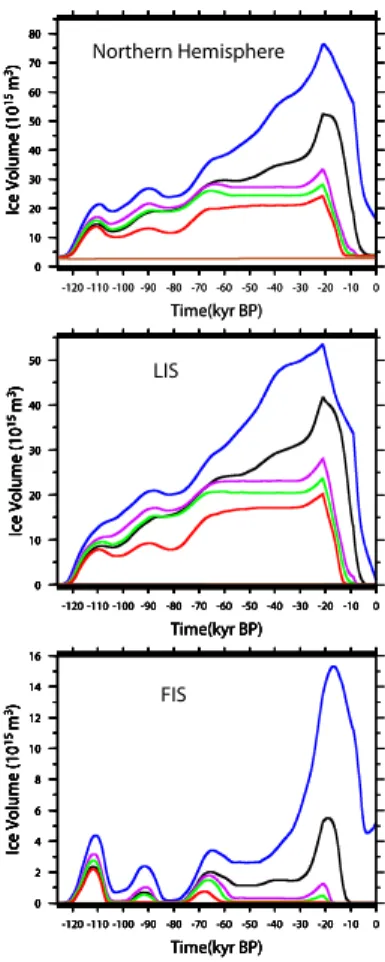
the simulated FIS can sustain itself only after∼75 kyr BP and until the LGM (Fig. 6).

The sea level drop between 60 and 30 kyr BP is less pronounced than that occur-ring between 75 and 65 kyr BP. Duoccur-ring this period the simulated sea level evolution is smoother than the one inferred from benthic foraminifera records (Waelbroeck et al.,

20

2002) and no abrupt expansion or regression of the ice volume is reproduced. The sim-ulated ice sheets are large enough to counterbalance, via the ice albedo and elevation

effects, the relatively high values of insolation prevailing during the 50–30 kyr BP period.

Moreover, the maintenance of the ice sheets is also supported by rather low CO2

lev-els (200 to 220 ppm). The data-based relative sea level curve shows a slight decrease

25

after 50 kyr BP (Waelbroeck et al., 2002). The coupled model is not sensitive enough

to decreasing insolation when summer values remain higher than 420 W/m2 and the

(22)

rep-CPD

5, 1013–1053, 2009

ice sheets

S. Bonelli et al.

Title Page

Tables Figures

◭ ◮

Back Close

Full Screen / Esc

resentation of the ice shelves and of basal hydrology processes in the ISM could help produce results better fitting to data.

Around 30 kyr BP we observe a further pronounced expansion of main NH ice sheets

in response to a new decrease of both insolation and atmospheric CO₂concentration.

This expansion is associated to a sea level decrease of∼39 m in less than 10 kyr. At

5

the LGM, the simulated ice equivalent sea level lowering is−121.5 m (Fig. 5c). The

timing of the maximum sea level drop is consistent with reconstructions (Waelbroeck et al., 2002; Siddall et al., 2003). The simulated LGM ice volumes of the LIS and the

FIS amount to 41.8×1015m3 and 5.3×1015m3, respectively (Table 2). These results

are in agreement with the findings from Lambeck et al. (2000); on the contrary, the

10

simulated LIS is larger than the one described in the ICE-5G reconstruction (Peltier, 2004), whereas the simulated FIS volume is lower.

At the LGM, the Antarctic contribution to sea-level change computed by Philippon et al. (2006) with the same climate model coupled to a 3-D Antarctic ISM (Ritz et al., 2001) ranges between 9.5 and 17 m. Therefore, we can estimate the simulated

15

ice-equivalent sea-level at the LGM to range between−131 m and−138.5 m. These

values lie within the upper bound of the most commonly accepted reconstructions,

ranging between ∼−110 and −143 m at the LGM (Yokoyama et al., 2001; Lambeck

and Chappell, 2001; Camoin et al., 2001; Waelbroeck et al., 2002; Siddall et al., 2003; Bintanja et al., 2005). Compared to previous modeling works (Tarasov and Peltier,

20

1997; Zweck and Huybrechts, 2005), the simulated LGM sea level is∼10 m lower due

(23)

CPD

5, 1013–1053, 2009

ice sheets

S. Bonelli et al.

Title Page

Tables Figures

◭ ◮

Back Close

Full Screen / Esc

4 Sensitivity tests

4.1 Experimental set-up

To better investigate the effect of both atmospheric CO2 concentration and insolation

on major NH ice sheets, we perform a set of sensitivity tests. These experiments are conducted as previously described for the baseline (BSL) experiment, but under

con-5

stant insolation or constant atmospheric CO2 concentration (Table 1). The INSO-126

experiment is run under constant 126-kyr BP insolation and pCO2 evolution inferred

from the Vostok ice core (Petit et al., 1999). In this test, summer insolation at 65◦_{N is}

equal to 452 W/m2and is therefore particularly unfavorable for glacial onset. The

sen-sitivity tests CO2-280, CO2-250, CO2-235 and CO2-200 are performed by driving the

10

coupled CLIMBER-GREMLINS model with BSL-insolation (Berger, 1978) and constant

CO2 concentration fixed to 280, 250, 235 and 200 ppm, respectively. These tests are

designed to investigate a potential CO2threshold effect on the evolution of major NH

ice sheets and their different sensitivity to external forcings.

4.2 Results

15

The temporal evolution of the simulated ice volumes is plotted on Fig. 6 for all the transient sensitivity experiments performed in this study. These results are compared with those obtained in the baseline (BSL) experiment.

In the CO₂-280 test (Fig. 6), the simulated LIS ice volume during the early phase

of the glacial inception (126–110 kyr BP) does not significantly differ from the one

pro-20

duced in the BSL experiment (Fig. 6). This confirms that the early glacial build-up is primarily driven by decreasing summer insolation (Figs. 1 and 5a) since the model still

produces ice development over North America and Eurasia for a CO2level of 280 ppm,

typical of interglacial periods. Conversely, after 110 kyr BP the CO2-280 ice volume

re-mains significantly lower than the BSL one. A similar result is obtained in the CO₂-250

25

(24)

CPD

5, 1013–1053, 2009

ice sheets

S. Bonelli et al.

Title Page

Tables Figures

◭ ◮

Back Close

Full Screen / Esc

than in the baseline experiment (28.2×1015m3vs. 52.5×1015m3for the NH ice sheets

at the LGM, Table 2).

When the atmospheric CO₂further decreases to 235 ppm (CO₂-235), half-way

be-tween typical glacial and interglacial values (Petit et al., 1999), the LIS build-up is faster and slightly larger than in BSL until 65 kyr BP, but remains lower than in BSL during the

5

65–21 kyr BP interval. For this latter period the 65◦_{N summer insolation is higher than}

420 W/m2 until ∼30 kyr BP. This value is too high to trigger any significant ice

accu-mulation when the atmospheric CO2concentration is fixed to 235 ppm (or higher), and

the growth of the ice sheets stops and stabilizes between 65 and 30 kyr BP in tests

CO2-280, CO2-250 and CO2-235 (Fig. 6). Throughout this period, the atmospheric

10

CO2concentration in BSL actually varies between 190 and 220 ppm, thus contributing

to a further cooling of the climate system. This cooling adds up to the positive feedback

effects due to existing ice sheets and results in a larger LGM ice volume in BSL. On

the contrary, for constant CO2 concentrations higher than 235 ppm these feedbacks

only prevent the LIS from melting, but they are not sufficient to trigger a further glacial

15

expansion until the pronounced decrease of summer insolation observed after 30 kyr BP.

In the CO₂-200 experiment, the CO₂concentration is low enough to produce a large

glacial inception over North America and Eurasia as soon as the early phase of glacia-tion. At 110 kyr BP, the North American and Fennoscandian ice volumes are 149% and

20

200% larger than those simulated in BSL. At the LGM the simulated LIS and FIS ice

volumes are, respectively 53.5×1015m3and 13.6×1015m3, compared to 41.8×1015m3

and 5.3×1015m3in the BSL experiment.

Although the behavior of both ice sheets appears to be quite similar, the excess of

ice simulated over Fennoscandia under a 200 ppm CO2 level, compared to the BSL

25

test, is considerably larger than the ice excess obtained over North America (257% for

FIS, 128% for LIS). Moreover, a stable, long-lasting FIS is only formed after∼75 kyr BP

in BSL and in the CO2-200 experiments.

(25)

CPD

5, 1013–1053, 2009

ice sheets

S. Bonelli et al.

Title Page

Tables Figures

◭ ◮

Back Close

Full Screen / Esc

atmospheric CO₂decreases from 235 ppm to 200 ppm, the effect of orbital

configura-tions favorable for glacial expansion (Berger, 1978) is amplified. The lower CO2values

also provide a further cooling, necessary to prevent the FIS from melting during the 65– 30 kyr BP interval and resulting in the build-up of a large European ice complex at the

LGM. Conversely, higher CO2concentrations prevent from significant ice growth over

5

Fennoscandia at the LGM in experiments CO2-235, CO2-250 and CO2-280. Therefore,

the Fennoscandian ice sheet appears to be more sensitive to atmospheric CO₂

con-centration than the North American ice sheet. This confirms our conclusions obtained from the analysis of the relationship between external forcings and the evolution of ice volume in the baseline experiment (Sect. 3).

10

5 Summary and conclusions

In this work we study the evolution of major NH ice sheets during the last glacial-interglacial cycle. The mechanisms leading to the onset, growth and decay of the ice sheets have been explored with a climate model of intermediate complexity, coupled to a 3-D thermo-mechanical ISM.

15

The CLIMBER-GREMLINS model reproduces the main phases of advance and re-treat of Northern Hemisphere ice sheets during the last glacial cycle, although the amplitude of these variations is less pronounced than those based on global sea level

reconstructions. At the LGM, the simulated ice volume is 52.5×1015m3and the spatial

distribution of both the American and Eurasian ice complexes is in reasonable

agree-20

ment with observations, with the exception of the marine parts of these ice sheets.

We investigate the responses of the two major NH ice sheets to atmospheric CO2

concentration and insolation, as well as their sensitivity to these forcings. Our

simu-lations suggest that the Laurentide ice sheet has a different dynamics of development

compared to the Fennoscandian ice sheet, since they do not respond with the same

25

sensitivity to atmospheric CO₂ concentration. We simulate the early build-up of

(26)

CPD

5, 1013–1053, 2009

ice sheets

S. Bonelli et al.

Title Page

Tables Figures

◭ ◮

Back Close

Full Screen / Esc

BP. The evolution of this ice complex is largely driven by the insolation forcing through-out the whole 126-kyr cycle. Conversely, the model produces glacial inception on the Fennoscandian Peninsula in the early phases of glaciation, but this early ice sheet is not stable enough to survive to following periods of increasing summer insolation.

Indeed, both weak summer insolation and low atmospheric CO₂ concentration are

5

necessary to trigger a long-lasting glaciation over Eurasia. Consistently with recon-structions (Svendsen et al., 2004), a long-lasting FIS only appears after 75 kyr BP in correspondence of the MIS5/MIS4 cold transition.

As proposed by Milankovitch (Milankovitch, 1941), changes in summer insolation

trigger the ice sheets inception. Nevertheless, variations in atmospheric CO2

concen-10

tration, as well as climate-ice sheet feedbacks, are important mechanisms a_ffecting

the duration and intensity of cold/warm periods and the extent and altitude of major NH ice sheets. Sensitivity tests conducted under standard insolation and for various

constant CO₂levels demonstrate that the FIS is more sensitive to the atmospheric CO₂

concentration than the LIS. In our simulations, the build-up of a stable FIS responds to

15

a threshold behaviour to CO2concentration and its development is drastically different

when the atmospheric CO₂decreases from 235 to 200 ppm.

This work also underlines the limits of the coupled model. These are either due to the CLIMBER coarse spatial resolution, unable to capture some important regional features of the climate system (i.e. influence of the Rockies on the precipitation over

20

the American continent and the existence of the Kuroshio Current in North Pacific), or to identified missing processes in the ISM, such as the absence of rapid ice flow dynamics and sediment deformation. The addition of these mechanisms in the ISM should improve the spatial distribution of simulated ice over marine regions such as Hudson Bay or the Barents-Kara sea sector.

25

Acknowledgement. This work was carried out in the framework of the French ANR PICC

(27)

CPD

5, 1013–1053, 2009

ice sheets

S. Bonelli et al.

Title Page

Tables Figures

◭ ◮

Back Close

Full Screen / Esc

to A. Ganopolski and C. Ritz for fruitful discussion, and to Lev Tarasov and for his constructive comments which helped us improve the writing of the manuscript.

The publication of this article is financed by CNRS-INSU.

5

References

Abe-Ouchi, A., Segawa, T., and Saito, F.: Climatic Conditions for modelling the Northern Hemi-sphere ice sheets throughout the ice age cycle, Clim. Past, 3, 423–438, 2007,

http://www.clim-past.net/3/423/2007/.

Adkins, J. F. B., Boyle, E. A., Keigwin, L., and Cortijo, E.: Variability of the North Atlantic

ther-10

mohaline circulation during the last interglacial period, Nature, 390(6656), 154–156, 1997. Andrews, J. T. and Barry, R. G.: Glacial inception and disintegration during last glaciation, Ann.

Rev. Earth Planet. Sci., 6, 205–228, 1978.

Andrews, J. T., Shilts, W. W., and Miller, G. H.: Multiple deglaciations of the Hudson-Bay low-lands, Canada, since deposition of the Missinaibi (Last-Interglacial Questionable Formation),

15

Quaternary Res., 19(1), 18–37, 1983.

Berger, A. L.: Long-term variations of daily insolation and quaternary climatic changes, J. At-mos. Sci., 35(12), 2362–2367, 1978.

Berger, A., Loutre, M. F., and Gallee, H.: Sensitivity of the LLN climate model to the

astronomi-cal and CO₂forcings over the last 200 ky. Clim. Dynam., 14(9), 615–629, 1998.

20

Berger, A., Li, X. S., and Loutre, M. F.: Modelling Northern Hemisphere ice volume over the last 3 Ma, Quaternary Sci. Rev., 18(1), 1–11, 1999.

Bintanja, R., van de Wal, R. S. W., and Oerlemans, J.: Modelled atmospheric temperatures and global sea levels over the past million years, Nature, 437(7055), 125–128, 2005. Boulton, G. S. and Clark, C. D.: The Laurentide ice-sheet through the last glacial cycle – The

(28)

CPD

5, 1013–1053, 2009

ice sheets

S. Bonelli et al.

Title Page

Tables Figures

◭ ◮

Back Close

Full Screen / Esc

topology of drift lineations as a key to the dynamic behavior of former ice sheets, Trans. Roy. Soc. Edinburgh – Earth Sci., 81, 327–347, 1990.

Braithwaite, R. J.: Positive degree-day factors for ablation on the Greenland ice-sheet studied by energy-balance modeling, J. Glaciol., 41(137), 153–160, 1995.

Brovkin, V., Ganopolski, A., and Svirezhev, Y.: A continuous climate-vegetation classification

5

for use in climate-biosphere studies, Ecol. Model., 101(2–3), 251–261, 1997.

Brovkin, V., Bendtsen, J., Claussen, M., et al.: Carbon cycle, vegetation, and climate dynamics in the Holocene: Experiments with the CLIMBER-2 model, Global Biogeochem. Cy., 16(4), 1139, doi:10.1029/2001GB001662, 2002.

Calov, R., Ganopolski, A., Clausse, M., et al.: Transient simulation of the last glacial inception.

10

Part I: glacial inception as a bifurcation in the climate system, Clim. Dynam., 24(6), 545–561, 2005.

Calov, R., Ganopolski, A., Clausse, M., et al.: Transient simulation of the last glacial inception. Part II: sensitivity and feedback analysis, Clim. Dynam., 24(6), 563–576, 2005.

Camoin, G. F., Ebren, P., Eisenhauer, A., et al.: A 300 000-yr coral reef record of sea level

15

changes, Mururoa atoll (Tuamotu archipelago, French Polynesia), Palaeogeo. Palaeoclima-tol, Palaeoecol., 175(1–4), 325–341, 2001.

Chapman, M. R., Shackleton, N. J., and Duplessy, J. C.: Sea surface temperature variability during the last glacial-interglacial cycle: assessing the magnitude and pattern of climate change in the North Atlantic, Palaeogeo. Palaeoclimatol. Palaeoecol., 157(1–2), 1–25, 2000.

20

Charbit, S., Kageyama, M., Roche, D., et al.: Investigating the mechanisms leading to the deglaciation of past continental Northern Hemisphere ice sheets with the CLIMBER-GREMLINS coupled model, Global Planet. Change, 48(4), 253–273, 2005.

Charbit, S., Ritz, C., Philippon, G., Peyaud, V., and Kageyama, M.: Numerical reconstructions of the Northern Hemisphere ice sheets through the last glacial-interglacial cycle, Clim. Past,

25

3, 15–37, 2007,

http://www.clim-past.net/3/15/2007/.

Clark, P. U., Clague, J. J., Curry, B. B., et al.: Initiation and development of the Laurentide and Cordilleran ice sheets following the last interglaciation, Quaternary Sci. Rev., 12(2), 79–114, 1993.

30

Clark, P. and Pollard, D.: Northern Hemisphere ice-sheet influences on global climate change, Science, 286(5442), 1104–1111, 1999.