Grounding line transient response in marine ice sheet models

(1)

TCD

6, 3903–3935, 2012

Grounding line transient response

A. S. Drouet et al.

Title Page

Abstract Introduction

Conclusions References

Tables Figures

◭ ◮

Back Close

Full Screen / Esc

Printer-friendly Version Interactive Discussion

Discussion

P

a

per

|

Dis

cussion

P

a

per

|

Discussion

P

a

per

|

Discussio

n

P

a

per

|

The Cryosphere Discuss., 6, 3903–3935, 2012 www.the-cryosphere-discuss.net/6/3903/2012/ doi:10.5194/tcd-6-3903-2012

The Cryosphere Discussions

This discussion paper is/has been under review for the journal The Cryosphere (TC). Please refer to the corresponding final paper in TC if available.

Grounding line transient response in

marine ice sheet models

A. S. Drouet1, D. Docquier2, G. Durand1, R. Hindmarsh3, F. Pattyn2, O. Gagliardini1,4, and T. Zwinger5

1

UJF – Grenoble 1/CNRS, Laboratoire de Glaciologie et G ´eophysique de l’Environnement (LGGE) UMR 5183, Grenoble, 38041, France

2

Laboratoire de Glaciologie, Universit ´e Libre de Bruxelles, CP160/03, Av F.Roosevelt 50, 1050 Brussels, Belgium

3

British Antarctic Survey, Natural Environment Research Council, Madingley Road, Cambridge CB3 0ET, UK

4

Institut Universitaire de France, Paris, France 5

CSC-IT Center for Science Ltd., Espoo, Finland

Received: 24 July 2012 – Accepted: 23 August 2012 – Published: 18 September 2012

Correspondence to: G. Durand (durand@lgge.obs.ujf-grenoble.fr)

Published by Copernicus Publications on behalf of the European Geosciences Union.

(2)

TCD

6, 3903–3935, 2012

A. S. Drouet et al.

Title Page

Tables Figures

◭ ◮

Back Close

Full Screen / Esc

Discussion

P

a

per

|

Dis

cussion

P

a

per

|

Discussion

P

a

per

|

Discussio

n

P

a

per

|

Abstract

Marine ice sheet stability is mostly controlled by the dynamics of the grounding line, i.e., the junction between the grounded ice sheet and the floating ice shelf. Grounding line migration has been investigated in the framework of MISMIP (Marine Ice Sheet Model Intercomparison Project), which mainly aimed at investigating steady state

solu-5

tions. Here we focus on transient behaviour, executing short-term simulations (200 yr) of a steady ice sheet perturbed by the release of the buttressing restraint exerted by the ice shelf on the grounded ice upstream. The transient grounding line behaviour of four different flowline ice sheet models has been compared. The models differ in the physics implemented (full-Stokes and Shallow Shelf Approximation), the numerical approach,

10

as well as the grounding line treatment. Their overall response to the loss of buttressing is found to be consistent in terms of grounding line position, rate of surface elevation change and surface velocity. However, large discrepancies (>100 %) are observed in terms of ice sheet contribution to sea level. Despite the recent important improvements of marine ice sheet models in their ability to compute steady-state configurations, our

15

results question models’ capacity to compute reliable sea-level rise projections.

1 Introduction

A range of observational methodologies have shown that significant loss of Antarctic ice mass has occurred over the past decade (Wingham et al., 2006; Rignot et al., 2008, 2011; Velicogna, 2009; Pritchard et al., 2012). Increased basal melt of ice shelves

20

appears to be the primary control on Antarctic ice sheet loss, owing to the way the resultant thinning in ice-shelves reduces buttressing of grounded ice by the shelves, which leads to an acceleration of outlet glaciers (Rignot et al., 2008; Pritchard et al., 2012). The dynamical response of the grounding line (GL), where ice loses contact with the bed and, downstream, begins to float over the ocean, is an essential control on the

25

mass balance of a marine ice sheet. In particular, a rigorous mathematical description

(3)

TCD

6, 3903–3935, 2012

A. S. Drouet et al.

Title Page

Tables Figures

◭ ◮

Back Close

Full Screen / Esc

Discussion

P

a

per

|

Dis

cussion

P

a

per

|

Discussion

P

a

per

|

Discussio

n

P

a

per

|

of the long-standing hypothesis of marine ice sheet instability (Weertman, 1974) has been recently given by Schoof (2007), for a flowline type ice sheet without buttressing. While observations are crucial in diagnosing the state of balance of an ice sheet, extrapolation of current trends is a limited technique in predicting ice-sheet future be-haviour. Ice sheet models are therefore the central tool in forecasting the evolution of

5

ice masses and, more particularly, their future contribution to the ongoing sea-level rise (SLR). A large suite of ice sheet models has been developed in recent years. Increas-ing complexity has been regularly added, enablIncreas-ing progressive improvements from 1-D flowline models based on shallow ice approximations to full numerical solutions of the Stokes equations for an actual 3-D geometry (Morlighem et al., 2010; Gillet-Chaulet

10

and Durand, 2010; Larour et al., 2012). However, implementing GL migration in ice flow models still represents a challenge to be faced by the community of ice sheet modellers (Vieli and Payne, 2005; Pattyn et al., 2012).

As mentioned above, Schoof (2007) developed a boundary-layer theory establishing the relation between ice flux and ice thickness at the GL, which can be implemented as

15

a boundary condition in ice-flow models. The boundary layer is a zone of acceleration, generally 10–20 km in extent (Hindmarsh, 2006), where the stress regime adjusts from being shear-dominated to extension-dominated. This theoretical development demon-strated the uniqueness of steady solutions of marine ice sheets resting on a downward sloping bedrock and their unstable behaviour on an upward sloping region. Based on

20

the Schoof (2007) results, an intercomparison effort compared the behaviour of the GL evolution on a flowline of 26 different models, as part of the Marine Ice Sheet Model Intercomparison Project (MISMIP, Pattyn et al., 2012), which was essentially designed to compare models with the semi-analytical solution proposed by Schoof (2007). How-ever, Schoof’s flux formula is derived on the assumption of near-steady-state, and its

25

ability to represent transient behaviour has not been fully investigated. This issue was briefly touched upon during the MISMIP experiments, but it was not the primary focus of investigation.

(4)

TCD

6, 3903–3935, 2012

A. S. Drouet et al.

Title Page

Tables Figures

◭ ◮

Back Close

Full Screen / Esc

Discussion

P

a

per

|

Dis

cussion

P

a

per

|

Discussion

P

a

per

|

Discussio

n

P

a

per

|

The MISMIP experiments showed a broad range of behaviour of numerical imple-mentations in response to an instantaneous global change of the ice rheology, with some quantitative consistency between different numerical formulations. The MISMIP experiments highlighted, along with Schoof’s studies, the importance of obtaining high accuracy in the numerical solution in the boundary layer near the GL, which in practice

5

means the use of high resolution or high accuracy methods, which has the conse-quence that the numerical approach used is a significant issue.

Short term predictions of rapid change in the Antarctic Ice Sheet necessarily involve transient processes, and the ability of marine ice sheet models to represent these requires quantification. Therefore, we conduct a model intercomparison dealing with

10

rapid change in order to evaluate the transient behaviour of all models. A particular aim is to investigate the divergence of ice sheet models from the Schoof (2007) solution dur-ing these very short time scale processes. Furthermore, owdur-ing to the use of different physical approximations and numerical approaches, we expect that the same experi-ment carried out with different ice sheet models may give different results. Therefore,

15

another aim of this study is to quantify these differences and understand their origin. We choose to investigate the physically more reasonable transient forcing of a de-crease in ice-shelf buttressing. This is implemented by means of a plane-flow model with grounded part and a floating ice shelf. As is common with previous studies (Nick et al., 2009; Price et al., 2011; Williams et al., 2012), buttressing is implemented by

20

varying the force applied at the calving front (downstream end) of the ice shelf. This is not an exact representation of how ice-shelves generate back-pressure, but since our primary focus is on how a release in back-pressure at the grounding-line forces grounding-line motion, this is sufficient for our purposes.

A recent study (Williams et al., 2012) has shown that the shallow ice approximation,

25

besides being invalid at short wavelength, is also invalid at sub-decadal to decadal forcing frequencies. This highlights the need to consider the nature of the mechani-cal model deployed in transient studies. Ice-sheet modelling has previously only been achievable with vertically-integrated mechanical representations of the appropriate

(5)

TCD

6, 3903–3935, 2012

A. S. Drouet et al.

Title Page

Tables Figures

◭ ◮

Back Close

Full Screen / Esc

Discussion

P

a

per

|

Dis

cussion

P

a

per

|

Discussion

P

a

per

|

Discussio

n

P

a

per

|

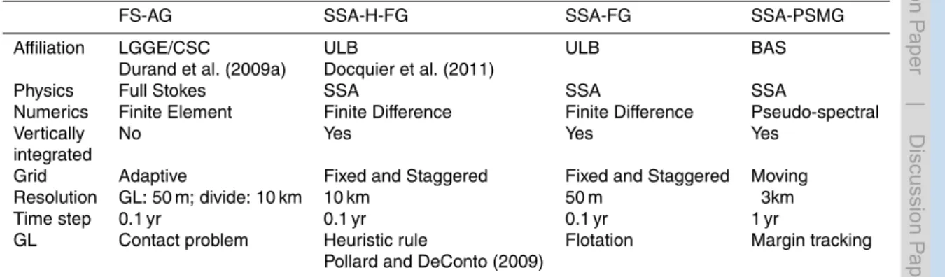
governing Stokes equations. With recent advances, one of the models deployed solves the Stokes equations, while the others solve the vertically-integrated shallow-shelf ap-proximation (SSA) (Morland, 1987; MacAyeal, 1992). The four models differ thus in the mechanical model as well as in the numerical approach used. They are briefly outlined here, with more detail to follow below.

5

The first one is the finite element full-Stokes Elmer/Ice model, denoted FS-AG for Full-Stokes – Adaptive Grid, developed at CSC/LGGE. In this application, the adaptive grid refinement proposed by Durand et al. (2009b) is used. This model is computa-tionally two dimensional in this plane-flow representation. The three remaining models solve the SSA, and are therefore vertically integrated and thus computationally

one-10

dimensional. SSA-FG (for SSA-Fixed Grid) and SSA-H-FG (for SSA-Heuristic-Fixed Grid) use a fixed grid with a resolution of 50 m and 10 km, respectively. The GL migra-tion ofSSA-H-FGis computed according to the Pollard and DeConto (2009) heuristic rule that implements the Schoof (2007) boundary condition. The last model solves the SSA equations using pseudo-spectral method (Fornberg, 1996; Hindmarsh, 2012) on

15

a moving grid, and will be denoted SSA-PSMG for SSA – Pseudo-Spectral Moving Grid. For this model, grounded ice and floating ice shelf are solved on two coupled domains, with continuity of stress and velocity across the grounding-line guaranteed. The first two models approach the problem of modelling the flow in the boundary layer by increased resolution, the third model uses a coarse resolution and a heuristic rule

20

at the GL, and the last model addresses this issue by using high-accuracy spectral methods.

Details and numerical characteristics of the four models are summarised in Table 1. In Sect. 2, specificities of the models are further described. The setup of the proposed experiments is outlined in Sect. 3 and corresponding results are discussed in Sect. 4

25

before we conclude in Sect. 5.

(6)

TCD

6, 3903–3935, 2012

A. S. Drouet et al.

Title Page

Tables Figures

◭ ◮

Back Close

Full Screen / Esc

Discussion

P

a

per

|

Dis

cussion

P

a

per

|

Discussion

P

a

per

|

Discussio

n

P

a

per

|

2 Model description

2.1 Governing equations

The problem consists of solving a gravity driven flow of incompressible and isothermal ice sliding over a rigid bedrock notedb(x). The ice is considered as a nonlinear viscous material, following the behaviour of the Glen’s flow law (Glen, 1955):

5

τ₌2ηD, (1)

where τ is the deviatoric stress tensor, D is the strain rate tensor defined as D_{i j}=

(∂jui+∂iuj)/2 andu=(u,w) is the velocity vector. The effective viscosityηis defined as follows:

η=A

−1/n

2 D

(1−n)/n

e , (2)

10

whereAand nare the Glen’s law parameter and flow law exponent respectively, and D_e is the strain-rate invariant defined asD_e2=2D_{i j}D_{i j}.

The ice flow is computed by solving the Stokes problem, expressed by the mass conservation equation in the case of incompressibility

tr (D)=div(u)=0 , (3)

15

and the linear momentum balance equation

div(σ)+ρig=0 , (4)

whereσ ₌τ−pIis the Cauchy stress tensor withp=−trσ/3 the isotropic pressure,ρ_i the ice density andgthe gravity vector.

Both the upper ice/atmosphere interface z=zs(x,t) and the lower ice/bedrock or

20

ocean interfacez=zb(x,t) are allowed to evolve following an advection equation: ∂zi

∂t +ui ∂zi

∂x −wi =ai i=s,b, (5)

(7)

TCD

6, 3903–3935, 2012

A. S. Drouet et al.

Title Page

Tables Figures

◭ ◮

Back Close

Full Screen / Esc

Discussion

P

a

per

|

Dis

cussion

P

a

per

|

Discussion

P

a

per

|

Discussio

n

P

a

per

|

where (u_i,w_i) is the surface velocity (i=s) or the basal velocity (i=b). For this appli-cation, the mass flux at the surface is constant and uniform (as(x,t)=as, see Table 2) andab=0.

2.2 Boundary conditions

The geometry is restricted to a two-dimensional plane flow along thex-direction and

5

thez-axis is the vertically upward direction. The upstream boundary of the domainx=

0 is taken to be a symmetry axis (ice divide), where we impose the horizontal velocity u(x=0)=0. The downstream boundary, x=xf corresponds to the calving front. The position of the calving frontxfis fixed, and the GL positionxgis delimited by 0≤xg≤xf. The upper ice surfacez=zs(x,t) is in contact with the atmosphere, where pressure

10

is negligible with respect to involved stresses inside the ice body. This is a stress free surface, implying the following condition:

σ·n|z_s =0 , (6)

wherenis the outward pointing unit normal vector.

The lower surfacez=zb(x,t) is either in contact with the bedrock or with the ocean,

15

and two different boundary conditions will be applied for the Stokes problem on these two different interfaces, defined as:



 

 

(

zb(x,t)> b(x) or

zb(x,t)=b(x) and −σnn|z_b≤pw

Ice/Ocean interface,

zb(x,t)=b(x) and −σnn|z_b> pw Ice/Bedrock interface.

(7)

In Eq. (7), the water pressurepw=pw(z,t) is defined as:

pw(z,t)=

(

ρwg(ℓw(t)−z) if z≤ℓw(t) 0 if z > ℓw(t)

(8)

20

(8)

TCD

6, 3903–3935, 2012

A. S. Drouet et al.

Title Page

Tables Figures

◭ ◮

Back Close

Full Screen / Esc

Discussion

P

a

per

|

Dis

cussion

P

a

per

|

Discussion

P

a

per

|

Discussio

n

P

a

per

|

whereρwis the water density andℓwis sea level, assumed constant and equal to zero in what follows.

Where the ice is in contact with the ocean (first condition in Eq. 7), the following Neumann boundary condition applies for the Stokes equations:

σ·n=−pwn. (9)

5

Where the ice is in contact with the bedrock (second condition in Eq. 7), a non-penetration condition is imposed as well as a friction law, such as

u·n₌0 , (10)

τb=t·(σ·n)|b=Cumb ,

10

whereτb is the basal shear stress, t is the tangent vector to the bedrock, ub is the sliding velocity, C is the friction parameter and m is the friction law exponent (see Table 2 for the adopted values).

2.3 Shallow shelf/shelfy stream approximation (SSA)

As mentioned previously, three of the four models use the Shallow Shelf Approximation

15

(SSA) which is a vertically integrated approximation of the Stokes Eqs. (3) and (4). The horizontal velocityu(x) is obtained by solving the following equations (Morland, 1987; MacAyeal, 1992):

(

2∂(hτxx) ∂x −Cu

m

=ρ_igh∂zs

∂x 0≤x≤xg, for the grounded part,

2∂(hτxx) ∂x =γh

∂h

∂x xg< x≤xf, for the floating part.

(11)

whereh=h(x) is the ice thickness,τxx=2η∂xuis the longitudinal deviatoric stress and

20

uis the horizontal velocity in the flow direction. The effective viscosity,η, is computed as in Eq. (2), whereD_e≈∂_xu. The parameterγis defined as:

γ=ρ_ig

1− ρi ρ_w

. (12)

(9)

TCD

6, 3903–3935, 2012

A. S. Drouet et al.

Title Page

Tables Figures

◭ ◮

Back Close

Full Screen / Esc

Discussion

P

a

per

|

Dis

cussion

P

a

per

|

Discussion

P

a

per

|

Discussio

n

P

a

per

|

According to the SSA approximation, ice deformation is dominated by membrane stresses and vertical shear within the ice is neglected. For the SSA model, the only boundary condition is u(x=0)=0 at the ice divide, whereas other boundary condi-tions are already implicitly included in the set of Eqs. (11).

The lower surfacezbis determined from the non-penetration condition and the

float-5

ing condition:

(

z_b(x,t)=b(x) forx≤x_g,

zb(x,t)=ℓw−hρi/ρw> b(x) forx > xg.

(13)

The upper surfacezs=zb+his deduced from the vertically-integrated mass conser-vation equation givinghas

∂h ∂t +

∂(hu)

∂x =as. (14)

10

2.4 Grounding line treatment

The implementation of GL treatment differs from one model to the other. In this section we define for each model the specificities regarding the treatment of the GL.

The FS-AG model solves the contact problem between the ice and the bedrock. During a time step, the contact condition (Eq. 7) is tested at each node of the mesh

15

and the bottom boundary conditions (Eq. 9) or (Eq. 10) are imposed accordingly. More details about this method and its implementation can be found in Durand et al. (2009a). The consistency of this GL implementation strongly depends on the grid resolution, and a grid size lower than 100 m is needed to obtain reliable results (Durand et al., 2009b). In order to reach this resolution while considering a reasonable number of mesh nodes,

20

an adaptive mesh refinement around the GL is applied: the horizontal distribution of nodes is updated at every time step, such that finer elements are concentrated around the GL.

(10)

TCD

6, 3903–3935, 2012

A. S. Drouet et al.

Title Page

Tables Figures

◭ ◮

Back Close

Full Screen / Esc

Discussion

P

a

per

|

Dis

cussion

P

a

per

|

Discussion

P

a

per

|

Discussio

n

P

a

per

|

For the SSA-FGmodel the grid points are kept fixed in time and the last grounded grid point is determined through the flotation criterion, i.e. by solving the following equa-tion:

F =hg− ρw

ρi

(ℓw−b(xg))=0 . (15)

The GL positionxgis given with sub-grid precision between the last grounded grid point

5

and the first floating point following the method proposed by Pattyn et al. (2006). The GL position is also determined with sub-grid precision following Pattyn et al. (2006) for theSSA-H-FG, but whileSSA-FGuses the flotation criterion as a boundary condition at the GL, theSSA-H-FGmodel makes use of an additional boundary condi-tion based on the semi-analytical solucondi-tion of Schoof (2007). The ice flux at the GLq_g

10

is calculated as a function of ice thickness at the GLhg:

qg=

Aρ_igγn 4n_C

!_m1₊₁

θmn+1h

m+n+3

m+1

g , (16)

and is used in a heuristic rule to enable GL migration (Pollard and DeConto, 2009). This parameterization allows relatively coarse resolutions to be used (10 km in this study) and gives steady-state results of GL position that are independent of the

cho-15

sen resolution and agree well with the semi-analytical solution given by Schoof (2007) (Docquier et al., 2011). In Eq. (16), the coefficient θ accounts for buttressing and is defined as

θ=

4τxx|x_g

γhg

. (17)

The numerical approach used by the pseudo-spectral SSA-PSMG model consists in

20

explicitly calculating the rate of GL migration, ˙xg, according to the following explicit

(11)

TCD

6, 3903–3935, 2012

A. S. Drouet et al.

Title Page

Tables Figures

◭ ◮

Back Close

Full Screen / Esc

Discussion

P

a

per

|

Dis

cussion

P

a

per

|

Discussion

P

a

per

|

Discussio

n

P

a

per

|

formula (Hindmarsh and LeMeur, 2001)

˙ xg=−

∂_tF ∂xF

, (18)

whereF is given by Eq. (15). At each time step, a new position is computed and the grid moves accordingly, so that the GL coincides exactly with a grid point (Hindmarsh, 1993). Moving grids have the ability to ensure that a grid-point always coincides with

5

the GL, allowing easy representation of gradients at this location but, are not always convenient to implement.

2.5 Calving front boundary condition and the specification of buttressing

The experiments we propose are driven by changes in the buttressing force. One ap-proach could have consisted of applying lateral friction on the ice-shelf following the

10

method of Gagliardini et al. (2010), but the total buttressing force would then have been function of the ice-shelf area and ice-shelf velocities, and therefore different for all models. In order to ensure the same buttressing force for all models, we follow the method proposed by Price et al. (2011), in which the inward force at the calving front is modified by a factor, notedCF in our study.

15

For vertically integrated models, the horizontal force acting on the calving front is entirely due to the hydrostatic water pressure and the longitudinal deviatoric stress at the front is given by (MacAyeal et al., 1996):

τxx|x_f= γ

4hf, (19)

wherehf is the ice thickness at the calving front. In the case of the vertically integrated

20

modelsSSA-FG,SSA-H-FG andSSA-PSMG, a factorCF is then used to modify lon-gitudinal deviatoric stress (Eq. 19), which becomes:

τ_xx|x_f=CF γ

4hf. (20)

(12)

TCD

6, 3903–3935, 2012

A. S. Drouet et al.

Title Page

Tables Figures

◭ ◮

Back Close

Full Screen / Esc

Discussion

P

a

per

|

Dis

cussion

P

a

per

|

Discussion

P

a

per

|

Discussio

n

P

a

per

|

A value of C_F = 1 means that the longitudinal deviatoric stress at the calving front implies that ice extension is opposed solely by water pressure, corresponding to no buttressing. Values less than one induce a lower extensional longitudinal deviatoric stress at the front, simulating the effect of buttressing. Note that this procedure implies an additionalforceapplied at the calving front; this results in a varyingstressupstream

5

as the ice thickens.

Moreover, for SSA-H-FG, the buttressing parameter C_F is by construction incorpo-rated in the boundary condition at the GL. This boundary condition relates the ice flux qg to the ice thickness hg at the GL and includes the buttressing factor θ as defined by Eq. (17). From the SSA equations in the ice shelf, we derive (see Appendix A) the

10

relation that linksθ and CF through both the ice thickness at the GL hg and the ice thickness at the calving fronthf:

θ=1−(1−C_F) hf hg

!2

. (21)

The other two SSA models solve for the longitudinal variation of τxx in the shelf to compute the value at the grounding-line.

15

For the FS-AGmodel, the hydrostatic pressure pw(z) is imposed along the ice col-umn in contact with the sea, so that the longitudinal Cauchy stress is not uniform on this boundary. This non-uniform stress induces a bending of the ice-shelf near the front. To avoid an increase of this bending when adding the buttressing, the stress condition at the front is modified by adding a uniform buttressing stresspb, such that

20

σxx|x_f(z,t)=pw(z)+pb(t) . (22)

Using Eqs. (22) and (20), and assuming the equality of the mean longitudinal Cauchy stress for both parameterisations, the buttressing stress to be apply at the front of the full-Stokes model is obtained as a function ofC_F (see Appendix B), such as

pb= ρwgz

2 b 2ρ_ihf

(ρw−ρi)(CF −1) . (23)

25

(13)

TCD

6, 3903–3935, 2012

A. S. Drouet et al.

Title Page

Tables Figures

◭ ◮

Back Close

Full Screen / Esc

Discussion

P

a

per

|

Dis

cussion

P

a

per

|

Discussion

P

a

per

|

Discussio

n

P

a

per

|

Note thatpbhas to be computed at each time step since it depends on the ice thickness at the front, which is not constant.

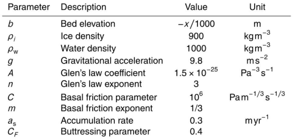
3 Experimental setup

We consider an ice sheet resting on a downward sloping bedrock, with the calving front fixed at 1000 km. The GL never advances as far as this in the experiments. The flow

pa-5

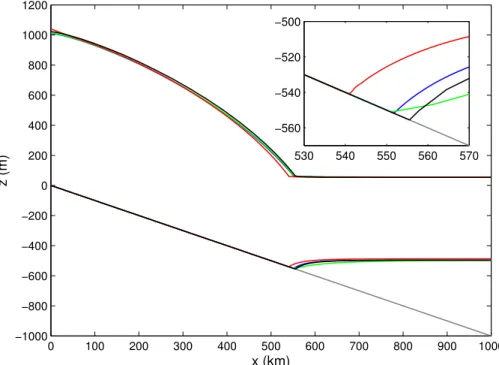
rameters summarised in Table 2 are used by each model in order to calculate a steady state geometry. The steady state is obtained with a buttressed ice-shelf (C_F =0.4). Computed steady surfaces are in good agreement between models, exhibiting only a slight difference in GL position of less than 20 km (see Fig. 1). We chose the simpler, stable case of a forward slope for the simple reason that computing comparable initial

10

starting conditions on the unstable reverse slope is a practical impossibility. Grounding-line retreat rates are governed by the water depth and the buttressing, and we chose values that were physically acceptable and also produced physically reasonable retreat rates.

Ice-sheet geometry is subsequently perturbed by a release of the initial buttressing

15

force. This process, arising from increased melt of the ice shelf, appears to be respon-sible for the observed acceleration of Antarctic outlet glacier (Pritchard et al., 2012). Starting from the steady geometries obtained with initial factorCF =0.4, the buttressing force is decreased att=0 ( i.e.C_F increases) and kept constant during the simulation. Since we focus on the transient behaviour, simulations are run during 200 yr. Three

20

different amplitudes of the perturbation are investigated with corresponding modified values ofC_F =0.5, 0.8 and 1.

(14)

TCD

6, 3903–3935, 2012

A. S. Drouet et al.

Title Page

Tables Figures

◭ ◮

Back Close

Full Screen / Esc

Discussion

P

a

per

|

Dis

cussion

P

a

per

|

Discussion

P

a

per

|

Discussio

n

P

a

per

|

4 Results and discussion

4.1 Transient behaviour of direct observable variables on actual ice sheets

We first evaluate the response of the various models regarding the variables that are currently observed over actual ice sheets, namely GL position (Fig. 2), surface elevation change (Fig. 3) and surface velocities (Fig. 4).

5

As expected, release of buttressing induces a GL retreat, and the greater the re-lease, the higher the amount and rate of retreat (Gagliardini et al., 2010). Retreat can reach up to almost 100 km in 200 yr following a complete loss of buttressing restraint (CF =1, see Fig. 2 and Table 3). The different models show a similar trend regarding the temporal evolution of GL position (left panels in Fig. 2). However, owing to the

var-10

ious initial steady state profiles, the GL position differs between models. For the three perturbations, SSA-H-FG shows the highest GL retreat compared to the initial posi-tion, followed bySSA-FG, thenSSA-PSMG, and finallyFS-AG(Table 3). The evolution of the GL position ofSSA-H-FG has a step-like behaviour due to the model grid size (10 km).

15

Rates of GL migration (right panels in Fig. 2) for SSA-PSMG and SSA-FG exhibit a very similar pattern, i.e. a high retreat rate value in the beginning of the perturbation and then a convergence towards a zero-value. Moreover, the greater the perturbation (higher value ofCF), the higher the retreat rates in the beginning of the perturbation. The smooth decrease of the migration rate computed bySSA-PSMGis due to the

ex-20

plicit way the GL migration is computed (see model description above). Because the

SSA-FG interpolates the GL position between the last grounded point and the first floating point (Pattyn et al., 2006), it also ensures a smooth description of GL migration rate. However,FS-AGand SSA-H-FGshow discontinuous GL migration rate induced by numerical artefacts: both models give results that are affected by their grid size. The

25

stepped patterns obtained withFS-AGare due to high frequency oscillation between two successive nodes during GL migration: the GL retreats, then stays at the same position during one time step, then retreats, etc. so that the GL migration rate oscillates

(15)

TCD

6, 3903–3935, 2012

A. S. Drouet et al.

Title Page

Tables Figures

◭ ◮

Back Close

Full Screen / Esc

Discussion

P

a

per

|

Dis

cussion

P

a

per

|

Discussion

P

a

per

|

Discussio

n

P

a

per

|

with an amplitude of 500 m yr−1(i.e. grid size divided by time step). The numerical noise found inSSA-H-FGis due to a combination of both the grid size effect and single-cell dithering (Pollard and DeConto, 2012). As a general trend, the GL retreats by 10 km steps as a consequence of the model resolution (grid size effect). At some discrete GL positions (every 10 km), the rate of GL migration varies significantly due to the

heuris-5

tic rule used in the model (flux imposed either upstream or downstream the GL), so that the GL slightly advances and retreats within the same grid cell (single-cell dither-ing). In summary, the GL retreats by 10 km (corresponding to the model resolution) and reaches a discrete position where it oscillates within the same grid cell, and then retreats before reaching another discrete position again, etc.

10

Rates of surface elevation change through time and distance from the ice divide are presented in Fig. 3 for the various models and perturbations. The horizontal velocity on the surface velocity is similarly plotted (see Fig. 4). The largest perturbation (C_F =1) exhibits rates of surface elevation change of a few meters per year in the beginning, with horizontal velocities above one kilometer per year. Together with GL migration

15

rates of the order of a kilometer per year (Fig. 2), those are in general agreement with the obervation for currently recessing glaciers of West Antarctica, and Pine Island Glacier in particular (Rignot, 1998; Rignot et al., 2011). That confirms the relevance of the amplitude of the perturbations applied. Rates of surface elevation change are quite similar between the four models (Fig. 3). The highest thinning rates appear in the

20

vicinity of the GL at the beginning of the perturbation. Similarly, the surface velocities steadily decrease during the simulation (Fig. 4). High frequency and small amplitude numerical noise inFS-AGappear not to significantly affect the surface response. How-ever, with SSA-H-FG the high frequency and amplitude variabilities drastically affect the surface thinning rate and velocities over short time scales (i.e. about a decade).

25

We deliberately chose a low spatial resolution (uniform 10 km along the flowline) for theSSA-H-FG model compared with other models. As shown by Docquier et al. (2011), such models perform well at low spatial resolution, which is the main motivation for applying such parameterizations in large-scale ice sheet models. Increasing the

(16)

TCD

6, 3903–3935, 2012

A. S. Drouet et al.

Title Page

Tables Figures

◭ ◮

Back Close

Full Screen / Esc

Discussion

P

a

per

|

Dis

cussion

P

a

per

|

Discussion

P

a

per

|

Discussio

n

P

a

per

|

resolution (down to 250 m) allows removal of high frequency numerical artefacts and a better match to the three other models (data not shown). However, this significantly increases its numerical cost, so that the major advantage of this model is lost, as well as its applicability to large-scale ice-sheet models.

4.2 Divergence from the boundary-layer solution

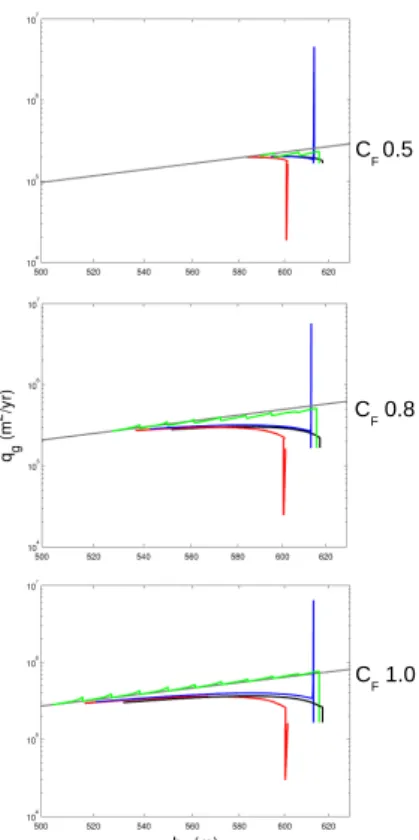
5

Despite the numerical noise exhibited by SSA-H-FG and FS-AG models, the evolu-tion of the geometry during the simulaevolu-tions appears very similar for all four models. However, the boundary layer theory implemented in the SSA-H-FG model hypothe-sizes near-steady conditions and its ability to represent transients requires evaluation. In Fig. 5, the flux at the GL is plotted as a function of the instantaneous ice

thick-10

ness at the GL for all models and simulations. By construction,SSA-H-FG essentially follows the boundary layer prescription. This can most clearly be seen for the case C_F =1 (see the bottom of Fig. 5) where the close correspondence of the curves of Schoof (2007) and SSA-H-FG is evident. This correspondence is not evident for the other perturbations, since theSSA-H-FGboundary condition for the flux now relies on

15

a parameterization of θ, which in turn depends on the quantity hf/hg (see Eq. 21). Since this ratio varies in time, the steady-state condition of the Schoof condition is not fulfilled.

Interestingly, and despite their very different physical and numerical approaches, all the other models show very similar behaviour, with the boundary layer theory result

20

attained after some time. This is most obvious for the largest perturbation (CF =1) but also clearly visible for the weaker perturbations (CF =0.8 and 0.5). However, during the highly transient phase, for a given ice thickness at the GL, the ice flux is substantially overestimated by the boundary layer theory, consequently overestimating the outflow during the whole period of 200 yr.

25

(17)

TCD

6, 3903–3935, 2012

A. S. Drouet et al.

Title Page

Tables Figures

◭ ◮

Back Close

Full Screen / Esc

Discussion

P

a

per

|

Dis

cussion

P

a

per

|

Discussion

P

a

per

|

Discussio

n

P

a

per

|

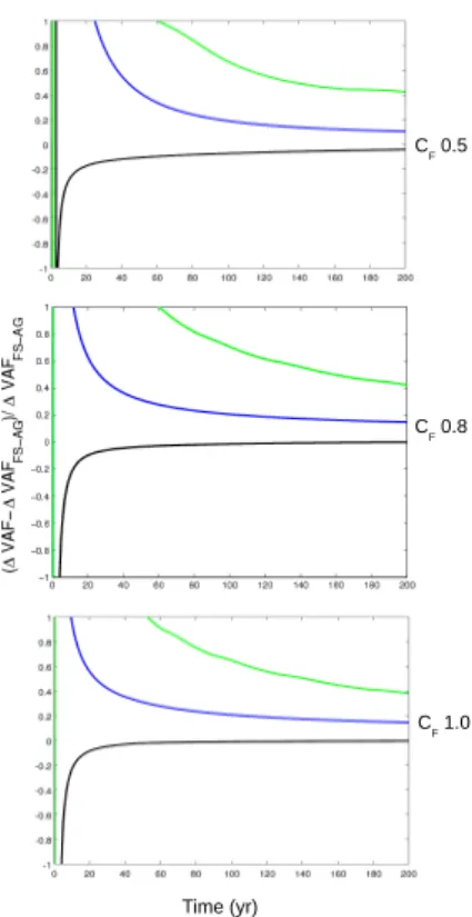
4.3 Changes in Volume Above Flotation (∆VAF)

From the perspective of projecting the future contribution of Antarctica to sea level rise, the change in Volume Above Flotation (∆VAF=VAF(t)−VAF(t=0)) is certainly a per-tinent variable to investigate. Indeed,∆VAF has the advantage of integrating through time both the contribution coming from outflow at the GL and the consequence of

5

grounding-line retreat in terms of ice release. In our case, this further allows inves-tigating the spread in the transient behaviour of the various models in response to similar perturbations. We arbitrary choose to express the evolution of∆VAF for each model relative to∆VAF computed byFS-AG. Corresponding evolutions are presented in Fig. 6. It is first of all striking that response in terms of relative_∆VAF from one model

10

to the others are extremely similar, irrespective of the amplitude of the perturbation. As anticipated, SSA-H-FG shows the greatest change in VAF compared with other models. Relative toFS-AG,SSA-H-FG overestimates the contribution to SLR by more than 100 % during the first 50 yr of the simulation, which decreases to a 40 % over-estimation after 200 yr.SSA-FGshows a similar pattern with a smaller overestimation

15

(about 15 % after 200 yr). On the other hand,SSA-PSMG briefly underestimates the change in VAF relative to FS-AGat the beginning of the perturbation, but after 20 yr the contribution of the models to SLR is remarkably similar to the one computed by

FS-AG, with relative di_fference below 5 %. While this intercomparison has not given definitive values for the GL migration rates, it strongly suggests that models

prescrib-20

ing flux at the GL according to the boundary layer theory most probably overestimate ice discharge. It also clearly shows that the rate of contribution to SLR significantly differs from one model to the other, even for a relatively simple and constrained ex-periment. When extrapolated to the current imbalance of the Antarctic ice sheet, this would have important consequences. According to Rignot et al. (2011), the Antarctic

25

ice sheet drained about 100 Gt yr−1 in 2000 with an increasing acceleration trend in mass loss of 14.5 Gt yr−2. Following that trend, the Antarctic ice sheet have contributed by 4.6 mm of SLR between 2000 and 2010. Assuming that ice-sheet models were

(18)

TCD

6, 3903–3935, 2012

A. S. Drouet et al.

Title Page

Tables Figures

◭ ◮

Back Close

Full Screen / Esc

Discussion

P

a

per

|

Dis

cussion

P

a

per

|

Discussion

P

a

per

|

Discussio

n

P

a

per

|

capable of describing exactly the ice dynamical conditions in 2000, and also assuming the parameters forcing enhanced ice discharge to be properly known, the above uncer-tainties in modelled ice discharge would lead to a erroeneous contribution between 3.1 and 18 mm in 2010, due to the over-estimation ofSSA-H-FGof more than 300 % in the first 10 yr after a given perturbation. Furthermore, as ice sheets are still in a transient

5

phase (i.e., perturbations are sustained through time) the discrepancy of the models would eventually increase with time integration. Of course, these assertions have to be moderated by the fact that the complexity of actual 3-D geometries could mitigate the discrepancy between model results, which is the focus of future research.

5 Conclusions

10

We have computed the transient response of four flow-line ice-sheet models to a re-duction in the buttressing force exerted by an ice shelf onto the upstream grounded ice sheet. The intensity of buttressing perturbations was chosen in order to reproduce changes in geometry that are comparable to those observed on current ice sheets. Compared with MISMIP, we investigated the transient response in more detail and

ap-15

plied a perturbation that reflects direct mechanical forcing.

The physics are implemented in a di_fferent way in the di_fferent models (from SSA to the solution of the full-Stokes equations), while the models differ in their numerical treatment as well (finite difference and finite element). One of the models includes the heuristic rule of Pollard and DeConto (2009), i.e. the flux-thickness relation proposed

20

by Schoof (2007) is imposed at the GL. All models have successfully participated in the MISMIP benchmark (Pattyn et al., 2012), exhibiting unique stable positions on down-ward sloping beds, unstable GL positions on retrograde slopes and related hysteresis behaviour over an undulated bedrock.

Surprisingly, and despite the different physics and numerics implemented, all models

25

give consistent results in terms of change in surface geometry and migration of the GL. A major divergence is found with theSSA-H-FG model which directly implements the

(19)

TCD

6, 3903–3935, 2012

A. S. Drouet et al.

Title Page

Tables Figures

◭ ◮

Back Close

Full Screen / Esc

Discussion

P

a

per

|

Dis

cussion

P

a

per

|

Discussion

P

a

per

|

Discussio

n

P

a

per

|

boundary layer theory proposed by Schoof (2007). Here, the prescription of flux at the GL introduces high frequency, large amplitude numerical noise deteriorating the surface change signal over decadal time scales. Moreover, it seems that at least in these experiments that the boundary layer theory overestimates the discharge during the transient evolution. As a consequence, models that prescribe the flux at the GL

5

should be used with particular caution when dealing with small spatial and temporal scales.

Estimation of the contribution to SLR through numerical modelling still exhibits large uncertainties, with results from different models showing>100 % spread on a decadal time-scale and still around 40 % two hundred years after the initial change in

buttress-10

ing. There may be a large uncertainty in models that are seeking to establish reliable projection of coming contribution of Antarctic ice sheet to SLR. Further model inter-comparison must be pursued to better constrain the rate of discharge, and intercom-parisons on specific Antarctic outlet glaciers should be encouraged in the near future.

Appendix A

15

In this Appendix the relation between the buttressing factorsθ in Eq. (17) and CF in Eq. (20) is derived. The ice-shelf equation is

2∂(hτxx) ∂x =

γ 2

∂(h2)

∂x , (A1)

wherehis the ice thickness along the ice-shelf. The longitudinal deviatoric stress within the ice shelf is then obtained as

20

τ_xx=γ

4h− B

h, (A2)

(20)

TCD

6, 3903–3935, 2012

A. S. Drouet et al.

Title Page

Tables Figures

◭ ◮

Back Close

Full Screen / Esc

Discussion

P

a

per

|

Dis

cussion

P

a

per

|

Discussion

P

a

per

|

Discussio

n

P

a

per

|

where B is the back-force at the calving front. Evaluatting this at x=xf and using (Eq. 20), we obtain

τxx|x_f=CF γ 4hf=

γ 4hf−

B hf

, (A3)

yielding

B=(1−C_F)γ 4h

2

f , (A4)

5

and

τ_xx=γ

4 h−(1−CF) h2_f

h

!

. (A5)

Now, at the GLx=xg, by definition ofθ(Eq. 17):

τ_xx|xg=θ

γ

4hg, (A6)

so that

10

θ=1−(1−CF) hf hg

!2

. (A7)

Appendix B

In this appendix, we demonstrate how is obtained the buttressing pressure pb(t) in Eq. (22) giving the front-stress for theFS-AGmodel. We need to findpb(t) such that the

(21)

TCD

6, 3903–3935, 2012

A. S. Drouet et al.

Title Page

Tables Figures

◭ ◮

Back Close

Full Screen / Esc

Discussion

P

a

per

|

Dis

cussion

P

a

per

|

Discussion

P

a

per

|

Discussio

n

P

a

per

|

mean longitudinal Cauchy stress be the same for all models. This equality is expressed as follows:

¯

σ_xxSSA=σ¯_xxF S (B1)

where ¯σxxSSA and ¯σxxF S are the longitudinal Cauchy stress of SSA models and FS-AG model,=respectively.

5

The mean longitudinal Cauchy stress for SSA models reads:

¯

σ_xxSSA=2 ¯τxx+σ¯zz (B2)

where ¯σ_zz=−ρighf

2 and ¯τxx is given by Eq. (20).

The longitudinal Cauchy stress for FS-AGmodel, given by Eq. (22), and once inte-grated over the ice column gives:

10

¯

σ_xxF S =−ρwgzb 2

2hf

+pb (B3)

Using Eq. (B2) for SSA models and Eq. (B3) forFS-AG, Eq. (B1) leads to

2C_Fγ 4hf−

ρighf

2 =−

ρwgzb 2

2hf

+pb (B4)

Using the flotation conditionρihf=ρwzb, and after simplifications, pb can be isolated and deduced as

15

pb= ρwgz

2 b 2ρ_ihf

(ρw−ρi)(CF −1) . (B5)

Acknowledgements. Some of the computations presented in this paper were performed using the CIMENT infrastructure (https://ciment.ujf-grenoble.fr), which is supported by the Rh ˆone-Alpes region (GRANTCP E R07₁3 CIRA: http://www.ci-ra.org). This work was also supported

(22)

TCD

6, 3903–3935, 2012

A. S. Drouet et al.

Title Page

Tables Figures

◭ ◮

Back Close

Full Screen / Esc

Discussion

P

a

per

|

Dis

cussion

P

a

per

|

Discussion

P

a

per

|

Discussio

n

P

a

per

|

by funding from the ice2sea programme from the European Union 7th Framework Programme, grant number 226375. Ice2sea contribution number 127.

The publication of this article is financed by CNRS-INSU. 5

References

Docquier, D., Perichon, L., and Pattyn, F.: Representing grounding line dynamics in nu-merical ice sheet models: recent advances and outlook, Surv. Geophys., 32, 417–435, doi:10.1007/s10712-011-9133-3, 2011. 3912, 3917, 3927

Durand, G., Gagliardini, O., de Fleurian, B., Zwinger, T., and Meur, E. L.: Marine ice 10

sheet dynamics: hysteresis and neutral equilibrium, J. Geophys. Res., 114, F03009, doi:10.1029/2008JF001170, 2009a. 3911, 3927

Durand, G., Gagliardini, O., Zwinger, T., Meur, E. L., and Hindmarsh, R.: Full-Stokes modeling of marine ice sheets: influence of the grid size, Ann. Glaciol., 50, 109–114, 2009b. 3907, 3911

15

Fornberg, B.: A Practical Guide to Pseudospectral Methods, Cambridge University Press, Cam-bridge, United Kingdom, 1996. 3907

Gagliardini, O., Durand, G., Zwinger, T., Hindmarsh, R., and Meur, E. L.: Coupling of ice-shelf melting and buttressing is a key process in ice-sheets dynamics, Geophys. Res. Lett., 37, L14501, doi:10.1029/2010GL043334, 2010. 3913, 3916

20

Gillet-Chaulet, F. and Durand, G.: Glaciology: ice sheet advance in Antarctica, Nature, 467, 794–795, 2010. 3905

Glen, J.: The creep of polycristalline ice, P. R. Soc. A, 228, 519–538, 1955. 3908

Hindmarsh, R.: Qualitative dynamics of marine ice sheets, in: Ice in the Climate System, edited by Peltier, W. R., Springer-Verlag, Berlin, 68–99, 1993. 3913

25

(23)

TCD

6, 3903–3935, 2012

A. S. Drouet et al.

Title Page

Tables Figures

◭ ◮

Back Close

Full Screen / Esc

Discussion

P

a

per

|

Dis

cussion

P

a

per

|

Discussion

P

a

per

|

Discussio

n

P

a

per

|

Hindmarsh, R.: An observationally validated theory of viscous flow dynamics at the ice-shelf calving front, J. Glaciol., 58, 375–387, 2012. 3907

Hindmarsh, R. and LeMeur, E.: Dynamical processes involved in the retreat of marine ice sheets, J. Glaciol., 47, 271–282, 157, 2001. 3913

Larour, E., Schiermeier, J., Rignot, E., Seroussi, H., Morlighem, M., and Paden, M.: Sensitivity 5

analysis of Pine Island Glacier ice flow using ISSM and DAKOTA, J. Geophys. Res., 117, F02009, doi:10.1029/2011JF002146, 2012. 3905

MacAyeal, D.: Irregular oscillations of the West Antarctic ice sheet, Nature, 365, 214–215, 1992. 3907, 3910

MacAyeal, D., Hulbe, C., Huybrechts, P., Rommelaere, V., Determann, J., and Ritz, C.: An ice-10

shelf model test based on the Ross ice shelf, Ann. Glaciol., 365, 46–51, 1996. 3913

Morland, L.: Unconfined ice shelf flow, in: Dynamics of the West Antarctic Ice Sheet, edited by: der Veen, C. J. V. and Oerlemans, J., Cambridge University Press, UK and New York, NY, USA, 1987. 3907, 3910

Morlighem, M., Rignot, E., Seroussi, H., Larour, E., Dhia, H. B., and Aubry, D.: Spatial patterns 15

of basal drag inferred using control methods from a full-Stokesusing control methods from and simpler models for Pine Island glacier, West Antarctica, Geophys. Res. Lett., 37, L14502, doi:10.1029/2010GL043853, 2010. 3905

Nick, F. M., Vieli, A., Howat, I. M., and Joughin, I.: Large-scale changes in Greenland outlet glacier dynamics triggered at the terminus, Nat. Geosci., 2, 110–114, doi:10.1038/ngeo394, 20

2009. 3906

Pattyn, F., Huyghe, A., Brabander, S., and Smedt, B. D.: Role of transition zones in marine ice sheet dynamics, J. Geophys. Res., 111, F02004, doi:10.1029/2005JF000, 2006. 3912, 3916 Pattyn, F., Schoof, C., Perichon, L., Hindmarsh, R. C. A., Bueler, E., de Fleurian, B., Durand, G., Gagliardini, O., Gladstone, R., Goldberg, D., Gudmundsson, G. H., Huybrechts, P., Lee, V., 25

Nick, F. M., Payne, A. J., Pollard, D., Rybak, O., Saito, F., and Vieli, A.: Results of the Marine Ice Sheet Model Intercomparison Project, MISMIP, The Cryosphere, 6, 573–588, doi:10.5194/tc-6-573-2012, 2012. 3905, 3920

Pollard, D. and DeConto, R.: Modelling West Antarctic ice sheet growth and collapse through the past five million years, Nature, 458, doi:10/1038/nature07809, 2009. 3907, 3912, 3920, 30

3927

(24)

TCD

6, 3903–3935, 2012

A. S. Drouet et al.

Title Page

Tables Figures

◭ ◮

Back Close

Full Screen / Esc

Discussion

P

a

per

|

Dis

cussion

P

a

per

|

Discussion

P

a

per

|

Discussio

n

P

a

per

|

Pollard, D. and DeConto, R. M.: Description of a hybrid ice sheet-shelf model, and application to Antarctica, Geosci. Model Dev. Discuss., 5, 1077–1134, doi:10.5194/gmdd-5-1077-2012, 2012. 3917

Price, S. I., Howat, A. P., and Smith, B.: Committed sea-level rise for the next century from Greenland ice sheet dynamics during the past decade, P. Natl. Acad. Sci. USA, 108, 8978– 5

8983, 2011. 3906, 3913

Pritchard, H. D., Ligtenberg, S., Fricker, H., Vaughan, D., Van den Broeke, M., and Padman, L.: Antarctic ice-sheet loss driven by basal melting of ice shelves, Nature, 484, 202–205, 2012. 3904, 3915

Rignot, E.: Fast recession of a West Antarctic glacier, Science, 281, 549–551, 1998. 3917 10

Rignot, E., Bamber, J. L., van den Broeke, M. R., Davis, C., Li, Y., van de Berg, W. J., and van Meijgaard, E.: Recent Antarctic ice mass loss from radar interferometry and regional climate modelling, Nat. Geosci., 1, 106–110, doi:10.1038/ngeo102, 2008. 3904

Rignot, E., Velicogna, I., van den Broeke, M. R., Monaghan, A., and Lenaerts, J.: Acceleration of the contribution of the Greenland and Antarctic ice sheets to sea level rise, Geophys. Res. 15

Lett., 38, L05503, doi:doi:10.1029/2011GL046583, 2011. 3904, 3917, 3919

Schoof, C.: Ice sheet grounding line dynamics: steady states, stability, and hysteresis, J. Geo-phys. Res., F03S28, doi:10.1029/2006JF000664, 2007. 3905, 3906, 3907, 3912, 3918, 3920, 3921, 3934

Velicogna, I.: Increasing rates of ice mass loss from the Greenland and Antarctic Ice Sheet 20

revealed from GRACE, J. Geophys. Res., 36, L19503, doi:10.1029/2009GL040222, 2009. 3904

Vieli, A. and Payne, A.: Assessing the ability of numerical ice sheet models to simulate ground-ing line migration, J. Geophys. Res., 110, F01003, doi:10.1029/2004JF000202, 2005. 3905 Weertman, J.: Stability of a junction of an ice sheet and an ice shelf, J. Glaciol., 13, 3–11, 1974. 25

3905

Williams, C., Hindmarsh, R. C. A., and Arthern, R.: Frequency response of ice streams, P. Roy. Soc. A, doi:10.1098/rspa.2012.0180, 2012. 3906

Wingham, D., Shepherd, A., Muir, A., and Marshall, J.: Mass balance of the Antarctic ice sheet, Philos. T. R. Soc. A, 364, 1627–1635, doi:10.1098/rsta.2006.1792, 2006. 3904

30

(25)

TCD

6, 3903–3935, 2012

A. S. Drouet et al.

Title Page

Tables Figures

◭ ◮

Back Close

Full Screen / Esc

Discussion

P

a

per

|

Dis

cussion

P

a

per

|

Discussion

P

a

per

|

Discussio

n

P

a

per

|

Table 1.Summary table of model characteristics.

FS-AG SSA-H-FG SSA-FG SSA-PSMG Affiliation LGGE/CSC ULB ULB BAS

Durand et al. (2009a) Docquier et al. (2011)

Physics Full Stokes SSA SSA SSA

Numerics Finite Element Finite Difference Finite Difference Pseudo-spectral Vertically No Yes Yes Yes

integrated

Grid Adaptive Fixed and Staggered Fixed and Staggered Moving Resolution GL: 50 m; divide: 10 km 10 km 50 m 3km Time step 0.1 yr 0.1 yr 0.1 yr 1 yr

GL Contact problem Heuristic rule Flotation Margin tracking Pollard and DeConto (2009)

(26)

TCD

6, 3903–3935, 2012

A. S. Drouet et al.

Title Page

Tables Figures

◭ ◮

Back Close

Full Screen / Esc

Discussion

P

a

per

|

Dis

cussion

P

a

per

|

Discussion

P

a

per

|

Discussio

n

P

a

per

|

Table 2.Parameters of initial steady state.

Parameter Description Value Unit

b Bed elevation −x/1000 m

ρ_i Ice density 900 kg m−3

ρ_w Water density 1000 kg m−3

g Gravitational acceleration 9.8 m s−2

A Glen’s law coe_fficient 1.5×10−25 Pa−3s−1

n Glen’s law exponent 3

C Basal friction parameter 106 Pa m−1/3s−1/3

m Basal friction exponent 1/3

a_s Accumulation rate 0.3 m yr−1

C_F Buttressing parameter 0.4

(27)

TCD

6, 3903–3935, 2012

A. S. Drouet et al.

Title Page

Tables Figures

◭ ◮

Back Close

Full Screen / Esc

Discussion

P

a

per

|

Dis

cussion

P

a

per

|

Discussion

P

a

per

|

Discussio

n

P

a

per

|

Table 3.GL position for the intial steady state (C_F =0.4) and for the different perturbations for each model after 200 yr. The difference between the initial steady state and the perturbed state is given in brackets. All values are in km.

FS-AG SSA-FG SSA-H-FG SSA-PSMG

C_F =0.4 540.5 551.8 554.1 556.1

C_F =0.5 523.8 (16.7) 534.7 (17.1) 530.4 (23.8) 539.2 (16.9)

C_F =0.8 482.0 (58.5) 488.5 (63.3) 474.8 (79.3) 495.2 (60.9)

C_F =1 463.7 (76.8) 468.9 (82.9) 454.3 (99.8) 476.8 (79.3)

(28)

TCD

6, 3903–3935, 2012

A. S. Drouet et al.

Title Page

Tables Figures

◭ ◮

Back Close

Full Screen / Esc

Discussion

P

a

per

|

Dis

cussion

P

a

per

|

Discussion

P

a

per

|

Discussio

n

P

a

per

|

0 100 200 300 400 500 600 700 800 900 1000

−1000 −800 −600 −400 −200 0 200 400 600 800 1000 1200

x (km)

z (m)

530 540 550 560 570

−560 −540 −520 −500

Fig. 1.Initial steady state geometry (C_F =0.4) for all models:FS-AG in red,SSA-FGin blue,

SSA-H-FG in green and SSA-PSMG in black. The inset emphasizes the differences in GL position.

(29)

TCD

6, 3903–3935, 2012

A. S. Drouet et al.

Title Page

Tables Figures

◭ ◮

Back Close

Full Screen / Esc

Discussion

P

a

per

|

Dis

cussion

P

a

per

|

Discussion

P

a

per

|

Discussio

n

P

a

per

|

C

F 1.0

C

F 0.5

C

F 0.8

Fig. 2.Grounding line positionx_g(left) and migration ratedx_g/d t(right) as a function of time for the three buttressing values (C_F =0.5,C_F =0.8 andC_F =1), and for the four models (FS-AG

in red,SSA-FGin blue,SSA-H-FGin green andSSA-PSMGin black).

(30)

TCD

6, 3903–3935, 2012

A. S. Drouet et al.

Title Page

Tables Figures

◭ ◮

Back Close

Full Screen / Esc

Discussion

P

a

per

|

Dis

cussion

P

a

per

|

Discussion

P

a

per

|

Discussio

n

P

a

per

|

X (km)

C_F 1.0

C_F 0.5

C_F 0.8

Fig. 3.Rate of surface elevation change (m yr−1) as a function of time and horizontal distance (x=0 corresponds to the ice divide andx_f=1000 km is the calving front) for the three buttress-ing values and for the four models.

(31)

TCD

6, 3903–3935, 2012

A. S. Drouet et al.

Title Page

Tables Figures

◭ ◮

Back Close

Full Screen / Esc

Discussion

P

a

per

|

Dis

cussion

P

a

per

|

Discussion

P

a

per

|

Discussio

n

P

a

per

|

X(km)

C_F0.5

C_F 0.8

C_F 1.0

Fig. 4.Surface horizontal velocity (m yr−1) as a function of time and horizontal distance (x=0 corresponds to the ice divide andxf=1000 km is the calving front) for the three buttressing values and for the four models.

(32)

TCD

6, 3903–3935, 2012

A. S. Drouet et al.

Title Page

Tables Figures

◭ ◮

Back Close

Full Screen / Esc

Discussion

P

a

per

|

Dis

cussion

P

a

per

|

Discussion

P

a

per

|

Discussio

n

P

a

per

|

C F 1.0 C

F 0.8 C

F 0.5

Fig. 5. GL ice flux q_g as a function of GL ice thickness h_g for the four models (FS-AG in

red,SSA-FGin blue,SSA-H-FG in green andSSA-PSMGin black) and for the three different buttressing values, compared with the Schoof (2007) solution (in grey).

(33)

TCD

6, 3903–3935, 2012

A. S. Drouet et al.

Title Page

Tables Figures

◭ ◮

Back Close

Full Screen / Esc

Discussion

P

a

per

|

Dis

cussion

P

a

per

|

Discussion

P

a

per

|

Discussio

n

P

a

per

|

C

F 1.0

C

F

0.8 C

F 0.5

ime (yr)

Fig. 6.Temporal evolution of the variation of Volume above Flotation (_∆VAF), expressed relative toFS-AG (∆VAF_FS-AG) for the three remaining models (SSA-FG in blue,SSA-H-FG in green andSSA-PSMGin black).