www.ann-geophys.net/33/703/2015/ doi:10.5194/angeo-33-703-2015
© Author(s) 2015. CC Attribution 3.0 License.
Equation of state for solar near-surface convection
N. Vitas1,2and E. Khomenko1,2,3
1Instituto de Astrofísica de Canarias, C/ Via Lactea S/N, 38200 La Laguna, Tenerife, Spain 2Universidad de La Laguna, Dpto. Astrofísica, 38206 La Laguna, Tenerife, Spain
3Main Astronomical Observatory, Academy of Sciences Ukraine, Golosiiv, Kiev 22, 252650, Ukraine
Correspondence to:N. Vitas ([email protected])
Received: 27 August 2014 – Revised: 17 March 2015 – Accepted: 29 March 2015 – Published: 9 June 2015
Abstract.Numerical 3-D radiative hydrodynamical simula-tions are the main tool for the analysis of the interface be-tween the solar convection zone and the photosphere. The equation of state is one of the necessary ingredients of these simulations. We compare two equations of state that are com-monly used, one ideal and one nonideal, and quantify their differences. Using a numerical code we explore how these differences propagate with time in a 2-D convection sim-ulation. We show that the runs with different equations of state (EOSs) and everything else identical relax to statisti-cally steady states in which the mean temperature (in the range of the continuum optical depths typical for the solar photosphere) differs by less than 0.2 %. For most applica-tions this difference may be considered insignificant. Keywords. Solar physics astrophysics and astronomy (pho-tosphere and chromosphere)
1 Introduction
Realistic time-dependent 3-D numerical simulations (Nord-lund, 1982; Stein and Nord(Nord-lund, 1998, 2000) radically im-proved our knowledge of the near-surface convection and the solar photosphere. In these simulations the equations of mag-netohydrodynamics, the equation of state (EOS) and the ra-diative transfer equation (RTE) are solved ab initio with only few free parameters. Apart form the three-dimensionality, the key ingredient that makes these simulations realistic is the detailed description of the microphysical processes con-tributing to the EOS and the RTE. The realism of the sim-ulations had been repeatedly confirmed by diverse numeri-cal experiments comparing the actual observations of the sun with the spectra computed a posteriori from the models
(As-plund et al., 2000b; Khomenko et al., 2005; Shelyag et al., 2007; Danilovic et al., 2008; Wedemeyer-Böhm and Rouppe van der Voort, 2009; Pereira et al., 2013).
Beeck et al. (2012) compared the properties of the 3-D hy-drodynamical (HD) simulations carried out by three codes that are the workhorses in the field: Stagger (Galsgaard and Nordlund, 1996), MPS/University of Chicago Radiative Magnetohydrodynamics (MURaM) (Vögler et al., 2005) and COnservative COde for the COmputation of COmpressible COnvection in a BOx of L Dimensions, L =2, 3 (Co5Bold)
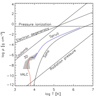
Figure 1.The boundaries in theT–ρplane at which different non-ideal effects start to be significant. The boundaries are estimated for the case of the pure hydrogen plasma (after Hansen et al., 2004). TheT–ρ dependency of the 1-D models of the solar atmosphere (VALC model, red curve) and of the solar convection zone (after Spruit (1974), blue) is indicated. The shaded area shows the portion of theT–ρ plane occupied by a typical snapshot from a 3-D HD simulation.
While both studies clearly indicate that the results of the different realistic simulations provide a consistent qualitative and quantitative description of the solar convection, the dif-ferences between different simulation runs are still present. Moreover, these differences may become significant in cer-tain experiments and measurements. A good example is the problem of the abundance measurement from the compari-son of the synthetic and observed spectra. This problem is extremely model-dependent, and high accuracy is critical.
In this paper we isolate the influence of the EOS on the hydrodynamical convection simulations. In Sect. 2, we quan-titatively compare an ideal and a nonideal equilibrium EOS. They represent the main two types of EOS used in the realis-tic simulations. A simple numerical experiment designed to study the propagation of the differences caused by different EOSs through the simulated domain and in time is described in Sect. 3.
2 Ideal versus nonideal EOS
Two types of EOS are used in the codes for the solar convec-tion simulaconvec-tions: (1) the nonideal EOS including the effects of the pressure ionisation, Coulomb interaction and electron degeneracy and (2) the ideal EOS for a mixture including the partial ionisation effects. MHD1(Hummer and Mihalas, 1988; Mihalas et al., 1988) and OPAL (Rogers et al., 1996; 1MHD here stands for the authors Mihalas, Hummer and Däp-pen (Mihalas et al., 1988).
Rogers and Nayfonov, 2002) are commonly used nonideal EOSs. The former is used in Stagger, the latter in MURaM, RHD, in the ANTARES code (Grimm-Strele et al., 2015) and in the MANCHA code (Khomenko et al., 2014). The ideal EOS of Wolf (1983) is implemented in Co5Bold. MU-RaM can work with a simple ideal EOS described in Vögler et al. (2005), while MANCHA incorporates an algorithm for the evaluation of the ideal EOS of a partially ionised mix-ture described by Vardya (1965) and improved by Mihalas (1967) and Wittmann (1974) (we shall refer to this EOS as VMW). The VMW algorithm is implemented in several ra-diative transfer codes to provide the electron pressure for known temperature and gas pressure (e.g. Bellot Rubio et al., 1999; Socas-Navarro, 2011).
The range of validity of the ideal EOS may be estimated for the trivial case of partially ionised pure hydrogen. In Fig. 1, we reproduce Fig. 3.9 of Hansen et al. (2004), show-ing theT–ρ plane with the boundaries for the nonideal ef-fects and the curve where the ionisation fraction of hydro-gen is 0.99. To Fig. 1 we add plots of two 1-D stratifications (the chromospheric VALC model of Vernazza et al. (1981) and the convection zone model of Spruit, 1974) and the area covered by a typical 3-D HD simulation (shaded area). All three models are within the limits of where the ideal EOS for pure hydrogen is valid. The deep end of the convection-zone model is close to the pressure–ionisation boundary, while, on the other end, the ionisation of hydrogen in the chromo-sphere requires a non-equilibrium solution of hydrogen ioni-sation (Carlsson and Stein, 2002) that cannot be represented by a simple curve in this plot. Nevertheless, the near-surface convection and the photosphere fall in the region of theT–ρ plane, where the ideal EOS is a safe assumption.
To compute nonideal EOS is extremely time-consuming and impossible to do on the fly in codes for 3-D numeri-cal simulations. Instead EOS is precomputed and results are stored in lookup tables suitable for fast interpolation. The computational cost of the ideal EOS is much lower; however, when the molecules are taken into account, it is necessary to solve the equations iteratively, and, therefore, the use of the precompiled lookup tables may save considerable computing time as long as the table grid is sufficiently fine to limit the interpolation errors.
2.1 Ideal EOS for partially ionised mixture
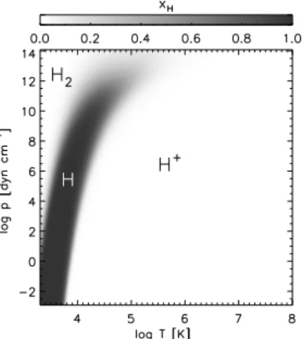
Figure 2.The ionisation fraction of hydrogen in theT–pgrid com-puted with the VMW EOS. Those portions of the domain that are dominated by the neutral H, H2molecule and H+are indicated.
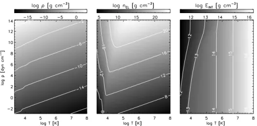
partition function data for H2and H+2 come from the survey of Sauval and Tatum (1984). The chemical equilibrium con-stants and the energies of the rotational–vibrational bound states are evaluated using these partition functions. Internal energy is defined up to an arbitrary constant. We follow the choice made in the OPAL and MHD EOS and set the poten-tial component of the internal energy to 0 when all hydro-gen atoms are in the ground state of the H2 molecule and all other atoms are neutral and in their atomic ground states. For the chemical composition we adopt the high-metallicity abundances of Anders and Grevesse (1989). Since our prime interest here is differential analysis, the choice of the abun-dance set is not critical. On the other hand, the set of Anders and Grevesse is built into the OPAL EOS and cannot be al-tered once the tables are produced. We do not compare the VMW directly to other ideal EOSs as they are based on the very similar approach and the differences among them are minor as long as the same chemical composition is selected. We evaluated the VMW EOS for a largeT–pgrid cover-ing 17 orders of magnitude in pressure and nearly 6 in tem-perature. This range of values matches the range of the OPAL EOS tables. Figure 2 shows the ionisation fraction of hydro-gen,xH=nH/nHtot, withnHandntotH being the number density of the neutral hydrogen and the total number density of the hydrogen atoms and molecules. Figure 3 shows the distribu-tion in the logT–logpplane of the mass density, the electron number density and the specific internal energy per mass2.
2.2 Nonideal EOS: OPAL
The OPAL EOS is computed in the physical picture through an activity expansion of the grand canonical partition func-tion of the plasma. The results are distributed as lookup
ta-2Hereafter we use “internal energy” for the specific internal en-ergy per mass.
bles3of the internal energy, the pressure, the electron density and other derived thermodynamical quantities as functions of the temperature and the density of several chemical com-positions. We reversely interpolate the tables (for the mass fractionX=0.7062 andZ=0.0197, corresponding to the
abundances of Anders and Grevesse) to obtain the internal energy, the density and the electron pressure in theT–p co-ordinates. The interpolation is performed using the method of the overlapping biquadratics that is included in the dis-tribution of the OPAL EOS. The results for the internal en-ergy and the density shown in the same range of the temper-ature and pressure as in Fig. 3 are visually nearly identical to the results of VMW. The electron density distribution shows a number of artefacts in the low-temperature region where ad hoc electron density is introduced (Rogers and Nayfonov, 2002), while it is similar to the VMW distribution elsewhere. Trampedach et al. (2006) examined the differences between the OPAL EOS and the MHD EOS.
2.3 Comparison
The relative differences between the mass density, the elec-tron number density and the internal energy in the VMW and the OPAL EOS in the logT–logp plane are shown in Fig. 4. The positive values indicate that the VMW quantity is larger. The largest differences in the density and the internal energy occur in the area with a temperature below 106K for pressure higher than 106dyn cm−2and densities higher than 10−6g cm−3. This is the area where hydrogen is still neutral in the VMW EOS (cf. Fig. 2). The OPAL tables do not in-clude the partial pressures of different particles needed for a direct comparison. However, the negative difference (the red area) in the density at constant pressure together with correspondingly higher internal energy and the electron den-sity indicate that the VMW hydrogen ionisation fraction is higher than the one from OPAL. The opposite applies for the blue area. While the latter may be interpreted as the ef-fect of the pressure ionisation (cf. Fig. 1), it is difficult to attribute the former to any particular effect without knowing the partial pressures consistent with the OPAL. Nevertheless, the area where the differences appear is not covered by the near-surface convection. At low pressure and a temperature below ≈2×10⁴K, the relative differences are below 1 %
(except for the electron densities at lowT, where the arte-facts dominate). Figure 5 shows a blow-up of Fig. 4 in that region. Vertical stripes in the density plot and the horizontal stripes in the electron pressure are due to the interpolation errors (coming from the reverse interpolation of the OPAL table to theT–ρdomain)4. The vertical bands below 3500 K in the relative difference of the electron density correspond
3http://opalopacity.llnl.gov/EOS_2005/
Figure 3.The mass density, the electron number density and the specific internal energy per mass computed on the temperature–pressure grid using the VMW EOS.
Figure 4.The relative difference between the VMW EOS and the OPAL EOS in the mass density, the electron number density and the internal energy ((VMW-OPAL)/VMW). The VMW EOS is computed on theT–pgrid and the OPAL EOS computed on theT–ρgrid and then interpolated to theT–pgrid. The two EOSs are computed for the same mass fractions. The contour lines are copied from Fig. 3 for comparison.
to the area where the OPAL electron densities are unreliable.
3 The convection simulation
To study propagation with time of differences caused by EOS choice in a near-surface convection simulation, we initiate and run two simulations with all parameters identical except for the EOS lookup tables. For this experiment we use the version of the MURaM code described in Vögler (2003) with several minor adaptations needed to run the code with an al-ternative set of EOS lookup tables. The code requires two tables, one with the temperature and the density tabulated as functions of the internal energy and the pressure and another with the temperature and the pressure as functions of the in-ternal energy and the density. The required tables are pro-duced from the VMW and the OPAL EOS described above. Since we are primarily interested in the relative difference
between the two runs and not in the physical realism of the result, we set up a simple HD convection run in 2-D with grey opacities. The physical size of the domain is 6.0 Mm in the horizontal direction and 1.4 Mm in the vertical, with 288 and 100 grid points respectively. The bottom boundary is open for the mass flow, the top boundary is closed and the vertical boundaries are set as periodic. The mass fluctuations through the bottom boundary are dynamically adjusted by the bound-ary pressure of the upflowing materialpup(see Vögler, 2003, Eq. 3.56, p. 32).
Figure 5.Blow-up of Fig. 4 in the low-pressure and low-temperature region relevant for the near-surface convection. The fragments of the contour lines from Fig. 4 are added.
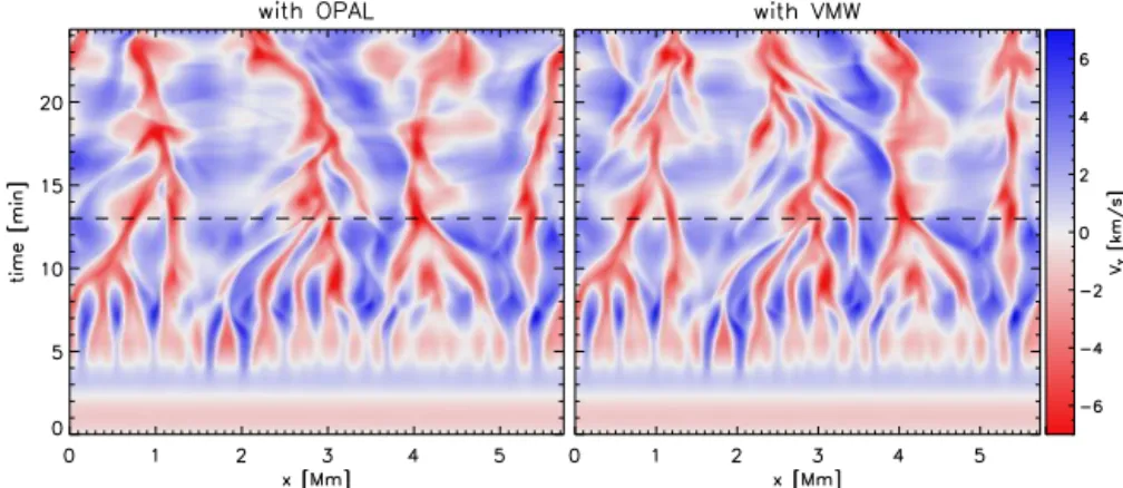
Figure 6.Vertical velocity at fixed height (850 km above the bottom of the simulation box) over the first 24 min of the simulation with the OPAL EOS (left) and with the VMW EOS (right). The dashed line approximately marks the instance when the two simulation runs separate.
The specific energy in the snapshots is then perturbed with a multiplicative factor of 1±0.05, with identical
randomisa-tion over the simularandomisa-tion box. We start the runs with a damp-ing factor for the radiative exchange term, gradually releas-ing it until the convection cells fully develop. Once the simu-lation is in the statistically steady state, we let it run for about 16 h of solar time while taking a snapshot every 20 s.
3.1 Results
In the first iteration step, the relative difference between the temperature in the two runs is within ±0.2%, which is in
agreement with Fig. 5. As the flows develop and accelerate in the initial phase, the differences between the runs grow and the point-by-point comparison between their parameters becomes meaningless. Figure 6 shows the velocity for the two runs at constant height in the box (850 km above the bot-tom of the box) versus time. The flows in the two cases are indistinguishably similar over the first 13 min; after that ini-tial phase they take different evolutionary paths toward the statistically steady solutions.
In MURaM the flux of the emergent radiationFoutis con-trolled by the specific energy of the upflowing material at the bottom boundary so that its mean value matches the value of the real sun (see Vögler, 2003, Eq. 3.50, p. 30). The relative difference of the meanFoutfor the two runs is thus small, as expected: 0.3 %. The temperature profiles of the two runs averaged over time and over the horizontal direction are very similar. The difference in the geometrical height scale (left panel) and in the scale of the continuum optical depth at 500 nm (right) is shown in Fig. 7. The largest absolute dif-ference between the two in the geometrical height scale is at 0.8 Mm above the bottom of the box and amounts to nearly 200 K (the relative difference is 2.3 %). This is the region where the radiative cooling begins to dominate producing a steep gradient of temperature with height. In the continuum optical depth scale at 500 nm, in the photosphere (τ500≤1),
Figure 7.The difference between the mean temperature of the simulation runs with OPAL and VMW in the geometrical height scale (left) and in the continuum optical depth scale at 500 nm (right). Note different scales in the two panels.
4 Conclusions
The tables of thermodynamical quantities (the mass density, the specific internal energy and the electron density) com-puted using two equations of state – one ideal (VMW, af-ter Vardya, 1965; Mihalas, 1967; Wittmann, 1974) and one nonideal (OPAL, Rogers et al., 1996; Rogers and Nayfonov, 2002) and both widely used in solar physics – are compared. The relative differences between the quantities in the region of the T–p plane usually considered in the realistic near-surface convection simulations (approximately 1 Mm below the level where the mean continuum optical depth is equal to 1 and 0.5 Mm above it) are below 1 %, except for the elec-tron density at the low temperatures, where the values of the OPAL tables are not reliable. Since we have access only to the tables precomputed with the OPAL code but not to the code itself, we cannot determine the origin of these differ-ences. Possible causes are the differences in the atomic and molecular data, in the approach and the interpolation errors.
To check how this difference may affect the result of the hydrodynamical simulations, we simulated the 2-D so-lar convection with the two EOSs with an otherwise identi-cal set-up. The two simulation runs separate in the parameter space as soon as the convective cells are developed. Never-theless, they evolve separately to a statistically nearly identi-cal steady state, with the temperature difference in the opti-cal depth sopti-cale below 10 K throughout the photosphere. This experiment demonstrates that the two EOSs are interchange-able for simulations of near-surface solar convection. More-over, the electron density in the OPAL tables, corrupted at low temperatures, may be recomputed for a large portion of theT–ρgrid of OPAL with an accuracy better than 1 % using the VMW ideal EOS (cf. Fig. 4). To estimate what the effect of the EOS choice in a more realistic set-up is (3-D, with magnetic field, non-grey radiative transfer including scatter-ing, etc.), it would be necessary to repeat this experiment in such conditions. The change of the mean temperature be-tween 2-D and 3-D solar convection simulations has been described by Asplund et al. (2000a) (see lower panel of their Fig. 9). Without analysing the origin of the differences in
their study, it may be noted that these differences are of the same order as the differences between the highly realistic 3-D H3-D simulations performed by different codes (Beeck et al., 2012). In any case, we do not expect significant changes in our results as long as the temperature and the density in a simulation remain within nearly the same range of theT–ρ plane as in our experiment.
This result is in agreement with the studies of Beeck et al. (2012) and Tanner et al. (2012), demonstrating robustness of the near-surface simulations. Regarding the deep convection, this result is consistent with the conclusions of Bahcall et al. (2004) that the depth of the convection zone does not depend significantly on the uncertainties in the EOS. It is also con-sistent with the recent study of Lord et al. (2014), who com-pared the effect of the OPAL EOS and a simple Saha-based EOS on the horizontal velocity spectrum of a solar deep con-vection simulation and found that the two produced nearly identical results, especially in the higher portion of the con-vection zone.
Acknowledgements. This work is partially supported by the Span-ish Ministry of Economy and Competitiveness (MINECO) through projects AYA2011-24808, AYA2010-18029 and AYA201455078-P. This work contributes to the deliverables identified in FP7 European Research Council grant agreement 277829, “Magnetic connectivity through the Solar Partially Ionized Atmosphere”. This research has made use of NASA’s Astrophysics Data System.
The topical editor L. Ofman thanks two anonymous referees for help in evaluating this paper.
References
Anders, E. and Grevesse, N.: Abundances of the elements – Mete-oritic and solar, Geochim. Cosmochim. Ac., 53, 197–214, 1989. Asplund, M., Ludwig, H.-G., Nordlund, Å., and Stein, R. F.: The ef-fects of numerical resolution on hydrodynamical surface convec-tion simulaconvec-tions and spectral line formaconvec-tion, Astron. Astrophys., 359, 669–681, 2000a.
Bahcall, J. N., Serenelli, A. M., and Pinsonneault, M.: How Ac-curately Can We Calculate the Depth of the Solar Convective Zone?, Astrophys. J., 614, 464–471, 2004.
Beeck, B., Collet, R., Steffen, M., Asplund, M., Cameron, R. H., Freytag, B., Hayek, W., Ludwig, H.-G., and Schüssler, M.: Sim-ulations of the solar near-surface layers with the CO5BOLD, MURaM, and Stagger codes, Astron. Astrophys., 539, A121, doi:10.1051/0004-6361/201118252, 2012.
Bellot Rubio, L. R., Ruiz Cobo, B., and Collados, M.: An LTE code for the inversion of Stokes spectra from solar magnetic elements, in: Polarization, edited by: Nagendra, K. N. and Stenflo, J. O., Astrophys. Space Sc. L., 243, 271–280, 1999.
Carlsson, M. and Stein, R. F.: Dynamic Hydrogen Ionization, As-trophys. J., 572, 626–635, 2002.
Danilovic, S., Gandorfer, A., Lagg, A., Schüssler, M., Solanki, S. K., Vögler, A., Katsukawa, Y., and Tsuneta, S.: The intensity contrast of solar granulation: comparing Hinode SP results with MHD simulations, Astron. Astrophys., 484, L17–L20, 2008. Galsgaard, K. and Nordlund, Å.: Heating and activity of the solar
corona 1. Boundary shearing of an initially homogeneous mag-netic field, J. Geophys. Res., 101, 13445–13460, 1996.
Grimm-Strele, H., Kupka, F., Löw-Baselli, B., Mundprecht, E., Zaussinger, F., and Schiansky, P.: Realistic Simulations of Stel-lar Surface Convection with ANTARES: I. Boundary Con-ditions and Model Relaxation, ArXiv e-prints, 34, 278–293, doi:10.1016/j.newast.2013.11.005, 2015.
Hansen, C. J., Kawaler, S. D., and Trimble, V.: Stellar interiors: physical principles, structure, and evolution, Springer-Verlag, Ney York, USA, 2004.
Hummer, D. G. and Mihalas, D.: The equation of state for stellar en-velopes. I – an occupation probability formalism for the trunca-tion of internal partitrunca-tion functrunca-tions, Astrophys. J., 331, 794–814, 1988.
Irwin, A. W.: Polynomial partition function approximations of 344 atomic and molecular species, Astrophys. J. Suppl., 45, 621–633, 1981.
Khomenko, E. V., Martínez González, M. J., Collados, M., Vögler, A., Solanki, S. K., Ruiz Cobo, B., and Beck, C.: Magnetic flux in the internetwork quiet Sun, Astron. Astrophys., 436, L27–L30, 2005.
Khomenko, E., Díaz, A., de Vicente, A., Collados, M., and Luna, M.: Rayleigh-Taylor instability in prominences from numerical simulations including partial ionization effects, Astron. Astro-phys., 565, A45, doi:10.1051/0004-6361/201322918, 2014. Lord, J. W., Cameron, R. H., Rast, M. P., Rempel, M., and Roudier,
T.: The Role of Subsurface Flows in Solar Surface Convec-tion: Modeling the Spectrum of Supergranular and Larger Scale Flows, Astrophys. J., 793, 24, 2014.
Mihalas, D.: The Calculation of Model Stellar Atmospheres, in: Methods in Computational Physics, edited by: Alder, B. and Fernbach, S. R., vol. 7, Academic, New York, USA, 1967. Mihalas, D., Däppen, W., and Hummer, D. G.: The equation of state
for stellar envelopes. II – Algorithm and selected results, Astro-phys. J., 331, 815–825, 1988.
Nordlund, Å.: Numerical simulations of the solar granulation. I – Basic equations and methods, Astron. Astrophys., 107, 1–10, 1982.
Pereira, T. M. D., Asplund, M., Collet, R., Thaler, I., Trampedach, R., and Leenaarts, J.: How realistic are solar model
atmo-spheres?, Astron. Astrophys., 554, A118, doi:10.1051/0004-6361/201321227, 2013.
Rogers, F. J. and Nayfonov, A.: Updated and Expanded OPAL Equation-of-State Tables: Implications for Helioseismology, As-trophys. J., 576, 1064–1074, 2002.
Rogers, F. J., Swenson, F. J., and Iglesias, C. A.: OPAL Equation-of-State Tables for Astrophysical Applications, Astrophys. J., 456, 902–908, 1996.
Sauval, A. J. and Tatum, J. B.: A set of partition functions and equi-librium constants for 300 diatomic molecules of astrophysical interest, Astrophys. J. Suppl., 56, 193–209, 1984.
Shelyag, S., Schüssler, M., Solanki, S. K., and Vögler, A.: Stokes diagnostics of simulated solar magneto-convection, Astron. As-trophys., 469, 731–747, 2007.
Socas-Navarro, H.: A high-resolution three-dimensional model of the solar photosphere derived from Hinode observations, As-tron. Astrophys., 529, A37, doi:10.1051/0004-6361/201015805 . 2011.
Spruit, H. C.: A model of the solar convection zone, Sol. Phys., 34, 277–290, 1974.
Stein, R. F. and Nordlund, Å.: Simulations of Solar Granulation. I. General Properties, Astrophys. J., 499, 914–933, 1998.
Stein, R. F. and Nordlund, Å.: Realistic Solar Convection Simula-tions, Sol. Phys., 192, 91–108, 2000.
Tanner, J. D., Basu, S., and Demarque, P.: Comparing the Effect of Radiative Transfer Schemes on Convection Simulations, Astro-phys. J., 759, 120, 2012.
Tanner, J. D., Basu, S., and Demarque, P.: Variation of Stellar Enve-lope Convection and Overshoot with Metallicity, Astrophys. J., 767, 78, 2013.
Trampedach, R., Däppen, W., and Baturin, V. A.: A Synoptic Com-parison of the Mihalas-Hummer-Däppen and OPAL Equations of State, Astrophys. J., 646, 560–578, 2006.
Vardya, M. S.: Thermodynamics of a solar composition gaseous mixture, Mon. Not. R. Astron. Soc., 129, 205–213, 1965. Vernazza, J. E., Avrett, E. H., and Loeser, R.: Structure of the solar
chromosphere. III – Models of the EUV brightness components of the quiet-sun, Astrophys. J. Suppl., 45, 635–725, 1981. Vögler, A.: Three-dimensional simulations of magneto-convection
in the solar photosphere, PhD Thesis, Goettingen, http://www. solar-system-school.de/alumni/voegler.pdf, 2003.
Vögler, A., Shelyag, S., Schüssler, M., Cattaneo, F., Emonet, T., and Linde, T.: Simulations of magneto-convection in the solar photo-sphere. Equations, methods, and results of the MURaM code, Astron. Astrophys., 429, 335–351, 2005.
Wedemeyer, S., Freytag, B., Steffen, M., Ludwig, H.-G., and Hol-weger, H.: Numerical simulation of the three-dimensional struc-ture and dynamics of the non-magnetic solar chromosphere, As-tron. Astrophys., 414, 1121–1137, 2004.
Wedemeyer-Böhm, S. and Rouppe van der Voort, L.: On the con-tinuum intensity distribution of the solar photosphere, Astron. Astrophys., 503, 225–239, 2009.
Wittmann, A.: Computation and Observation of Zeeman Multiplet Polarization in Fraunhofer Lines. II: Computation of Stokes Pa-rameter Profiles, Sol. Phys., 35, 11–29, 1974.