Velocity of Front Propagation in 1-Dimensional
Autocatalytic Reactions
C. Warren[
z], E. Somfai[*], and L.M. Sander[
y]
Dept. ofPhysics,TheUniversityofMichigan,AnnArbor,MI48109-1120,USA
Received 1 December 1999
We study a discrete model of the irreversible autocatalytic reaction A+B !2A in one
dimen-sion. Looking at the dynamics of propagation, we nd that in the low-concentration limit the average velocity of propagation approachesv= =2, where is the concentration, and, in the high
concentration limit, we nd the velocity approachesv= 1,e , =2.
I Introduction
In this paper we study a discrete model of the irre-versible autocatalytic reactionA+B !2A in one di-mension. We analyze the velocity of reaction propaga-tion as a funcpropaga-tion of the total concentrapropaga-tion,. This re-action is a simple example of a chemical rere-action model, but we can also think of it as a representation of the spread of an infection. The A particles are infected, and we allow them to diuse, i.e. perform a random walk, and when a `sick' particle encounters a `healthy' one (a B particle) then the B is instantly infected. We assume that the A's and the B's see each other only by infection. Otherwise they are independent random walkers which do not interact. The quantity of interest is the speed of the spread of the infection. If we start with one A on the extreme left of the system, we are asking for the time dependence of the location of the rightmost A.
Models of this type have evoked a good deal of in-terest [1-4] because of several unexpected, fascinating features of the process. As we will see, in the limit of small the front propogation is dominated by uctu-ation eects. What attracted particular attention [1] was the realization that, as a result, continuum model-ing breaks down completely for this reaction.
Specically, we expect that the mean concentra-tion of A particles would be described by the Fisher-Kolmogorov equation [5], as we can see by writing a conventional reaction-diusion equation:
@ t
a = D @ xx
a+k ab = D @
xx
a+k a(,a) (1) Here k is a rate constant, D the diusion constant, and we have used the fact that a +b = . The last equation becomes the Fisher-Kolmogorov equation @
t u=@
xx
u+u(1,u) after changing variables. Now
from the standard theory [6], the velocity of the front approachesv
c = 2 p
k D independent of initial condi-tions.
However, simulations [1] showed that the front ve-locity waslinearin for small , and thus very much smaller than expected. This is understandable from the work of Brunet and Derrida [2] who pointed out that discreteness has an anomalously large eect on systems which obey the Fisher-Kolmogorov equation in the continuum limit. In references [2, 3] models were introduced which interpolated between the results of [1] and the Fisher-Kolmogorov equation via a very slow crossover. The models involved a very large density of particles with a small reaction rate. They found that the velocity depression was given byvv
c
,K =ln 2
() whereK is a constant.
A question remains, however: What is the mecha-nism for the small velocity for ! 0 in the original A+B ! 2A process? In a trivial model of indepen-dent random walkers, it is startling that there is any interesting dynamics. The total density at any point is clearly given by a Poisson distribution. It turns out however, that the front is not a typical point, and this is the key to the unexpected behavior.
We nd that the small velocity is a giant uctuation eect which goes qualitatively as follows. Suppose we assume that the velocity is a monotonically increasing function of, and, for smallrecall that there are large uctuations in the local density. The front will move quickly through high density regions, and get stuck in the low density ones. Thus, on average, the motion will be dominated by congurations where the front is behind a gap in the distribution of B's. The front mo-tion will be random, and not advance, as long as the rightmost A cannot convert a B. Our simulations and analysis in the next section support this picture.
right we consider the case of large for a parallel up-dating version of the process. Clearly the velocity must approach one lattice constant per unit time since there will always be a conversion at each step. However, the nature of this approach turns out to be tricky, and we are able to give only a partial analysis.
II Model and simulation results
Consider a 1-D lattice of length L [7] populated with random walkers randomly distributed with concentra-tion . The leftmost particle is of type A, and all of the other particles are of type B. The particles make random steps with parallel updating, i.e., all the parti-cles move simultaneously. Any number of partiparti-cles are allowed to occupy a site. If a B particle encounters or passes an A particle, it becomes an A particle. The rightmost A particle denes the propagation front, and we are interested in the velocity of this front.
Figure 1. Mean number of particles for sites about the front from a simulation with an average of 0.2 particles/site (in the rest frame of the front).
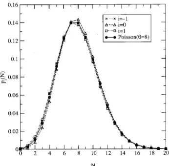
As we pointed out above, the particles follow a simple random walk and thus are Poisson distributed. However, taking into account particle types and follow-ing the front, the distribution of particles at the front or near the front is not so distributed. Fig. (1) shows the average density of particles from simulation for various sites around the front for = 0:2. Ignoring the t for the moment, the density (conditioned on there being a front at i = 0), is depleted to the right of the front. At higher concentrations, Fig. (2) shows the probabil-ity distribution of particles at various sites around the front in a simulation with average concentration= 2; Fig. (3) is for= 4, and Fig. (4) for= 8.
Figure 2. Probability density of site i about the front from a simulation with an average of 2 particles/site (in the rest frame of the front).
Figure 3. Probability density of site i about the front from a simulation with an average of 4 particles/site.
Our simulations were performed in two dierent ways. For concentrations below = 0:5, 200 walkers were simulated and lengths were adjusted accordingly, L= 200=. Enough time steps were performed for each walker to walk on average halfway across the sample, T =L=. To avoid initial transients calculations were also made with the rst 40=
Figure 4. Probability density of site i about the front from a simulation with an average of 8 particles/site.
An earlier study [1] analyzed the velocity in an ap-proximate fashion, using the Smoluchowski approach. In this method, centered in the rest frame of the front, B particles diuse toward the front. The number den-sity n follows the one-dimensional diusion equation in the frame moving with velocity v,
@n @t
,v n 0=
n 00
; (2)
where the diusion constantD = 1. Assuming station-arity, the time derivative vanishes, and the boundary conditions n(1) = , n
0(
1) = 0 and n(0 +) = 0 lead to:
n(x) = ifx<0 = (1,exp
,v x)
ifx0: (3) We will see later that v / so that, as x! 0
+, nis order
2. As shown by Fig. 1, this distribution agrees well with simulation. However, the analysis gives no way to nd v.
II.1 Small
In the low-concentration limit, 1, consider a region containing the front particle and the \second" particle, i.e., that nearest the front. (In case of more than one particle ati= 0 we arbitrarily declare one to be the front, and the other the second particle.) The size of the region will be 1=. Dene a coordinate system in the rest frame of the front particle, whose position is dened to be at i = 0. The number den-sity of the second particle at site i at time t is n
i( t). Note that since the front particle is treated separately and not included inn
i, the latter approaches the prob-ability distribution for the second particle in the limit !0.
The location of the second particle is the key to cal-culating the velocity. In fact, the only nonzero contri-butions to the average velocity occur when the second particle is one behind the front (i=,1) or on the front (i = 0). For all other positions, the front particle un-dergoes an unbiased random walk, and the front does not move on average. When i =,1, with proper re-naming of particles, the front will move forward one step with probability 1/2, stay the same with probabil-ity 1/4 and move back one with probabilprobabil-ity 1/4. Thus, giveni=,1, the average velocity is 1=2,1=4 = 1=4. Wheni= 0, the front will move forward one with prob-ability 3/4 and move back one with probprob-ability 1/4, so the average velocity of the front is
v(t) = 14n ,1(
t) + 12n 0(
t): (4)
From random walk dynamics, the motion of the sec-ond particle obeys a few simple rules:
If the particle is at i= 0 at timet,n ,2(
t+ 1) = 1=2 andn
0(
t+ 1) = 1=2.
If the particle is ati=,1 at timet,n ,1(
t+1) = 3=4 andn
,3(
t+ 1) = 1=4.
Otherwise, if the particle is at i < ,1 or i > 0, n
i+2(
t+1) = 1=4,n i(
t+1) = 1=2 andn i,2(
t+1) = 1=4. (Note that in these expressions the position of the sec-ond particle is dened with respect to the front at at timet+ 1.)
For a stationary distribution,n i(
t) =n i(
t+1)n i, so the rules lead to relationships between the densities: (a) For positions away from the front,i<,2 ori>2,
n i= (
n i,2+
n i+2)
=2: (5)
(b) For positions around the front
n ,2 =
n ,4
=2 +n 0 n
,1 = n
,3+ n
1 n
0 = (
n ,2+
n 2)
=2 n
1 =
n 3
=2 n
2 =
n 4
=2 (6)
Equation (5) implies a linear behavior for the proba-bilities away from the front. We need to impose bound-ary conditions far from the front, because we have made the approximation of only one nonfront particle, which is only valid in the region 1=around the front. We do this by matching to the continuum solution of Eq. (3). For (3) to order , the density is simply behind the front and 0 in front of the front. Thus, to rst order in concentration, the solution to the equations above is:
n i=
8 < :
ifi<0 =2 ifi= 0 0 ifi>0
: (7)
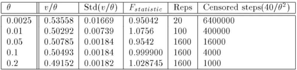
v = Std(v =) F
statistic Reps Censored steps(40 =
2) 0.0025 0.53558 0.01669 0.95042 20 6400000
0.01 0.50292 0.00739 1.0756 100 400000
0.05 0.50785 0.00184 0.9542 1600 16000
0.1 0.50493 0.00184 0.999900 1600 4000 0.2 0.49152 0.00182 1.028745 1600 1000
Table 1. Simulation results for the velocity of front propagation for low concentrations.
Note that including the front particle, to rst order, the stable totalnumber density distribution isN
i = fori<0,N
i = 1 +
=2 fori= 0, andN
i= 0 for i>0. That is we have average concentration to the left of the front and a depleted zone to the right, in agreement with simulations.
Note the bipartite nature of (5) -(6). We can con-sider a simpler \even-lattice" model in which only the even sites are populated and still get the same average velocity. This avoids the complicating factor of a site -1 particle passing the front particle and becoming the new front particle. For the even sites,
n
i = ( n
i,2+ n
i+2)
=2; i<,2 or i>2 n
,2 = n
,4 =2 +n
0 n
0 = (
n ,2+ n 2) =2 n 2 = n 4
=2 (8)
Maintaining the same overall density would mean doubling the concentration at all of the sites. Look-ing at the form of (4) and takLook-ing into account dierLook-ing number densities, we get equal contributions to the ve-locity from site 0 and site -1, and thus the same low velocity limit,v= =2. However, this simplied \even-lattice" model does not approach the same limit as that of the \full-lattice" model in high concentration.
II.2 Large
In the full-lattice model, for any concentration the probability of the front moving backward one site is
P ,= 1 X n 0 =1 1 X n ,1 =0 1 2n 0 +n ,1 p(n
0 ;n
,1)
; (9)
moving forward one is
P += 1 X n0=1 1, 1 2n0 p(n
0) (10)
and being stationary is
P 0= 1 X n 0 =1 1 X n ,1 =0 1 2n0 1, 1 2n,1 p(n
0 ;n
,1)
; (11) where p(n
i) is the probability of site
i havingn i parti-cles.
With stationarity, p(n 1(
t);:::;n L(
t))
p(n 1
;:::;n
L), we can use the dynamics of the model to obtain similar relations between the site averages and other site moments. In the rest frame of the front, if the front moves forward, site i at time t is \fed" by sitesiandi+2 at timet,1. If the front is stationary, site iis fed by sitesi,1 andi+ 1. If the front moves backward, site i is fed byi and i,2. The average at site iis
c hn
i i=P
+ hf
i+ b
i+2
j+i+P 0
hf i,1+
b i+1
j0i+P , hf i+ b i,2 j,i; (12) d wheref
k is the number of particles that move forward from site k, b
k is the number of particles that move backward from site k, n
k = b
k+ f
k,
hj+imeans that the average is conditioned on the front moving forward,
hj0imeans the average is conditioned on the front re-maining stationary andhj,imeans the average is con-ditioned on the front moving backward.
For example, for sitei= 0, c
hn 0
i=P +
hf 0+
b 2
j+i+P 0
hf ,1+
b 1
Note that around the front, specically for i 2 f,2;,1;0;1;2g, the movement of the front reveals in-formation about the number particles at sitei.
Now consider to be large. Assume for the mo-ment that the distribution at all sites, includingi= 0, is Poisson with mean
i, as seen in the simulations. Al-though this must be true far from the front, it is not clear why it is true nearby. It introduces a discrepancy
of ordere
, because at site
i= 0 there is a probability e
, that there will be no particles at site
i= 0. This cannot be true because i = 0 is dened as the site of the rightmost A particle.
Neglecting this inconsistency for the moment, for large, one may use equation (13) to derive a recursion relation:
c
0= (1 ,e , 0 2 ) 2 2 + 0 2 +e
, 0 2(1 ,e , ,1 2 ) 1 2 +e
, 0 2 ,1 2 +e
, 0 + ,1 2 ( 0+ ,2
2 ): (14)
With the assumption i
, this equation collapses to a relation that approaches self-consistency to order 1 2 e , 2. A similar relation may be derived for the variance of the number of particles at sitei,
hn 2 0
i,hn 0
i 2=
P +
h(f 0+
b 2)
2
j+i+P 0
h(f ,1+
b 1)
2 j0i+P
, h(f
0+ b
2) 2
j,i,hf 0+ b 2 i 2 : (15) d With the Poisson assumption of mean and variance , this relation simplies to an expression that is self-consistent to leading order 5
4 2 e , 2.
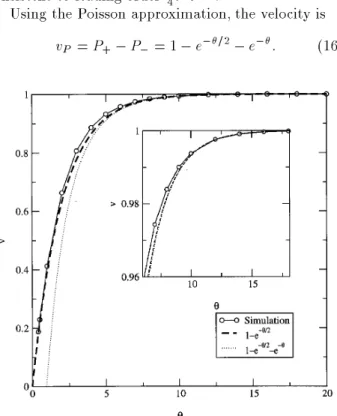
Using the Poisson approximation, the velocity is
v P =
P +
,P ,= 1
,e , =2
,e ,
: (16)
Figure5. Meanfrontvelo city asafunctionofparticle con-centration.
However we can handlep(n
0= 0) in a dierent way by using a conditioned or truncated Poisson distribu-tion, p
T [8]. Specically, p(n
0= 0) = e
, is truncated from the distribution and distributed to the other prob-abilities,
p T(
n 0=
k) =
0 ifk= 0
(1,e ,),1
p P(
k) ifk6= 0
: (17)
wherep P(
k) is the ordinary Poisson distribution. Then the velocity is
v T = 1
,e , =2
: (18)
The recursion relation discrepancy for the mean is iden-tical to that of the Poisson distribution since everything is simply divided by 1,e
,, and the leading order of the variance is again identical, 5
4 2 e ,
2. Fig. (5) shows that this agrees with the data better than Eq. (16). We have no explanation for this.
III Summary
We have seen that the behavior ofv at low concentra-tion can be traced to the depleconcentra-tion zone to the right of the front. Near the front the distribution of particles is very dierent from the Poisson distribution, and the motion of the front is dominated by the depletion. For large the velocity is approximated by 1,e
, =2 and the distribution is quite close to the truncated Poisson. In the low concentration limit, to order, the veloc-ity is simplyv = =2 in the truncated Poisson model, which also is correct. However, the truncated Poisson model does not satisfy the recursion relations to order and it lacks the depletion zone ahead of the front. As shown in Fig. (5), the truncated Poisson approach gives a reasonable approximationforvfor any concentration, but this should be regarded as only a convenient inter-polation.
References
[z] email: [email protected]
[*] Current address: Instituut Lorentz, Leiden, NL-2333 CA, Netherlands. email [email protected] [y] email: [email protected]
[1] J. Mai, I.M. Sokolov, and A. Blumen, Phys. Rev. Lett.
77, 4462 (1996)
[2] E. Brunet and B. Derrida, Phys. Rev. E 56, 2597
(1997).
[3] D. A. Kessler, Z. Ner and L. M. Sander, Phys. Rev. E
58, 107 (1998).
[4] J. Riordan, C. Doering, and D.ben-Avraham Phys. Rev. Lett.75, 565 (1995).
[5] R. A. Fisher, Annals of Eugenics 7, 355 (1937); A.
Kolmogorov, I. Petrovsky, and N. Piscounov, Moscow Univ. Bull. Math. A1, 1 (1937).
[6] J. D. Murray,Mathematical Biology(Springer, Berlin, 1993).
[7] To simulate the dynamics of a large lattice, we actually used a ring lattice of L sites to handle the far bound-aries, left and right. Random A walkers that walked o the left edge were added to the right edge as B walkers, and vice versa.