www.atmos-meas-tech.net/6/895/2013/ doi:10.5194/amt-6-895-2013
© Author(s) 2013. CC Attribution 3.0 License.
Atmospheric
Measurement
Techniques
Geoscientiic
Geoscientiic
Geoscientiic
Geoscientiic
Global tropospheric ozone column retrievals from OMI data by
means of neural networks
A. Di Noia1,2,*, P. Sellitto3, F. Del Frate1, and J. de Laat2
1Earth Observation Laboratory, Department of Civil and Computer Engineering, Tor Vergata University, via del Politecnico 1,
00133 Rome, Italy
2Royal Netherlands Meteorological Institute (KNMI), Wilhelminalaan 10, 3732 GK De Bilt, the Netherlands
3Laboratoire Inter-universitaire des Systèmes Atmosphériques (LISA), UMR7583, Universités Paris-Est et Paris Diderot,
CNRS, Rue du Général de Gaulle, 94010 Créteil, France
*now at: SRON Netherlands Institute for Space Research, Sorbonnelaan 2, 3584 CA Utrecht, the Netherlands
Correspondence to:A. Di Noia ([email protected])
Received: 2 October 2012 – Published in Atmos. Meas. Tech. Discuss.: 22 October 2012 Revised: 5 February 2013 – Accepted: 13 March 2013 – Published: 9 April 2013
Abstract. In this paper, a new neural network (NN) algo-rithm to retrieve the tropospheric ozone column from Ozone Monitoring Instrument (OMI) Level 1b data is presented. Such an algorithm further develops previous studies in order to improve the following: (i) the geographical coverage of the NN, by extending its training set to ozonesonde data from midlatitudes, tropics and poles; (ii) the definition of the out-put product, by using tropopause pressure information from reanalysis data; and (iii) the retrieval accuracy, by using an-cillary data (NCEP tropopause pressure and temperature pro-file, monthly mean tropospheric ozone column from a satel-lite climatology) to better constrain the tropospheric ozone retrievals from OMI radiances. The results indicate that the algorithm is able to retrieve the tropospheric ozone column with a root mean square error (RMSE) of about 5–6 DU in all the latitude bands. The design of the new NN algorithm is extensively discussed, validation results against independent ozone soundings and chemistry/transport model (CTM) sim-ulations are shown, and other characteristics of the algorithm – i.e., its capability to detect non-climatological tropospheric ozone situations and its sensitivity to the tropopause pressure – are discussed.
1 Introduction
Ozone is one of the most important trace gases in the Earth’s atmosphere. Ozone is most abundant in the stratosphere, where it shields the troposphere from harmful ultraviolet ra-diation. In the troposphere, ozone acts as a precursor of the hydroxyl (OH) radical, which is able to remove pollutants from the troposphere via oxidation reactions (Jacob, 1999). Furthermore, tropospheric ozone is a pollutant itself, since it is harmful for the biosphere when it reaches high concentra-tions near the Earth’s surface (Heck et al., 1982; Lippmann, 1989). Finally, tropospheric ozone acts as a greenhouse gas (Shindell et al., 2006).
Tropospheric ozone variations may occur over relatively small spatial scales. Concentrations of tropospheric ozone are affected by several factors. First, they depend on the concentrations of its precursors – namely, nitrogen oxides (NOx), carbon monoxide (CO) and volatile organic
com-pounds (VOCs) – which are either emitted as a consequence of human activities or due to natural causes (e.g., light-ning, which produces NOx). Since tropospheric ozone is
at midlatitudes (see, e.g., Shapiro, 1980). Long-range trans-port of tropospheric ozone and its precursors also affects its spatial distribution (Carmichael et al., 1998; Creilson et al., 2003).
Monitoring tropospheric ozone using satellite instruments is important in order to obtain a global picture of its distri-bution. However, several difficulties are encountered in in-ferring tropospheric ozone concentrations from satellite ob-servations. First, the contribution of tropospheric ozone to the measured radiances is much weaker than the contribution coming from stratospheric ozone. Second, current ultravio-let or thermal infrared measurements have usually a reduced sensitivity to lower tropospheric ozone (Natraj et al., 2011, and references therein).
The first attempts to derive information on tropospheric ozone from satellite observations date back to the 1980s. Fishman et al. (1986, 1987) first suggested that total ozone measurements made from the Total Ozone Mapping Spec-trometer (TOMS) could contain information on cases of en-hanced tropospheric ozone. In the first algorithms for quan-titative tropospheric ozone retrievals, the information on tro-pospheric ozone was obtained by subtracting a stratospheric ozone column measurement from a colocated total ozone measurement. The stratospheric ozone column was estimated from limb observations (Fishman and Larsen, 1987; Fish-man, 2000, and references therein) or from ozone column measurements above high convective clouds (Ziemke et al., 1998, 2001; Ahn et al., 2003; Newchurch et al., 2003) or high mountains (Jiang and Yung, 1996; Kim and Newchurch, 1996; Newchurch et al., 2001). An alternative approach, specifically designed for TOMS observations, was to directly infer tropospheric ozone information based on the depen-dence of TOMS total ozone columns on the scan angle of the instrument (Kim et al., 1996, 2001, 2004).
More recently, after the development of new satellite in-struments, with hyperspectral measurement capabilities, the direct determination of tropospheric ozone from the UV/VIS part of the spectrum has become feasible (Munro et al., 1998; Liu et al., 2005, 2006, 2010). Nevertheless, residual tech-niques similar to those described above for TOMS have been also applied to hyperspectral data. For instance, Valks et al. (2003) developed a cloud-slicing algorithm for the Global Ozone Monitoring Experiment (GOME), whereas nadir-limb residual techniques have been used by Ziemke et al. (2006), Schoeberl et al. (2007), and Yang et al. (2007) to estimate tropospheric ozone column by subtracting Microwave Limb Sounder (MLS) limb stratospheric ozone columns from Ozone Monitoring Instrument (OMI) total ozone columns.
Another possibility to directly retrieve tropospheric ozone from satellite hyperspectral observations is the applica-tion of neural networks (NNs). NN algorithms for tropo-spheric ozone retrievals from OMI and the Scanning Imag-ing Absorption Spectrometer for Atmospheric Chartography (SCIAMACHY) have been recently developed (Sellitto et al., 2011, 2012, respectively). In particular, Sellitto et al. (2011)
developed an algorithm to retrieve tropospheric ozone from OMI data at northern midlatitudes, named the OMI-TOC NN. The algorithm yields daily estimates of the tropospheric ozone column from the surface to 200 hPa at the northern midlatitudes by using OMI reflectance spectra, solar zenith angle (SZA) at 19 wavelengths, and the total ozone column from the OMI-TOMS total ozone (OMTO3) Level 2 prod-uct (Bhartia and Wellemeyer, 2002). The performances of the OMI-TOC NN algorithm were shown to be compara-ble with those of the physics-based algorithms of Schoe-berl et al. (2007) and Liu et al. (2010) by means of a vali-dation exercise with ozonesonde measurements at northern midlatitudes, with root mean square (RMS) errors around 8 DU and correlation coefficients around 0.60 between the actual and the retrieved tropospheric ozone columns (Sellitto et al., 2011). Di Noia et al. (2013) further validated the OMI-TOC NN over a number of European ozonesonde stations, finding similar results, and pointing out the possible pres-ence of a negative bias in the OMI-TOC NN in cases of low tropopauses (tropopause pressures larger than approximately 250 hPa).
The main limitations of the OMI-TOC NN algorithm are its coverage, which is limited at the northern midlatitudes, and the choice to use the 200 hPa level as the upper inte-gration limit for the retrieved ozone columns, regardless of the actual tropopause conditions. In particular, this latter fea-ture raises the question of whether it is legitimate to say that the retrieved ozone columns are “tropospheric” since even at midlatitudes the actual tropopause pressure can be very dif-ferent from 200 hPa (Hoinka, 1998). In order to overcome this problem, a preprocessed tropopause height can be used as upper integration limit for the retrieved ozone columns. By doing so, it is possible to produce estimates that represent the actual “tropospheric” ozone column more realistically. For this study the thermal tropopause given by the National Center for Environmental Prediction (NCEP)/National Cen-ter for Atmospheric Research (NCAR) Reanalysis (Kalnay et al., 1996) has been used.
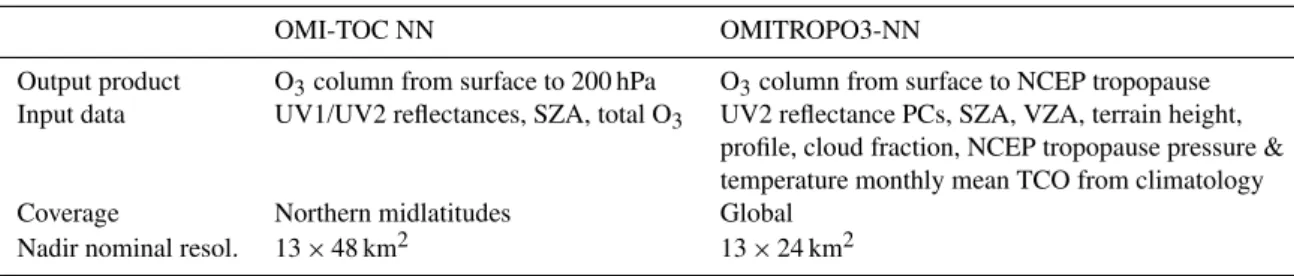
Table 1.Differences between the OMITROPO3-NN and the OMI-TOC NN algorithms. The OMI UV1 channel covers the range 270–310 nm, the OMI UV2 channel covers the range 310–345 nm. Acronyms: SZA (solar zenith angle), VZA (viewing zenith angle), PC (principal component), TCO (tropospheric column ozone).
OMI-TOC NN OMITROPO3-NN
Output product O3column from surface to 200 hPa O3column from surface to NCEP tropopause
Input data UV1/UV2 reflectances, SZA, total O3 UV2 reflectance PCs, SZA, VZA, terrain height,
profile, cloud fraction, NCEP tropopause pressure & temperature monthly mean TCO from climatology
Coverage Northern midlatitudes Global
Nadir nominal resol. 13×48 km2 13×24 km2
Besides these three key points, a number of additional technical issues are addressed in the preprocessing of OMI radiance and irradiance spectra (namely, several refinements were introduced in the data quality control and filtering rou-tines). Furthermore a different input dimensionality reduc-tion strategy is adopted, with a simple linear principal com-ponent analysis (PCA) used instead of the extended prun-ing (EP) technique. The new algorithm will be henceforth referred to as OMITROPO3-NN.
The paper is organized as follows. In Sect. 2 a general de-scription of NNs is given, with a particular focus on their use in the context of inverse problems; in Sect. 3 the gen-eration of the OMITROPO3-NN dataset is described and all the preprocessing steps are discussed; in Sect. 4 the choices made in the NN training are explained; general validation results are shown in Sect. 5; in Sect. 6 global tropospheric ozone fields retrieved on two dates during August 2006 are used as examples in order to give further insight into some of the characteristics of the OMITROPO3-NN; Sect. 7 presents conclusions and hypotheses for future work.
2 Neural networks in satellite retrievals
2.1 Basic concepts and terminology
NNs can be considered as algorithms for nonlinear regres-sion and function approximation. Although several types of NNs can be devised, they share a number of common charac-teristics: (i) the computation is distributed among elementary units (called neurons), and (ii) the relationship to be approx-imated is learned by the NN from a training dataset.
Mathematically, it can be said that an NN can be used to approximate an unknown relationship between two quanti-tiesx∈Rnandy∈Rmthrough a nonlinear model8Wsuch that
y=8W(x), (1)
whereWis a set of free parameters to be adjusted from a training dataset. In the case of supervised training, which is the only relevant case for the purposes of this work, the training dataset is made of pairs(xi,yi)of instances of the
relationship to be approximated. The adjustment of the free parameters is made according to a learning algorithm, which basically consists of an iterative minimization of an error cost function of the kind
C=f (kyi−8W(xi)k), (2)
with respect toW. According to the exact definition of the cost function and to the choice of the iterative method cho-sen for its minimization, several learning algorithms can be defined. The reader can refer to Bishop (1995) or Haykin (1999) for more detailed information.
2.2 Multilayer perceptrons
The multilayer perceptron (MLP) network (Werbos, 1974) is one of the most widespread NN architectures. Each neuron of an MLP realizes the input–output relationship
y=ϕ(wTx+b), (3)
wherewandbare the weight vector and the bias of the neu-ron, respectively, and are its free parameters to be adjusted, and the functionϕ, chosen in advance, is the activation func-tion of the neuron.
The neurons of an MLP are organized in layers: (i) an input layer, which simply contains the input vector of the MLP; (ii) at least one hidden layer, containing neurons with nonlinear activation functions; and (iii) an output layer, whose neurons can either have linear or nonlinear activation functions and yield the output of the MLP. The output of each layer is the input for the next layer.
Since the MLP is the only relevant architecture in the con-text of this work, the terms MLP and NN will be used without distinction from here onwards.
The approximation properties of NNs makes them useful in remote sensing applications, where either forward or in-verse problems have to be solved. In particular, NNs have been successfully used in various applications of satellite at-mospheric remote sensing, such as temperature and humidity profile retrievals from microwave and infrared observations (Aires et al., 2001; Blackwell, 2005), ozone retrievals from UV/VIS radiances (Del Frate et al., 2002, 2005a,b; Müller et al., 2002, 2003; Iapaolo et al., 2007; Sellitto et al., 2011, 2012) and radiative transfer calculations (Chevallier et al., 1998, 2000; Schwander et al., 2001; Göttsche and Olesen, 2002; Krasnopolsky and Schiller, 2003; Krasnopolsky and Chevallier, 2003).
2.3 Neural networks in retrieval problems
In the context of atmospheric remote sensing, a retrieval problem essentially consists of recovering the value of an at-mospheric quantity (state)xfrom a set of radiometric mea-surementsy. Such problems are usually ill posed, i.e., they cannot be solved by simply inverting a physical model of the measurements because the relationship betweenx andy is not bijective (Twomey, 1977; Tikhonov and Arsenin, 1977). In other words, simply solving with respect toxan equation of the kind
y=F(x,b), (4)
where the functionFrepresents the physics of the measure-ment process andbis a fixed vector of model parameters (i.e., quantities different fromxwhich affecty), would not lead to an unique solution forx, even in the case of noise-free mea-surements. Instead, a space of possible solutions forxwould be compatible with a single measurement vectory. This hap-pens because of two concurrent reasons: (i) the elements of the measurement vectoryare not mutually independent; (ii) the existence of measurement errors usually leads to unstable solutions of the retrieval problem.
Therefore, the aim of a retrieval algorithm is to select, among a set of possible solutions for the statex, an “opti-mal” solution that is used as an estimator for the true statex. Two widespread approaches to address this issue are regular-ization and optimal estimation (OE) methods.
Regularization consists in a least mean square estimate, where the difference between actual measurements y and predicted measurementsF(x,b)is minimized with respect toxwith an arbitrary constraintq(x)measuring the degree of “smoothness” of the solution. Several choices can be made forq(x)– see, e.g., Doicu et al. (2010) – and the cost func-tion to be minimized has the form
Creg= ky−F(x,b)k2+γ q(x), (5)
whereγ is a multiplicative term that weights the importance of the constraint with respect to the difference between actual and predicted observations. Of course, settingγ=0 would mean not to use any constraint, and setting γ→ ∞would be equivalent to ignoring the measurements. One popular form of the regularization constraint isxTHx, whereHis a smoothing matrix.
In the OE approach (Rodgers, 2000), assumptions are made about the statistical properties of the statex to be re-trieved and the measurement errorǫ. It is often assumed that both quantities follow Gaussian statistics, with mean values
xa and0, and covariance matricesSa andSǫ, respectively.
A model of the measurement processFis used to transform the probability density function (PDF) ofx into the condi-tional PDFPy|x(y|x). Then, an a posteriori PDFPx|y(x|y)
is obtained according to the classical Bayesian theory, and it is maximized with respect toxto yield a parametric estima-tor forx, the term “parametric” being used to indicate that a specific form for the PDFs and their parameters is assumed for the optimality condition to hold. The general form for the OE cost function to be minimized, under the assumption of Gaussian statistics, is (Rodgers, 2000)
COE= −2 lnPx|y(x|y)
= [y−F(x,b)]TSǫ−1[y−F(x,b)]
+(x−xa)TSa(x−xa). (6)
The subscriptsy|x andx|y are used here to distinguish be-tween the functional forms of the two PDFs. Given thatF
is a nonlinear function in most of the practical cases, its minimization is usually performed through iterative methods, such as Gauss–Newton or Levenberg–Marquardt.
NN retrievals can be regarded as a non-parametric alterna-tive to OE. The training set for a NN to be used in a retrieval algorithm consists of pairs(y′i;xi), where the vectory′i
in-cludes the measurementsyi and any other parameter that is
used as an input for the algorithm (e.g., geometrical parame-ters, ancillary data), and thexi includes the quantities to be
retrieved. The training set can be seen as a set of samples drawn from the PDFP (x|y′). These samples are used to ad-just the parameters of a model of the same kind as Eq. (1), minimizing a cost function similar to Eq. (2). Once the train-ing is complete, a global retrieval model
ˆ
x=8W∗(y′), (7)
NN retrieval algorithms have a number of advantages over other methods: (i) when the training set consists of real data, the absence of explicit modeling makes the retrieval insensi-tive to an incomplete knowledge of the measurement physics; (ii) the absence of assumptions about the statistical distribu-tion of the quantity to be retrieved makes NNs robust to non-Gaussianity of the modeled processes (Blackwell and Chen, 2009); and (iii) NN retrieval schemes are fast and relatively easy to implement. However, NNs have also some disadvan-tages: (i) when they are trained on real data, the quality of such data is critical for the learning process; (ii) they are good interpolators, but may yield unpredictable results when forced to extrapolate (Krasnopolsky and Schiller, 2003); and (iii) NNs are not optimal estimators – the training process depends on random initialization of the NN parameters and may be trapped in local minima of the cost function to be minimized. Nevertheless, these shortcomings can often be handled with proper design and data quality control proce-dures. A more subtle shortcoming is that, since the NN train-ing requires the minimization of a global cost function, it is possible that the cost function associated with a single ob-servation could be better minimized with the conventional retrieval techniques.
A debated issue regarding the application of NNs to re-trieval problems is the error propagation. A general review of the predictive uncertainty estimation methods for NNs is given by Dybowski and Roberts (2009). Aires et al. (2004a,b) suggest a method to define an error budget for NN retrievals that resembles that developed by Rodgers (1990) for the clas-sical retrieval techniques. Specifically, Aires et al. (2004a) express the error covariance matrix of the retrieval as the sum of a “neural inversion” term, accounting for the effect of the suboptimalities in the NN architecture, the learning process and the training dataset, and an “intrinsic noise” term, ac-counting for all the other possible sources of error. However, this formulation makes it difficult to isolate sources like the null space error, which is important in order to assess the ver-tical resolution of a retrieval algorithm.
2.4 Neural network design principles
NN models have a relatively large number of free parame-ters. Some of these parameters – i.e., weights and biases – are determined during the training process, others – i.e., the activation functions, the number of hidden layers and neu-rons, and the learning algorithm and its internal parameters – must be chosen by the designer. While it would be impos-sible to discuss every aspect of the design of an NN within this paper (the interested reader is again referred to Bishop, 1995, or Haykin, 1999, for a comprehensive discussion of the heuristics that can be followed), it might be worthwhile to discuss some of the most important design aspects as this should clarify the reasons for some of the choices that were made during the development of the tropospheric ozone re-trieval algorithm that is the main subject of this work.
The most critical design issues to be addressed during the development of a NN are the choice number of hidden layers and neurons to be used, and the choice of when to stop the training process.
As for the number of hidden layers and units, there are no universally valid rules, but heuristic methods must be used. Such methods basically consist of comparing different NN architectures on a common reference dataset, and selecting the architecture that achieves the best score in terms of some performance metric. The most elementary metric that may be used is simply the mean squared error (MSE) over the refer-ence set. Other metrics, like the Akaike information criterion (AIC) (Akaike, 1973), combine the MSE with penalty terms for an excessive number of hidden neurons.
One or two hidden layers are often enough for a good NN model (Kecman, 2001). A rule of thumb that can be kept in mind in the selection of the number of hidden units is the “bias-variance dilemma” (Geman et al., 1992). According to this rule, NNs with too few hidden nodes tend to have poor approximation capabilities (large bias, or underfitting), whereas NNs with too many hidden nodes are prone to bad generalization, i.e., poor performances on data which were not seen during the training process (large variance, or over-fitting). Therefore, the right choice for the number of hid-den units must result from a trade-off between these two ex-tremes.
Another crucial point is to decide when to stop the train-ing of a NN. Although common sense criteria can be easily formulated to decide whether a learning algorithm has con-verged on a given training set (a typical approach is to fix a certain threshold on the decrease in MSE between two suc-cessive iterations of the algorithm, and to decide that the al-gorithm has converged if such decrease remains below the threshold for a certain number of iterations), it is often not advisable to continue the training process until a convergence criterion is met. In fact, as long as the training proceeds, there is the danger that the NN ends up memorizing the train-ing data, reachtrain-ing extremely low values of the MSE on the training data, but producing very poor results over data that are not included in the training set. This condition is named “overtraining”, or “overfitting”. In order to prevent this, the performances of the NN over an independent set should al-ways be monitored during the training process, and the train-ing should be stopped when a significant degradation in the NN performances over this set is observed. This method is called “early stopping cross-validation” (Haykin, 1999).
3 Preparation of the OMITROPO3-NN dataset
3.1 Definition of the input vector
spectra measured in the range 310–345 nm, covered by the OMI UV-2 channel (Levelt et al., 2006). Wavelengths longer than about 335 nm are outside the ozone absorption bands, but have been included because they contain information about aerosols and surface albedo (Kleipool et al., 2008). Furthermore, the observation geometry was taken into ac-count by including the SZA, the VZA and the terrain height in the input vector. The relative azimuth angle (RAA) was not used in the final specification of the algorithm because preliminary experimental work showed that its use does not seem to improve the retrieval performances.
Since the ozone absorption cross sections in the considered spectral range – which covers the ozone Huggins bands – are temperature dependent, the temperature profile from the NCEP/NCAR Reanalysis was used as an additional input. An additional advantage associated with the use of temperature as an input is the possibility of exploiting the correlations between ozone and temperature (Müller et al., 2003).
The tropopause pressure from the NCEP/NCAR Reanal-ysis was also included in the input vector in order to signal the upper integration limit for the ozone column to be re-trieved. Furthermore, the significant positive correlation be-tween tropopause height and the tropospheric ozone column outside the tropics (de Laat et al., 2005) can be exploited in order to regularize the retrieval. The radiative cloud frac-tion from the OMI rotafrac-tional Raman scattering (OMCLDRR) product (Joiner and Vasilkov, 2006) was used to account for the enhanced UV radiances that are measured at the longer wavelengths of the considered spectral interval because of the presence of clouds around the field of view (FOV) of the instrument. Using the cloud pressure in the input vector did not improve the retrieval performances; therefore, it was left outside the input vector in the final version of the algorithm. The choice of using a tropospheric ozone climatological value as an input for the algorithm is worth discussion. The retrieval of tropospheric ozone from UV satellite measure-ments is strongly ill posed because it is difficult to sepa-rate variations in the measured UV spectra caused by ozone variations in the troposphere from variations that are related to changes in stratospheric ozone. Therefore, the informa-tion content of radiometric measurements and parameters of the forward problem (i.e., observation geometry, temperature profile, etc.) may be not enough to perform the retrieval. Ill-posed problems are usually addressed by complementing the satellite measurements with ancillary data, a priori informa-tion about the retrieved state and/or regularizainforma-tion constraints (Twomey, 1977; Rodgers, 2000; Doicu et al., 2010). These quantities are used in retrieval algorithms in order to discard solutions of the inverse problem that are extremely unlikely and/or unphysical. As any other retrieval technique, even a neural algorithm can benefit from this kind of information, when available. In the context of neural algorithms, this role is partly played by the target outputs given in the training set as they allow an implicit regularization of the inverse
problem by “teaching” the NN to map the radiometric ob-servations into physically meaningful solutions.
However, using this constraint alone may not be enough to account for the local and seasonal variability of the retrieved quantity. This issue can be addressed either by training dif-ferent NNs – one for each season and/or wide geographical area (e.g., latitude band) – or by introducing an input quan-tity that gives the NN relevant climatological information. The latter approach was preferred in this work because it leads to a global NN model flexible enough to perform rea-sonably well in a broad set of situations. Instead, the former approach would have led to specialized NNs, each trained with a reduced number of examples. This would have been especially true for tropics and southern midlatitudes, where the spatial coverage provided by the ozonesonde networks is much sparser than for northern midlatitudes and poles.
In the literature about the NN-based algorithms for satel-lite retrievals, several ways to include a priori or first-guess information in the input vector have been proposed. For in-stance, Aires et al. (2001) proposed the use of a first guess in NNs for atmospheric retrievals from microwave observa-tions, while Müller et al. (2003) simply used the latitude as a climatological indicator in their Neural Network Ozone Pro-file Retrieval System (NNORSY) applied to GOME data. In the present work, the monthly mean tropospheric ozone col-umn – taken from the Ziemke et al. (2011) OMI-MLS tro-pospheric ozone climatology – was used as additional input for the retrieval algorithm. This climatology was preferred to other climatologies – such as Fortuin and Kelder (1998) or Logan (1998) – because it represents the tropospheric ozone variations with longitude in a finer detail. The horizontal res-olution of the Ziemke et al. (2011) climatology is 5◦in lati-tude and longilati-tude.
When a priori information is used in a retrieval algorithm, the risk of biasing the retrievals towards the a priori should be monitored. This issue is discussed in Sect. 5.3.
3.2 Geographical coverage and colocation procedure
A comprehensive dataset of colocations between OMI data and ozone soundings was created in order to train the NN and to assess its performances.
techniques and numerical modeling for the prediction of se-vere weather (CETEMPS) of L’Aquila University, the Insti-tute of Atmospheric Sciences and Climate (ISAC) of the Ital-ian National Research Council (CNR), and the ItalItal-ian Air Force Center of Aeronautical Meteorological Experimenta-tion (ReSMA).
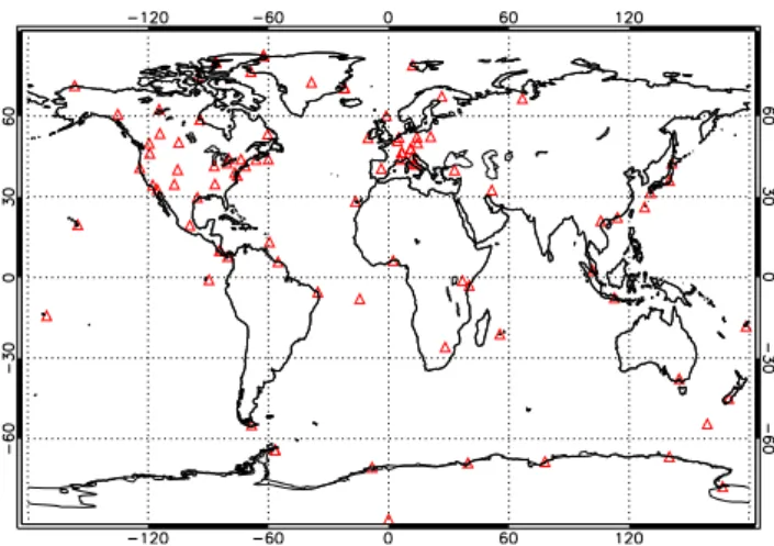
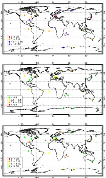
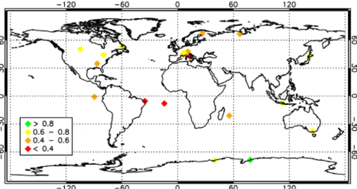
The geographical distribution of the ozonesonde stations whose data were used to create the dataset is shown in Fig. 1. The ozone soundings were colocated with OML1BRUG data according to the overpass info provided by the Aura Val-idation Data Center (AVDC) for the OMTO3 Level 2 prod-uct. The following procedure was followed in performing the colocations:
1. For each ozone sounding, the OML1BRUG files corre-sponding to the overpass orbits indicated in the AVDC info were selected.
2. For each OML1BRUG file, the OMI pixel having its center closest to the ozonesonde station was selected as a candidate for the colocation.
3. The candidate pixel was discarded if its center and the station coordinates were more than 1◦ apart in latitude or longitude or separated by more than 6 h in time. Such colocation criteria were adopted in order to be rea-sonably sure that the tropospheric air volumes sampled by OMI were representative of the volume actually covered by the corresponding ozone soundings.
3.3 Preprocessing of OMI spectral measurements
The OML1BRUG radiance spectra were converted in top-of-atmosphere (TOA) reflectance spectra by normalization to OML1BIRR irradiance spectra and cosine of the SZA. A nat-ural logarithm was then applied to the computed reflectances. The following preprocessing steps were applied in order to compute the TOA reflectance spectra:
1. The quality of each radiance and irradiance spectral pixel was checked with respect to the OMI L1B quality flags, according to the guidelines given in van den Oord and Veefkind (2002). The spectral pixels that failed the quality test were discarded from the subsequent compu-tations.
2. The spectra whose number of discarded wavelengths exceeded the 5 % of the total were discarded, and were not used in the colocation procedure.
3. The radiance and irradiance spectra that survived this screening procedure were linearly interpolated on a 0.1 nm wide common spectral grid. The linear interpola-tion has been chosen over more sophisticated techniques (e.g., cubic spline interpolation) because it is computa-tionally less demanding.
Fig. 1.Spatial distribution of the ozonesonde stations used to con-struct the dataset to train and test the NN.
4. The TOA reflectance spectra were computed using the interpolated radiance and irradiance spectra, and the natural logarithm of the resulting values was computed. As for the quality-flag-based filtering, particular care was taken in order to exclude pixels affected by row anomaly from the dataset. According to the information available from the Royal Dutch Meteorological Institute (KNMI), the row anomaly started to appear on 25 June 2007, affect-ing the rows 53–54 (0 based) in the OMI across-track di-rection. After about one year, it expanded to the rows 37– 44, and began to assume an erratic behavior after 24 Jan-uary 2009, randomly affecting subsets of the rows 24–59. Additional information about the row anomaly effect in OMI can be found at the webpage www.knmi.nl/omi/research/ product/rowanomaly-background.php. According to this in-formation, the flagging of row anomaly events in the OMI Level 1B products was not complete until 1 February 2010. Therefore, it was decided to exclude from the dataset all the OMI measurements over the rows 24–59 starting from 24 January 2009 in order to be reasonably sure that the test statistics did not contain contaminated pixels.
Apart from the filtering based on the quality flags, other screening actions were performed in order to strengthen the quality of the dataset. Specifically, pixels having cloud frac-tions larger than 0.3 were discarded. The choice of 0.3 as a threshold for the cloud fraction was made to establish a trade-off between the need of excluding pixels that are excessively affected by clouds and the need of ensuring an adequate num-ber of samples to train the NN and assess its performance in a wide range of situations.
2011). Therefore, the information content of the computed log-reflectance spectra can be considerably compressed through a data dimensionality reduction technique. In this work a simple linear PCA was used. In order to choose an appropriate value for the number of principal components (PCs) to retain after the PCA procedure, the error in the reconstruction of the log-reflectance spectra from the com-pressed spectra was monitored as a function of the number of retained PCs. This procedure led to retainment of 20 PCs since adding further PCs did not improve the reconstruction significantly (reflectance reconstruction RMS error of about 0.01 %).
4 Design of the neural network
4.1 Training, validation, and test subsets
The colocation procedure described in the previous section has led to the generation of 10 017 input–output pairs. Such pairs were used to train the NN algorithm and assess its per-formance with data not used during the training phase. The network was trained using only colocations that cover the pe-riod from 2004 to 2008. This choice was made in order to set aside enough data to test the NN behavior outside the training period. The dataset was split into four subsets:
i. 5489 pairs were used to train the NN;
ii. 1737 pairs were used to determine when to stop the training process via early stopping cross-validation (see Sect. 2.4);
iii. 2071 pairs were used to evaluate the generalization of the trained NN during the training period;
iv. 720 pairs were used to evaluate the trained NN general-ization outside the training period.
From now on these four datasets will be referred to asDtrain, Dvalid, Dtest1 and Dtest2, respectively. The union between Dtest1andDtest2will be indicated asDtest.
In order to ensure the independence between the datasets, without affecting their comprehensiveness, the data were as-signed to each set based on the ozonesonde station they re-ferred to. Stations used in the training dataset were not used for the test and validation datasets. A significant number of colocations pertaining to the different latitudinal bands were present in each subset.
4.2 Input preprocessing
The input vector of the OMITROPO3-NN consists of 43 in-puts: 20 PCs of the reflectance spectra, SZA, VZA, terrain height, NCEP/NCAR temperature profiles at 17 pressure lev-els, NCEP/NCAR tropopause pressure, radiative cloud frac-tion, and monthly mean TCO. A logistic activation function was chosen for the hidden and the output layers of the NN.
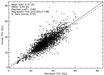
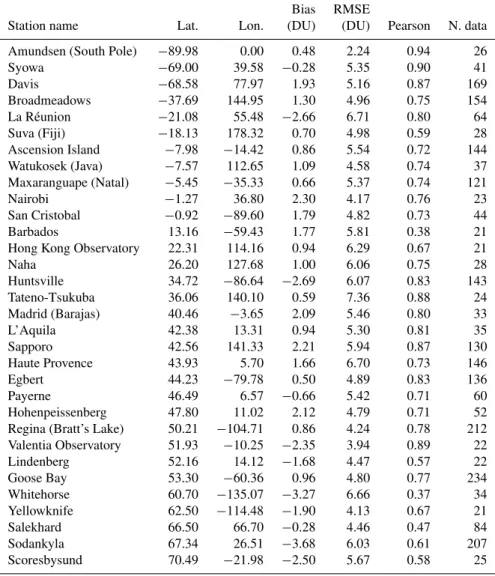
Fig. 2.Overall validation results, obtained both during and after the time period covered by the training set.
Before proceeding with the NN training, a further prepro-cessing step was applied to the input and target data in order to make them compatible with the mathematical properties of the logistic function. Specifically, since the output of the logistic function lies between 0 and 1, a linear scaling be-tween these values was applied to the TCO data. Similarly, all the input data were linearly scaled between−1 and 1 in order to avoid the saturation of the hidden neurons after the initialization of the NN weights.
4.3 Training and architecture selection
The NN was trained using the scaled conjugate gradient (SCG) learning algorithm (Møller, 1993). A heuristic pro-cedure, as described in Sect. 2.4, was adopted to select the number of hidden layers and neurons. The selected NN ar-chitecture has one hidden layer with 5 neurons inside. For this architecture, the training was stopped after about 1000 cycles, using early stopping cross-validation.
5 Results
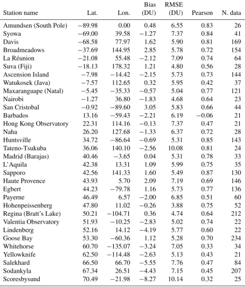
Fig. 3.Histograms of the absolute (top) and relative (bottom) dif-ferences between the retrieved and the target tropospheric ozone columns.
5.1 Generalization during and after the training period
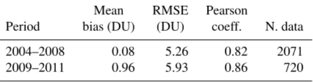
It is important to understand whether there are any differ-ences in the performances of the algorithm between the years covered by the training set and those not covered by it as this may provide an indication on the degree of robustness of the NN with respect to changes of the instrumental response. Separate error statistics were computed for theDtest1, con-taining examples percon-taining to the period between 2004 and 2008 and theDtest2 sets, consisting of examples acquired af-ter 2008. The results are summarized in Table 2.
The statistics of the comparison between the NN sults and the sonde observations are similar to the re-sults for the training period (bias smaller than 1 DU, RMSE smaller than 6 DU, correlation coefficient larger than 0.8). These results indicate that applying the NN to OMI data acquired after the period covered by the training set should not result in a significant performance degradation of the algorithm. This is consistent with the very good
Table 2.Retrieval results during and after the period covered by the training set. The training set covers the period from 2004 to 2008.
Mean RMSE Pearson
Period bias (DU) (DU) coeff. N. data
2004–2008 0.08 5.26 0.82 2071
2009–2011 0.96 5.93 0.86 720
Table 3.Retrieval results on the test set, stratified by latitude band.
Mean RMSE Pearson
Latitude band bias (DU) (DU) coeff. N. data
90◦S–60◦S 1.99 5.63 0.86 271
60◦S–30◦S 1.45 5.22 0.76 181
30◦S–30◦N 0.59 5.65 0.80 611
30◦N–60◦N 0.52 5.28 0.82 1357
60◦N–90◦N −2.69 5.66 0.54 371
radiometric stability displayed by OMI throughout its op-erational lifetime. Details about the OMI calibration status can be found at the webpage www.knmi.nl/omi/research/ calibration/instrument_status_v3/perf_plots/index.html.
5.2 Geographical features in the retrieval algorithm
The performances of the algorithm were evaluated after strat-ifying theDtestset by latitude zone. Five zones were defined: Antarctica (latitude between 90◦S and 60◦S), southern mid-latitudes (60◦S to 30◦S), tropics (30◦S to 30◦N), north-ern midlatitudes (30◦N to 60◦N) and the Arctic (60◦N to 90◦N).
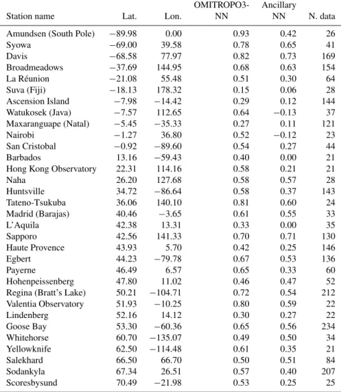
Maps of mean biases, Pearson correlation coefficients, and RMSEs found over the ozonesonde stations having at least 35 measurements included in the test dataset are shown in Fig. 4.
The performances of the algorithm, in terms of mean bias, RMSE and Pearson coefficient, are comparable for four of the five zones. Only for the Arctic region the bias was larger. The causes of this bias are currently under study. A possible reason might lie in artifacts related to the occasionally diffi-cult definition of the tropopause in this region.The results are summarized in Table 3.
Fig. 4.Mean bias (top), Pearson correlation coefficient (middle), and RMS difference (bottom) between ozonesonde measurements and retrievals for all the measurement stations having at least 35 measurements in the test dataset.
Scatter plots and time series of the “true” and retrieved TCO as a function of the day of year (DOY) for the sta-tions Broadmeadows (Australia) and Goose Bay (Canada) are shown in Figs. 5 and 6 as examples. Similar plots for other stations can be found in the supplementary informa-tion.
5.3 Non-climatological features
An important question is to what extent is the algorithm ca-pable of recognizing anomalous events, i.e., cases of large departures of the actual TCO from its climatological value used as an a priori for the retrieval. In order to investigate this aspect, a TCO relative anomaly was defined as the per-cent difference between the actual TCO and its climatologi-cal value taken from the Ziemke climatology, and the differ-ence between the retrieved and the actual TCO anomalies
Fig. 5.Scatter plot (top) and time series (bottom) of retrieved and ozonesonde TCO at Broadmeadows (Australia).
were analyzed. The results on the Dtest set are plotted in Fig. 7. The correlation coefficient between the actual and the retrieved TCO anomalies is smaller than the correlation found between the TCO absolute values. Nevertheless, there still exists reasonable agreement between the actual and the retrieved anomalies, as correlations decreased only from 0.83 to 0.72, indicating that the algorithm uses information other than the a priori in order to perform its retrievals. Such in-formation comes from the satellite measurements as well as from the reanalysis data provided as inputs for the NN. An at-tempt to investigate the relative contribution of satellite mea-surements and satellite data to the retrieved TCOs is made in the next subsection.
Table 4.Retrieval validation results divided by station, sorted by increasing latitude. Only stations with at least 20 measurements included
in theDtestset were considered.
Bias RMSE
Station name Lat. Lon. (DU) (DU) Pearson N. data
Amundsen (South Pole) −89.98 0.00 0.48 2.24 0.94 26
Syowa −69.00 39.58 −0.28 5.35 0.90 41
Davis −68.58 77.97 1.93 5.16 0.87 169
Broadmeadows −37.69 144.95 1.30 4.96 0.75 154
La Réunion −21.08 55.48 −2.66 6.71 0.80 64
Suva (Fiji) −18.13 178.32 0.70 4.98 0.59 28
Ascension Island −7.98 −14.42 0.86 5.54 0.72 144
Watukosek (Java) −7.57 112.65 1.09 4.58 0.74 37
Maxaranguape (Natal) −5.45 −35.33 0.66 5.37 0.74 121
Nairobi −1.27 36.80 2.30 4.17 0.76 23
San Cristobal −0.92 −89.60 1.79 4.82 0.73 44
Barbados 13.16 −59.43 1.77 5.81 0.38 21
Hong Kong Observatory 22.31 114.16 0.94 6.29 0.67 21
Naha 26.20 127.68 1.00 6.06 0.75 28
Huntsville 34.72 −86.64 −2.69 6.07 0.83 143
Tateno-Tsukuba 36.06 140.10 0.59 7.36 0.88 24
Madrid (Barajas) 40.46 −3.65 2.09 5.46 0.80 33
L’Aquila 42.38 13.31 0.94 5.30 0.81 35
Sapporo 42.56 141.33 2.21 5.94 0.87 130
Haute Provence 43.93 5.70 1.66 6.70 0.73 146
Egbert 44.23 −79.78 0.50 4.89 0.83 136
Payerne 46.49 6.57 −0.66 5.42 0.71 60
Hohenpeissenberg 47.80 11.02 2.12 4.79 0.71 52
Regina (Bratt’s Lake) 50.21 −104.71 0.86 4.24 0.78 212
Valentia Observatory 51.93 −10.25 −2.35 3.94 0.89 22
Lindenberg 52.16 14.12 −1.68 4.47 0.57 22
Goose Bay 53.30 −60.36 0.96 4.80 0.77 234
Whitehorse 60.70 −135.07 −3.27 6.66 0.37 34
Yellowknife 62.50 −114.48 −1.90 4.13 0.67 21
Salekhard 66.50 66.70 −0.28 4.46 0.47 84
Sodankyla 67.34 26.51 −3.68 6.03 0.61 207
Scoresbysund 70.49 −21.98 −2.50 5.67 0.58 25
This could be related to the limited availability of training data in the tropics. However, it must be kept in mind that a precise TCO anomaly estimation in the tropics is a challeng-ing task because the range of the anomalies over this area is usually small.
5.4 Contribution of OMI reflectances to the retrieved TCO
Given the large amount of ancillary data used by the OMITROPO3-NN, many of which are correlated with the TCO, it is important to evaluate to what extent using OMI reflectances improves the results with respect to using only the ancillary data themselves in a regression. Some insight on this point can be obtained by training a second NN using only the ancillary data as inputs. This second network achieved a RMSE of 6.11 DU on the test set, with a correlation coef-ficient of 0.78. The results divided by station are shown in
Table 5.Results for the NN trained without OMI reflectances, divided by station, sorted by increasing latitude. Only stations with at least 20
measurements included in theDtestset were considered.
Bias RMSE
Station name Lat. Lon. (DU) (DU) Pearson N. data
Amundsen (South Pole) −89.98 0.00 0.48 6.55 0.83 26
Syowa −69.00 39.58 −1.27 7.37 0.84 41
Davis −68.58 77.97 1.62 5.90 0.81 169
Broadmeadows −37.69 144.95 2.85 5.78 0.72 154
La Réunion −21.08 55.48 −2.12 7.09 0.74 64
Suva (Fiji) −18.13 178.32 1.21 4.80 0.56 28
Ascension Island −7.98 −14.42 −2.15 5.73 0.73 144
Watukosek (Java) −7.57 112.65 0.32 5.95 0.42 37
Maxaranguape (Natal) −5.45 −35.33 −0.57 5.04 0.77 121
Nairobi −1.27 36.80 −1.83 4.68 0.64 23
San Cristobal −0.92 −89.60 3.05 5.83 0.66 44
Barbados 13.16 −59.43 −2.21 6.19 −0.06 21
Hong Kong Observatory 22.31 114.16 −0.13 7.37 0.47 21
Naha 26.20 127.68 −1.33 6.37 0.72 28
Huntsville 34.72 −86.64 −0.69 5.31 0.85 143
Tateno-Tsukuba 36.06 140.10 −2.56 10.08 0.81 24
Madrid (Barajas) 40.46 −3.65 0.04 5.31 0.78 33
L’Aquila 42.38 13.31 1.09 5.99 0.75 35
Sapporo 42.56 141.33 1.60 5.49 0.87 130
Haute Provence 43.93 5.70 2.09 7.19 0.69 146
Egbert 44.23 −79.78 1.16 5.73 0.77 136
Payerne 46.49 6.57 −2.00 6.85 0.51 60
Hohenpeissenberg 47.80 11.02 −0.26 3.88 0.75 52
Regina (Bratt’s Lake) 50.21 −104.71 0.36 4.74 0.64 212
Valentia Observatory 51.93 −10.25 −2.83 5.02 0.74 22
Lindenberg 52.16 14.12 −4.19 5.77 0.60 22
Goose Bay 53.30 −60.36 1.12 5.28 0.70 234
Whitehorse 60.70 −135.07 −3.24 7.05 0.33 34
Yellowknife 62.50 −114.48 −2.63 5.13 0.43 21
Salekhard 66.50 66.70 −5.55 7.76 0.47 84
Sodankyla 67.34 26.51 −4.43 7.15 0.45 207
Scoresbysund 70.49 −21.98 −8.27 10.14 0.32 25
coefficients between the two NNs for all the ozonesonde stations with at least 20 measurements. Again, it can be seen that the performances of the OMITROPO3-NN with re-spect to this parameter are considerably better than those of the NN trained without OMI reflectances for almost all the ozonesonde stations.
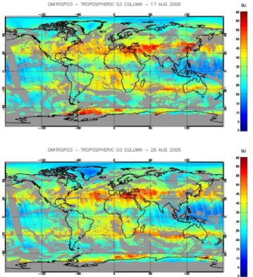
6 Examples: 17 and 26 August 2006
6.1 Global retrievals
Besides carrying out a validation against ozonesondes, it is important to see how reasonable are the TCO spatial patterns obtained by applying the OMITROPO3-NN to an extended area (e.g., an OMI orbit, or the entire globe). In this section, two examples of global TCO retrievals are discussed.
Table 6.Pearson correlation coefficients between observed and estimated TCO anomalies for the OMITROPO3-NN and for the NN trained
without OMI reflectances, divided by station, sorted by increasing latitude. Only stations with at least 20 measurements included in theDtest
set were considered.
OMITROPO3- Ancillary
Station name Lat. Lon. NN NN N. data
Amundsen (South Pole) −89.98 0.00 0.93 0.42 26
Syowa −69.00 39.58 0.78 0.65 41
Davis −68.58 77.97 0.82 0.73 169
Broadmeadows −37.69 144.95 0.68 0.63 154
La Réunion −21.08 55.48 0.51 0.30 64
Suva (Fiji) −18.13 178.32 0.15 0.06 28
Ascension Island −7.98 −14.42 0.29 0.12 144
Watukosek (Java) −7.57 112.65 0.64 −0.13 37
Maxaranguape (Natal) −5.45 −35.33 0.27 0.11 121
Nairobi −1.27 36.80 0.52 −0.12 23
San Cristobal −0.92 −89.60 0.54 0.27 44
Barbados 13.16 −59.43 0.40 0.00 21
Hong Kong Observatory 22.31 114.16 0.58 0.21 21
Naha 26.20 127.68 0.58 0.57 28
Huntsville 34.72 −86.64 0.58 0.37 143
Tateno-Tsukuba 36.06 140.10 0.81 0.60 24
Madrid (Barajas) 40.46 −3.65 0.61 0.55 33
L’Aquila 42.38 13.31 0.33 0.00 35
Sapporo 42.56 141.33 0.70 0.71 130
Haute Provence 43.93 5.70 0.42 0.25 146
Egbert 44.23 −79.78 0.67 0.53 136
Payerne 46.49 6.57 0.65 0.33 60
Hohenpeissenberg 47.80 11.02 0.46 0.47 52
Regina (Bratt’s Lake) 50.21 −104.71 0.72 0.54 212
Valentia Observatory 51.93 −10.25 0.80 0.59 22
Lindenberg 52.16 14.12 0.30 0.27 22
Goose Bay 53.30 −60.36 0.65 0.56 234
Whitehorse 60.70 −135.07 0.49 0.50 34
Yellowknife 62.50 −114.48 0.61 0.35 21
Salekhard 66.50 66.70 0.50 0.51 84
Sodankyla 67.34 26.51 0.57 0.40 207
Scoresbysund 70.49 −21.98 0.53 0.25 25
because also the radiometric calibration of the OMI radiances contributes to the striping effect.
Another feature that sometimes appears is represented by some abrupt meridional gradients in the retrieved TCOs (see, e.g., the northern edge of the “red” region in the Central Asia on 17 August 2006, above panel in Fig. 10). This might be due to the coarse resolution of either the tropopause or the a priori fields used as inputs in the OMITROPO3-NN.
The day of 26 August has been chosen as a sample date also because it allows a visual comparison with a TCO map shown in the paper by Liu et al. (2010). For the reader’s convenience, such a map is reported in Fig. 11. A similar color scale was used in Figs. 10 and 11 in order to facili-tate visual comparisons. For instance, it can be noticed that the ozone peak between southern Brazil, northern Argentina, and Paraguay is reproduced quite well by the OMITROPO3-NN algorithm. The same holds for the high-ozone areas
around the Azores, the Eastern coast of the United States, the Black Sea, off the coast of southwestern Africa and south of Madagascar. Also, the ozone patterns over Australia look similar. The main differences exist over North Africa, where the OMITROPO3-NN seems to yield larger ozone values, and over Central Asia, where the OMITROPO3-NN seems to yield a more extended area of large TCO than Liu et al. (2010). Unfortunately, no correlative measurements over these areas were found to assess which of the two al-gorithms performed better.
6.2 Comparisons with the TM5 chemistry/transport
model
Fig. 6.Scatter plot (top) and time series (bottom) of retrieved and ozonesonde TCO at Goose Bay (Canada).
Fig. 7.Comparison between actual and estimated TCO anomaly.
(CTM) TM5 (Krol et al., 2005; Williams et al., 2012). The model provided simulated ozone fields at 34 pressure lev-els, on a grid of 3◦in longitude by 2◦in latitude. In order
Fig. 8.Pearson correlation coefficient between actual and estimated TCO anomalies for all the measurement stations having at least 35 measurements included in the test set.
Fig. 9.Comparison between actual and estimated TCO anomaly for the NN trained only with ancillary data.
to perform the comparison, both the NCEP tropopause pres-sure and the TCO fields retrieved by the OMITROPO3-NN were mapped on the same grid. The remapping has been done by selecting all the OMI pixels whose center lie within each TM5 grid cell, and associating the median non-missing TCO to the cell. The NCEP tropopause pressure was used as upper integration limit for the TM5 simulated ozone profiles.
The TCO fields simulated using TM5 on the two dates are shown in Fig. 12, and scatter plots of modeled versus re-trieved TCOs are shown in Fig. 13. Such statistics show that the OMITROPO3-NN has a positive bias of about 4 DU with respect to TM5. The Pearson correlation coefficient between the TCO fields is slightly larger than 0.80 for both the dates. The structure of the differences between the OMITROPO3-NN and the TM5 estimates is shown with more detail in Fig. 14, where the histograms of the absolute differences for the two dates are depicted.
Figure 15 shows a map of the NN-TM5 absolute differ-ences for the two dates under study.
Fig. 10. Global tropospheric ozone fields retrieved by the OMITROPO3-NN algorithm on 17 (top) and 26 August (bottom) 2006. No retrieval is performed on pixels with cloud fraction larger than 30 %.
Fig. 11. Global tropospheric ozone field on 26 August 2006 as shown in Liu et al. (2010). From http://www.cfa.harvard.edu/ atmosphere/ozone_tropo.html.
higher TCO values than TM5 are regularly retrieved by the OMITROPO3-NN over the southern midlatitudes. The un-derestimations are mostly concentrated between the tropics and, to a lesser extent, over Central Europe and the eastern United States. Large underestimations occur over southeast-ern Asia.
Similar analyses performed during individual days in Oc-tober 2006 gave similar results (Di Noia et al., 2012a,b).
Fig. 12.Global tropospheric ozone fields simulated by the TM5 CTM on August 17 (top) and 26 August (bottom) 2006.
6.3 Retrieval sensitivity to tropopause pressure
Whenever a retrieval algorithm is developed, it is important to assess its sensitivity to its input quantities. In the case of NNs, a powerful way to do this is represented by the analy-sis of the NN input Jacobians, i.e., the derivatives of the NN model8W∗with respect to its inputsx. An important prop-erty of single hidden layer NNs is that their input Jacobians can be written analytically (Blackwell and Chen, 2009).
Since NN mappings are nonlinear, a difficulty in using their Jacobians for sensitivity analyses lies in the fact that they are input dependent. One method to overcome this dif-ficulty is to use the Jacobian to define a NN sensitivity factor (SF) of an outputyj with respect to an inputxi as the ratio
between the fractional change ofyjwith respect to its actual
value, and the corresponding fractional change ofxi:
SFj(xi)= dyj/yj
dxi/xi
= xi
yj
·dyj
dxi
. (8)
Fig. 13.Scatter plots of the OMITROPO3-NN retrievals versus the TM5 TCO simulations on 17 (top) and 26 August (bottom) 2006. The OMITROPO3-NN TCO fields are remapped on the TM5 grid.
Two maps of the algorithm SF with respect to the tropopause pressure – for 17 and 26 August 2006 – are shown in Fig. 16. It can be seen that the SF always assumes negative values. This result is reasonable because it indicates that the negative correlation between tropopause pressure and TCO is captured by the NN model. Furthermore, the SF absolute val-ues tend to increase going from the tropics toward the poles. An increase of |SF| indicates a larger sensitivity of the re-trieved TCO to the tropopause pressure. The increase in|SF|
is not symmetric with respect to the Equator because of the motion of the Intertropical Convergence Zone (ITCZ) with the season. This could be an indication that the retrievals at midlatitudes are more sensitive to the tropopause pressure during winter.
7 Conclusions
A new neural network algorithm to retrieve tropo-spheric ozone from OMI data at global scale – named
Fig. 14. Histograms of the absolute differences between the OMITROPO3-NN retrievals and the TM5 TCO simulations on 17 (top) and 26 August (bottom) 2006. The OMITROPO3-NN TCO fields are remapped on the TM5 grid.
NN – has been presented. The OMITROPO3-NN inherits from previous work and adds novel character-istics like the global coverage, the use of tropopause infor-mation to better demarcate the actual troposphere, and the incorporation of ancillary data and a priori information into the NN input vector in order to improve the retrieval accu-racy. As a result, the OMITROPO3-NN provides daily global estimates of the tropospheric ozone column.
The algorithm has been validated against ozonesondes and CTM simulations, and encouraging results have been ob-tained. Overall, the NN appears to be capable of determining the spatial and temporal TCO variability.
Fig. 15.Maps of the absolute differences between OMITROPO3-NN and TM5 TCO fields on 17 (top) and 26 August (bottom) 2006. The OMITROPO3-NN TCO fields are remapped on the TM5 grid.
also after the training period, even though a slight increase in the global retrieval bias seems to be present.
Over all the latitude bands except the Arctic, a relatively low bias against the ozonesonde measurements was noticed. The correlation coefficients between retrieved and measured tropospheric ozone columns range approximately between 0.75 and 0.85, and the RMS errors are between 5 and 6 DU. On the other hand, over the Arctic a larger negative bias was detected, whose cause is a topic of ongoing research.
The ozonesonde data were also used in order to assess the capability of the OMITROPO3-NN to detect and estimate departures of the tropospheric ozone columns from their cli-matological values. A global correlation coefficient of about 0.70 was found between the actual and the retrieved relative anomalies. A geographical analysis of this correlation coef-ficient seems to suggest that the anomaly estimation capabil-ity of the OMITROPO3-NN over the tropics is worse than at other latitudes. This may indicate that an insufficient training was obtained in this latitude band due to the relatively low number of available ozonesonde data. Future versions of the algorithm will have to address this problem properly. A pos-sible approach may consist of complementing ozonesonde data with radiative transfer simulations in tropical scenar-ios. Another alternative is the relaxation of colocation criteria over the tropics.
In order to assess the contribution of OMI reflectances to the retrievals, a second NN was trained using only the
Fig. 16.Global fields of the tropopause sensitivity factor computed for the OMITROPO3-NN algorithm on 17 (top) and 26 August (bot-tom) 2006.
ancillary data. The estimation capabilities of this second NN were shown to be worse than those of the OMITROPO3-NN, especially in the estimation of TCO anomalies.
After the comparison with ozonesonde data, examples of operational use of the OMITROPO3-NN were provided. The tropospheric ozone fields retrieved by the OMITROPO3-NN in two dates during August 2006 were compared with simu-lations made with the TM5 CTM. Such comparisons suggest that the OMITROPO3-NN has a bias of about 4 DU with re-spect to TM5. However, the differences between retrieved and simulated tropospheric ozone fields exhibit a peculiar geographic pattern, with the OMITROPO3-NN that over-estimates TM5 simulations over southern midlatitudes and underestimates between the tropics. Despite this, the simu-lated global spatial patterns are fairly well reproduced by the OMITROPO3-NN, as shown by the correlation coefficients, which are higher than 0.80.
applied to evaluate the NN sensitivity to all the input quanti-ties for every retrieval.
While the OMITROPO3-NN generally shows high cor-relations and low RMS errors with respect to ozoneson-des compared to other existing satellite products (Schoeberl et al., 2007; Thompson et al., 2012), a possible drawback of the current version of the algorithm is its massive use of ancillary information to complement the OMI radiomet-ric measurements. This was necessary in order to constrain the retrieval problem properly as UV measurements may not have enough sensitivity to directly retrieve tropospheric ozone without a priori constraints.
Supplementary material related to this article is available online at: http://www.atmos-meas-tech.net/6/ 895/2013/amt-6-895-2013-supplement.zip.
Acknowledgements. All the PIs of the ozonesonde stations whose data were used in this work are gratefully acknowledged. WOUDC, NDACC and SHADOZ data have been downloaded from the re-spective websites, and are publicly available. The NCEP Reanaly-sis data are provided by the NOAA/OAR/ESRL PSD, Boulder, Col-orado, USA, from their website at http://www.esrl.noaa.gov/psd/.
ISAC-CNR, ReSMA-Italian Air Force and CETEMPS are acknowl-edged for the provision of Italian ozonesonde data. The ozone mon-itoring activities of CETEMPS are partly funded by the Italian Min-istero dell’Ambiente e della Tutela del Territorio e del Mare.
Marco Iarlori (CETEMPS) is gratefully acknowledged for his help with L’Aquila ozonesonde station data, Marco Cervino (ISAC-CNR) is gratefully acknowledged for his help with San Pietro Capofiume ozonesonde station data. Stefania Vergari and Emanuele Vuerich (ReSMA, Italian Air Force) are gratefully ac-knowledged for their help with Vigna di Valle ozonesonde data. Michael Yan (NASA Aura Validation Data Center) is gratefully ac-knowledged for providing the OMTO3 overpass files for the sta-tions Barbados, Maxaranguape, Whitehorse and Yellowknife upon request.
The three anonymous reviewers are gratefully acknowledged for their constructive comments. ADN would like to thank sev-eral people from the Royal Netherlands Meteorological Institute, for valuable discussions that helped improve the paper significantly.
Edited by: P. K. Bhartia
References
Ahn, C., Ziemke, J. R., Chandra, S., and Bhartia, P. K.: Derivation of tropospheric column ozone from the Earth Probe TOMS/GOES co-located data sets using the cloud slicing technique, J. Atmos. Sol.-Terr. Phy., 65, 1127–1137, doi:10.1016/S1364-6826(03)00166-4, 2003.
Aires, F., Prigent, C., Rossow, W. B., and Rothstein, M.: A new neural network approach including first-guess for retrieval
of atmospheric water vapor, cloud liquid water path, sur-face temperature and emissivities over land from satellite mi-crowave observations, J. Geophys. Res., 106, 14887–14907, doi:10.1029/2001JD900085, 2001.
Aires, F., Prigent, C., and Rossow, W. B.: Neural network uncer-tainty assessment using Bayesian statistics with application to remote sensing: 2. Output errors, J. Geophys. Res., 109, D10304, doi:10.1029/2003JD004174, 2004a.
Aires, F., Prigent, C., and Rossow, W. B.: Neural network uncer-tainty assessment using Bayesian statistics with application to remote sensing: 3. Network Jacobians, J. Geophys. Res., 109, D10305, doi:10.1029/2003JD004175, 2004b.
Akaike, H.: Information theory and an extension of the maximum likelihood principle, in: Proceedings of the 2nd International Symposium on Information Theory, Vol. 1, 267–281, Akademiai Kiado, Budapest, 1973.
Bhartia, P. K. and Wellemeyer, C.: TOMS-V8 total O3algorithm,
in: OMI Ozone Product, OMI-ATBD-02, edited by: Bhartia, P. K., Vol. 2, Chap. 2, 15–31, NASA Goddard Space Flight Cen-ter, Greenbelt, MD, USA, 2002.
Bishop, C. M.: Neural Networks for Pattern Recognition, Oxford University Press, New York, NY, USA, 1995.
Blackwell, W. J.: A Neural-Network technique for the retrieval of atmospheric temperature and moisture profiles from high spec-tral resolution sounding data, IEEE Trans. Geosci. Remote Sens., 43, 2535–2546, doi:10.1109/TGRS.2005.855071, 2005. Blackwell, W. J. and Chen, F. W.: Neural Networks in Atmospheric
Remote Sensing, Artech House, Norwood, MA, USA, 2009. Carmichael, G. R., Uno, I., Phadnis, M. J., Zhang, Y., and
Sun-woo, Y.: Tropospheric ozone production and transport in the springtime in east Asia, J. Geophys. Res., 103, 10649–10671, doi:10.1029/97JD03740, 1998.
Chameides, W. and Walker, J. C. G.: A photochemical the-ory of tropospheric ozone, J. Geophys. Res., 78, 8751–8760, doi:10.1029/JC078i036p08751, 1973.
Chance, K. V., Burrows, J. P., Perner, D., and Schneider, W.: Satellite measurements of atmospheric ozone profiles, in-cluding tropospheric ozone, from ultraviolet/visible measure-ments in the nadir geometry: A potential method to retrieve tropospheric ozone, J. Quant. Spectrosc. Ra., 57, 467–476, doi:10.1016/S0022-4073(96)00157-4, 1997.
Chevallier, F., Chéruy, F., Scott, N. A., and Chédin, A.: A neural network approach for a fast and accurate computation of a longwave radiative budget, J. Appl. Meteor., 37, 1385–1397, doi:10.1175/1520-0450(1998)037<1385:ANNAFA>2.0.CO;2, 1998.
Chevallier, F., Morcrette, J.-F., Chéruy, F., and Scott, N. A.: Use of a neural-network-based long-wave radiative-transfer scheme in the ECMWF atmospheric model, Q. J. Roy. Meteorol. Soc., 126, 761–776, doi:10.1002/qj.49712656318, 2000.
Creilson, J. K., Fishman, J., and Wozniak, A. E.: Intercontinental transport of tropospheric ozone: a study of its seasonal variabil-ity across the North Atlantic utilizing tropospheric ozone resid-uals and its relationship to the North Atlantic Oscillation, At-mos. Chem. Phys., 3, 2053–2066, doi:10.5194/acp-3-2053-2003, 2003.
Cybenko, G.: Approximation by superpositions of a
sig-moidal function, Math. Control Signal, 2, 303–314,
de Laat, A. T. J., Aben, I., and Roelofs, G. J.: A model
perspec-tive on total tropospheric O3 column variability and
implica-tions for satellite observaimplica-tions, J. Geophys. Res., 110, D13303, doi:10.1029/2004JD005264, 2005.
Del Frate, F., Ortenzi, A., Casadio, S., and Zehner, C.: Application of neural algorithms for a real-time estimation of ozone profiles from GOME measurements, IEEE T. Geosci. Remote, 40, 2263– 2270, doi:10.1109/TGRS.2002.803622, 2002.
Del Frate, F., Iapaolo, M., and Casadio, S.: Intercomparison be-tween GOME ozone profiles retrieved by neural network inver-sion schemes and ILAS products, J. Atmos. Ocean. Tech., 22, 1433–1440, doi:10.1175/JTECH1764.1, 2005a.
Del Frate, F., Iapaolo, M., Casadio, S., Godin-Beekmann, S., and Petitdidier, M.: Neural networks for the dimensional-ity reduction of GOME measurement vector in the estima-tion of ozone profiles, J. Quant. Spectrosc. Ra., 92, 275–291, doi:10.1016/j.jqsrt.2004.07.028, 2005b.
Di Noia, A., Sellitto, P., Del Frate, F., and de Laat, J.: Global tro-pospheric ozone retrievals from OMI data by means of neural networks, in: Proceedings of ESA Atmospheric Science Confer-ence 2012, Bruges, Belgium, 18–22 June 2012, 2012a.
Di Noia, A., Sellitto, P., Del Frate, F., and de Laat, J.: A neural network algorithm to retrieve tropospheric ozone from the Ozone Monitoring Instrument: Design and validation, in: Proceedings of the 9th International Symposium on Tropospheric Profiling, L’Aquila, Italy, 3–7 September 2012, 2012b.
Di Noia, A., Sellitto, P., Del Frate, F., Cervino, M., Iarlori, M., and Rizi, V.: Tropospheric ozone column retrieval from OMI data by means of neural networks: A validation exercise with ozone soundings over Europe, EURASIP J. Adv. Sig. Pr., 21, doi:10.1186/1687-6180-2013-21, 2013.
Doicu, A., Trautmann, T., and Schreier, F.: Numerical Regulariza-tion for Atmospheric Inverse Problems, Springer, Dordrecht, the Netherlands, 2010.
Dybowski, R. and Roberts, S. J.: Confidence intervals and predic-tion intervals for feedforward neural networks, in: Clinical Ap-plications of Artificial Neural Networks, edited by: Dybowski, R., Chap. 13, 298–326, Cambridge University Press, Cambridge, UK, doi:10.1017/CBO9780511543494.013, 2009.
Fishman, J.: Observing tropospheric ozone from space, Prog. Envi-ron. Sci., 2, 275–290, 2000.
Fishman, J. and Larsen, J. C.: Distribution of total ozone and stratospheric ozone in the tropics: Implications for the distribu-tion of tropospheric ozone, J. Geophys. Res., 92, 6627–6634, doi:10.1029/JD092iD06p06627, 1987.
Fishman, J., Minnis, P., and Reichle Jr., H. G.: Use of satellite data to study tropospheric ozone in the tropics, J. Geophys. Res, 91, 14451–14465, doi:10.1029/JD091iD13p14451, 1986.
Fishman, J., Vukovich, F. M., Cahoon, D. R., and Shipham, M. C.: The characterization of an air pollution episode using satellite to-tal ozone measurements, J. Clim. Appl. Meteor., 26, 1638–1654, doi:10.1175/1520-0450(1987)026<1638:TCOAAP>2.0.CO;2, 1987.
Fortuin, J. P. F. and Kelder, H.: An ozone climatology based on ozonesonde and satellite measurements, J. Geophys. Res., 103, 31079–31734, doi:10.1029/1998JD200008, 1998.
Funahashi, K.-I.: On the approximate realization of continuous mappings by neural networks, Neural Networks, 2, 183–192, doi:10.1016/0893-6080(89)90003-8, 1989.
Geman, S., Bienenstock, E., and Doursat, R.: Neural networks and the bias/variance dilemma, Neural Comput., 4, 1–58, doi:10.1162/neco.1992.4.1.1, 1992.
Göttsche, F.-M. and Olesen, F. S.: Evolution of neural net-works for radiative transfer calculations in the terrestrial in-frared, Remote Sens. Environ., 80, 157–164, doi:10.1016/S0034-4257(01)00297-8, 2002.
Haykin, S.: Neural Networks: A Comprehensive Foundation, Pren-tice Hall, Upper Saddle River, NJ, USA, 1999.
Heck, W. W., Taylor, O. C., Adams, R., Bingham, G., Miller, J., Preston, E., and Weinstein, L.: Assessment of crop loss from ozone, J. Air Pollut. Control Assoc., 32, 353–361, doi:10.1080/00022470.1982.10465408, 1982.
Hoinka, K. P.: Statistics of the global tropopause pres-sure, Mon. Wea. Rev., 126, 3303–3325, doi:10.1175/1520-0493(1998)126<3303:SOTGTP>2.0.CO;2, 1998.
Holton, J. R., Haynes, J. H., McIntyre, M. E., Douglass, A. R., Rood, R. B., and Pfister, L.: Stratosphere-Troposphere Exchange, Rev. Geophys., 33, 403–439, doi:10.1029/95RG02097, 1995. Hornik, K., Stinchcombe, M., and White, H.: Multilayer
feedfor-ward networks are universal approximators, Neural Networks, 2, 359–366, doi:10.1016/0893-6080(89)90020-8, 1989.
Iapaolo, M., Godin-Beekman, S., Del Frate, F., Casadio, S., Pe-titdidier, M., McDermid, I. S., Leblanc, T., Swart, D., Mei-jer, Y., Hansen, G., and Stebel, K.: GOME ozone profiles re-trieved by neural network techniques: a global validation with lidar measurements, J. Quant. Spectrosc. Ra., 107, 105–119, doi:10.1016/j.jqsrt.2007.02.015, 2007.
Jacob, D. J.: Introduction to atmospheric chemistry, Princeton Uni-versity Press, Princeton, NJ, USA, 1999.
Jiang, Y. and Yung, Y. L.: Concentrations of tropospheric ozone from 1979 to 1992 over tropical Pacific South
America from TOMS Data, Science, 272, 714–716,
doi:10.1126/science.272.5262.714, 1996.
Joiner, J. and Vasilkov, A. P.: First results from the OMI rotational Raman scattering cloud pressure algorithm, IEEE T. Geosci. Re-mote, 44, 1272–1282, doi:10.1109/TGRS.2005.861385, 2006. Kalnay, E., Kanamitsu, M., Kistler, R., Collins, W., Deaven, D.,
Gandin, L., Iredell, M., Saha, S., White, G., Woollen, J., Zhu, Y., Chelliah, M., Ebisuzaki, M., Higgins, W., Janowiak, J., Mo, K. C., Ropelewski, C., Wang, J., Leetmaa, A., Reynolds, R., Jenne, R., and Joseph, D.: The NCEP/NCAR 40-year reanalysis project, B. Am. Meteorol. Soc., 77, 437–470, doi:10.1175/1520-0477(1996)077<0437:TNYRP>2.0.CO;2, 1996.
Kecman, V.: Learning and Soft Computing. Support Vector Ma-chines, Neural Networks and Fuzzy Logic Models, MIT Press, Cambridge, MA, USA, 2001.
Kim, J. H. and Newchurch, M. J.: Climatology and trends of tro-pospheric ozone over the eastern Pacific Ocean: The influences of biomass burning and tropospheric dynamics, Geophys. Res. Lett., 23, 3723–3726, doi:10.1029/96GL03615, 1996.
Kim, J. H., Hudson, R. D., and Thompson, A. M.: A new method of deriving time-averaged tropospheric column ozone over the trop-ics using total ozone mapping spectrometer (TOMS) radiances: Intercomparison and analysis using TRACE A data, J. Geophys. Res., 101, 24317–24330, doi:10.1029/96JD01223, 1996. Kim, J. H., Newchurch, M. J., and Han, K.: Distribution of tropical