Modeling kinetic partitioning of secondary organic aerosol and size distribution dynamics: representing effects of volatility, phase state, and particle-phase reaction

www.atmos-chem-phys.net/14/5153/2014/ doi:10.5194/acp-14-5153-2014

© Author(s) 2014. CC Attribution 3.0 License.

Modeling kinetic partitioning of secondary organic aerosol and size

distribution dynamics: representing effects of volatility, phase state,

and particle-phase reaction

R. A. Zaveri1, R. C. Easter1, J. E. Shilling1, and J. H. Seinfeld2

1_{Atmospheric Sciences and Global Change Division, Pacific Northwest National Laboratory, Richland, WA, USA}

2_{Division of Chemistry and Chemical Engineering and Division of Engineering and Applied Science, California Institute of}

Technology, Pasadena, CA, USA

Correspondence to:R. A. Zaveri (rahul.zaveri@pnnl.gov)

Received: 12 October 2013 – Published in Atmos. Chem. Phys. Discuss.: 4 November 2013 Revised: 22 February 2014 – Accepted: 18 March 2014 – Published: 27 May 2014

Abstract. This paper describes and evaluates a new frame-work for modeling kinetic gas-particle partitioning of sec-ondary organic aerosol (SOA) that takes into account dif-fusion and chemical reaction within the particle phase. The framework uses a combination of (a) an analytical quasi-steady-state treatment for the diffusion–reaction process within the particle phase for fast-reacting organic solutes, and (b) a two-film theory approach for slow- and nonreacting solutes. The framework is amenable for use in regional and global atmospheric models, although it currently awaits spec-ification of the various gas- and particle-phase chemistries and the related physicochemical properties that are impor-tant for SOA formation. Here, the new framework is imple-mented in the computationally efficient Model for Simulat-ing Aerosol Interactions and Chemistry (MOSAIC) to inves-tigate the competitive growth dynamics of the Aitken and ac-cumulation mode particles. Results show that the timescale of SOA partitioning and the associated size distribution dy-namics depend on the complex interplay between organic solute volatility, phase bulk diffusivity, and particle-phase reactivity (as exemplified by a pseudo-first-order reac-tion rate constant), each of which can vary over several orders of magnitude. In general, the timescale of SOA partitioning increases with increase in volatility and decrease in bulk dif-fusivity and rate constant. At the same time, the shape of the aerosol size distribution displays appreciable narrowing with decrease in volatility and bulk diffusivity and increase in rate constant. A proper representation of these physicochemical processes and parameters is needed in the next generation

models to reliably predict not only the total SOA mass, but also its composition- and number-diameter distributions, all of which together determine the overall optical and cloud-nucleating properties.

1 Introduction

Submicron sized atmospheric aerosol particles are typically composed of ammonium, sulfate, nitrate, black carbon, or-ganics, sea salt, mineral dust, and water that are often inter-nally mixed with each other in varying proportions. Depend-ing on their dry state composition and overall hygroscopicity, aerosol particles in the size range 0.03–0.1 µm (dry diame-ter) and larger may act as cloud condensation nuclei (CCN) (Dusek et al., 2006; Gunthe et al., 2009, 2011) while those larger than 0.1 µm (wet diameter) efficiently scatter solar ra-diation. Aerosol number and composition size distributions, therefore, together hold the key to determining its overall climate-relevant properties.

ori-gin (Zhang et al., 2007). Furthermore, biogenic VOCs are estimated to be the dominant source of secondary organic aerosol (SOA), but their formation appears to be strongly influenced by anthropogenic emissions (Weber et al., 2007; Hoyle et al., 2011; Shilling et al., 2013). Organic vapors are also implicated in facilitating new particle formation initiated by sulfuric acid (Kulmala et al., 2004; Paasonen et al., 2010; Kuang et al., 2012) and are found to play a crucial role in the subsequent growth of the nanoparticles (Smith et al., 2008; Pierce et al., 2011, 2012; Riipinen et al., 2011; Winkler et al., 2012). Thus, the majority of the optically and CCN-active particles are produced through the growth of smaller parti-cles by condensation of SOA species (Riipinen et al., 2012). It is therefore necessary that climate models be able to ac-curately simulate not just the total organic mass loading, but also the evolution of aerosol number and composition size distributions resulting from SOA formation.

It is broadly understood that, in cloud-free air, SOA forms via three possible mechanisms: (1) effectively irre-versible condensation of very low volatility organic vapors produced by gas-phase oxidation (Donahue et al., 2011; Pierce et al., 2011); (2) volume-controlled reversible ab-sorption of semivolatile organic vapors into preexisting par-ticle organic phase according to Raoult’s law (Pankow, 1994) or into preexisting particle aqueous phase according to Henry’s law (Carlton and Turpin, 2013); and (3) absorp-tion of semivolatile and volatile organic vapors into preex-isting aerosol followed by particle-phase reactions to form effectively nonvolatile products such as organic salts (Smith et al., 2010), oligomers, organic acids and other high molec-ular weight oxidation products (Gao et al., 2004; Kalberer et al., 2004; Heaton et al., 2007; Nozière et al., 2007; Ervens et al., 2010; Wang et al., 2010; Hall and Johnston, 2011; Liu et al., 2012), hemiacetals (Kroll et al., 2008; Ziemann et al., 2012; Shiraiwa et al., 2013a), and organosulfates (Surratt et al., 2007; Zaveri et al., 2010). Recently, Liu et al. (2014) pre-sented an exact analytical solution to the diffusion–reaction problem in the aqueous phase. While aqueous-phase chem-istry in cloud droplets is also a potential source of SOA (Carlton et al., 2008; Ervens et al., 2008; Mouchel-Vallon et al., 2013), this route is not considered in the present study. Several recent studies also indicate that the phase state of SOA may be viscous semisolids under dry and moderate rel-ative humidity conditions (Virtanen et al., 2010; Vaden et al., 2011; Saukko et al., 2012), with very low particle-phase bulk diffusivities (Abramson et al., 2013; Renbaum-Wolff et al., 2013). The timescales of SOA partitioning (Shiraiwa and Seinfeld, 2012b) and the resulting aerosol size distribu-tions from these three mechanisms can be quite different, and the particle-phase state is expected to modulate the growth dynamics as well.

Riipinen et al. (2011) analyzed the evolution of ambient aerosol size distributions with a simplified model consist-ing of mechanisms #1 and #2 for liquid particles and con-cluded that both mechanisms were roughly equally needed

to explain the observed aerosol growth. Perraud et al. (2012) studied the gas-particle partitioning of organic nitrate vapors formed from simultaneous oxidation ofa-pinene by O3and

NO3in a flow tube reactor. Their model analysis suggested

that, despite being semivolatile, the organic nitrate species had effectively irreversibly condensed (mechanism #1) as their adsorbed layers were continuously “buried” in presum-ably semisolid particles by other incoming organic vapors. In a theoretical study, Zhang et al. (2012) contrasted the aerosol size distributions produced by mechanisms #1 and #2 for liq-uid particles and illustrated the roles of solute volatility and vapor source rate in shaping the size distribution via mech-anism #2. In another theoretical study, Shiraiwa and Sein-feld (2012b) used the detailed multilayer kinetic flux model KM-GAP (Shiraiwa et al., 2012a; based on the PRA model framework of Pöschl–Rudich–Ammann, 2007) to investigate the effect of phase state on SOA partitioning. They showed that the timescale for gas-particle equilibration via mecha-nism #2 increases from hours to days for organic aerosol as-sociated with semisolid particles, low volatility, large parti-cle size, and low mass loadings. More recently, Shiraiwa et al. (2013a) studied SOA formation from photooxidation of dodecane in the presence of dry ammonium sulfate seed par-ticles in an environmental chamber. Their analysis of the ob-served aerosol size distribution evolution with the KM-GAP model revealed the presence of particle-phase reactions (i.e., mechanism #3), which contributed more than half of the SOA mass, with the rest formed via mechanism #2. Furthermore, the physical state of the SOA was assumed to be semisolid with an average bulk diffusivity of 10−12_cm2_s−1_{, and the}

particle-phase reactions were predicted to occur mainly on the surface.

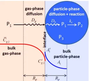
Figure 1.Schematic of the gas-particle mass-transfer process, with both diffusion and reaction occurring inside the particle phase.

actual particle-phase reactions that are important for SOA formation. In Sect. 4, we apply the model to evaluate the timescale of SOA partitioning and the associated evolution of the number and composition size distributions for a range of solute volatilities, bulk diffusivities, and particle-phase re-action rates. We close with a summary of our findings and their implications.

2 Dynamics of diffusion and reaction within a particle Consider an organic soluteithat diffuses from the gas phase to a single spherical organic aerosol particle and reacts irre-versibly with a pseudo-first-order rate constant kc (s−1)as

it diffuses inside the particle. This process is illustrated in Fig. 1 using three species (P1, P2, and P3) for simplicity.

The organic solute P1 diffuses and reacts to form a

non-volatile species P2inside an organic particle (of radiusRp)

that is initially composed of a nonvolatile organic speciesP3.

The solute’s gas-phase concentrations far away from the par-ticle (i.e., in the bulk gas-phase) and just above the parti-cle surface areCgandCs_g(mol cm−3(air)), respectively. The solute’s particle-phase concentration just inside the particle surface and at any location in the bulk of the particle are de-noted as As and A (mol cm−3(particle)), respectively. The gas- and particle-phase diffusivities of the solute areDgand Db(cm2s−1), respectively.

In this section we shall focus on the dynamics of diffu-sion and reaction inside the particle. In order to derive the timescales relevant to this problem, the particle, initially free of the organic solute (i.e., at time t=0), is assumed to be exposed to a constant concentration just inside the particle surface, As_i, at all times t >0 (this assumption will be re-laxed in Sect. 3 where we will relate the temporally chang-ing gas-phase concentration of the solute to its particle-phase

concentration). Assuming that the diffusive flux of the solute into the particle follows Fick’s law, the transient partial dif-ferential equation describing the particle-phase concentration

Ai(r, t )as a function of radiusrand timetcan be written as

∂Ai(r, t )

∂t =Db,i

1

r2 ∂ ∂r

r2∂Ai(r, t ) ∂r

−kc,iAi(r, t ). (1)

The particle is assumed to be spherically symmetrical with respect to the concentration profiles of the organic solute in the particle at any given time, so the concentration gradient at the center of the particle (i.e.,r=0) is always zero. These assumptions give rise to the following initial and boundary conditions:

I.C.:Ai(r,0)=0, (2a)

B.C.1:Ai(Rp, t )=Asi, (2b)

B.C.2:∂Ai(0, t )

∂r =0. (2c)

Equation (1), with conditions (Eq. 2), can be analytically solved by first solving the pure diffusion problem in the ab-sence of reaction (Carslaw and Jaeger, 1959; Crank, 1975) and then extending the solution to the case of first-order chemical reaction using the method of Danckwerts (1951) to yield the solution

Ai(r,t )

As_i = Rp

r

sinh(qir/Rp) sinh(qi) + 2Rp

π r

∞ P

n=1

(−1)nnsin(nπ r/Rp)

(qi/π )2+n2 exp

−

kc,i+

n2_π2_D b,i R2 p t _{, (3)}

whereqiis a dimensionless diffusion–reaction parameter

de-fined as the ratio of the particle radiusRp to the so-called reacto-diffusive lengthp

Db,i/ kc,i (Pöschl et al., 2007):

qi=Rp

s kc,i

Db,i

. (4)

It should be noted that this solution assumes thatRpremains constant with time, so diffusion of additional material into the particle is relatively small (this assumption will also be relaxed in Sect. 3). It is also worth noting here that in glassy particles, the diffusion fronts of plasticzing agents (such as water) may move linearly inward, leading to a linear depen-dence onRpinstead ofR2pin Fickian diffusion (Zobrist et al.,

2011).

Now, the timescale for Fickian diffusion of the dissolved soluteiin the particle, τda, and the timescale for chemical

reaction,τc, (Seinfeld and Pandis, 2006) are defined as τda,i=

R_p2 π2_D b,i

, (5)

τc,i=

1

kc,i

The model described by these equations has been applied to investigate mass-transfer limitation to the rate of SO2

oxi-dation in cloud droplets (Schwartz and Freiberg, 1981; Shi and Seinfeld, 1991), for which the droplets typically exceed a 10 µm diameter, with the aqueous-phase diffusivity about 10−5cm2s−1. Here we apply this model to analyze the ef-fects of particle-phase reactions in organic particles of sizes ranging from∼10−3to 1 µm diameter, withDbvalues

rang-ing from<10−18to 10−5cm−2s−1(Renbaum-Wolff et al., 2013). Since the actual particle-phase reactions of various organic species and the associated rate constants are still not well defined, we use a pseudo-first-order reaction as a proxy and vary its rate constant kc over several orders of magni-tude (10−5–10−1s−1)to examine its effect on the dynamics of particle growth.

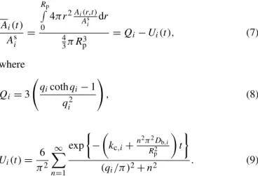
The right-hand side of Eq. (2) comprises two terms. The first term is the concentration profile at steady state with the surface concentration, while the second term describes the temporal evolution of the concentration profile. At steady state, the transient term disappears for t≫τdaandτc.

Fig-ure 2 illustrates the relative effects of bulk diffusivity and reaction rate constant on the temporal evolution of the diffus-ing solute concentration profiles within a particle of diameter

Dp=0.1 µm. The top row represents a liquid organic

parti-cle with a rather high bulk diffusivity, Db=10−6cm2s−1,

with (a) no reaction (kc=0), and (b) a modest reaction rate constant, kc=5×10−4s−1. In case (a), τda=2.5 µs, and the solute attains a uniform steady-state concentration pro-file across the particle radius in a little over 8 µs (i.e., about 4τda). The temporal evolution of the concentration profiles in case (b) appears to be identical to case (a) despite the presence of a chemical reaction, because τda is 2.5 µs but τc=2000 s, i.e., diffusion occurs much more rapidly than

re-action. In contrast, the bottom row represents a semisolid or-ganic particle,Db=10−15cm2s−1, with (c) no reaction, and

(d)kc=5×10−4s−1. In case (c),τda=2533 s (i.e., 42 min)

and∼160 min is required for the solute to attain a uniform steady-state profile. In case (d),τdaandτc are comparable,

and as a result the solute not only reaches the steady state sooner (in about 60 min) than in the no-reaction case, but also the steady-state concentration profile is visibly nonuni-form. This is a result of the fact that there is sufficient time for appreciable amounts of the solute to be consumed by the reaction as it diffuses towards the center of the particle.

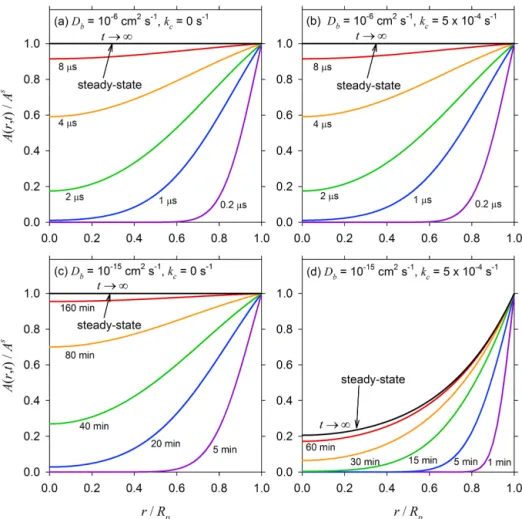
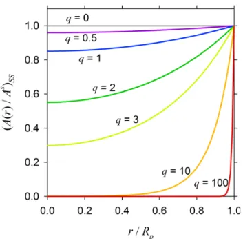
Figure 3 illustrates the steady-state concentration profiles for a range ofkc values (from 10−5to 0.1 s−1)in a particle

of diameterDp=0.1 µm with four different Dbvalues: (a)

10−6cm2s−1, (b) 10−12cm2s−1, (c) 10−13cm2s−1, and (d) 10−15cm2s−1. Altogether, these cases represent twenty dif-ferent combinations of τda andτc. In case (a), τda≪τcfor

all thekc values considered here, and as a result the

steady-state concentration profiles are essentially uniform across the entire particle, with the consumption of the solute by chemi-cal reaction occurring uniformly across the entire volume of the particle. In case (b), even though the particle is

consid-ered to be a semisolid withDb=10−12cm−2s−1,τda and τcbecome comparable only whenkc=0.1 s−1(and higher).

However, slower reactions produce nonuniform steady-state concentration profiles in cases (c) and (d) forDb values of

10−13cm2s−1and lower. In these cases, most of the solute is consumed near the surface of the particle, with a contration that becomes progressively depleted towards the cen-ter of the particle askc increases. Thus, the particle growth

is volume-reaction controlled when the concentration profile is uniform and tends to be surface-reaction controlled at the other extreme.

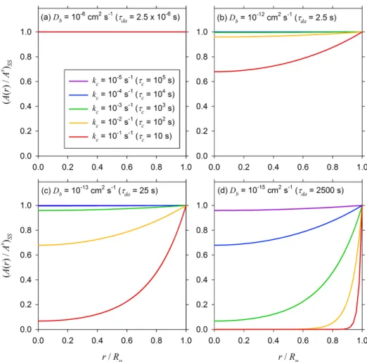
Since the timescale for diffusion varies asR_p2, the diffu-sion limitation to reaction also depends strongly on particle size. As shown in Fig. 4, the relative effects of particle size, bulk diffusivity, and reaction rate on the shape of the steady-state concentration profiles are concisely captured in terms of the dimensionless parameterq, which is a function ofRp, kc, and Db(Eq. 3). At low values ofq (<0.5), the

steady-state concentration profile is nearly uniform, but becomes in-creasingly nonuniform forqvalues on the order of unity and greater.

While the temporal evolution of the radial concentration profile is highly informative, the timescale to reach steady state, as well as the shape of the steady-state profile, can be conveniently quantified in terms of the average particle-phase concentration A(t ). We integrate the concentration profile given by Eq. (3) over the volume of the particle to obtain

Ai(t )

As_i =

Rp

R

0

4π r2Ai(r,t )

As_i dr

4 3π Rp3

=Qi−Ui(t ), (7)

where

Qi =3

qicothqi−1

q_i2 !

, (8)

Ui(t )=

6 π2 ∞ X n=1 exp −

kc,i+ n2_π2_D

b,i R2 p t

(qi/π )2+n2

. (9)

Here,Qiis the ratio of the average particle-phase

concentra-tion to the surface concentraconcentra-tion at steady state, whileUi(t )

is the transient term, the value of which is always equal toQi

att=0 and decreases exponentially to zero ast→ ∞. As noted earlier, the surface concentrationAs_i is assumed to be constant in the analytical solution of Eq. (1). However, since

As_ican gradually change over time due to changes in the gas-phase concentration and particle composition, it is more ap-propriate to refer to the steady state as quasi-steady state. The timescale to reach a quasi-steady state (τQSS) within the

Figure 2. Normalized transient concentration(A(r, t )/As)profiles as a function of normalized radius (r/Rp) for a particle of diameter

Rp=0.05 µm for different values of bulk-phase diffusivity and first-order reaction rate constants:(a)Db=10−6cm2s−1,kc=0 s−1;(b)

D_b=10−6cm2s−1,kc=5×10−4s−1;(c)Db=10−15cm2s−1,kc=0 s−1; and(d)Db=10−15cm2s−1,kc=5×10−4s−1.

quasi-steady-state termQi. Thus, settingUi(τQSS)=Qi/e,

we get

∞ X

n=1

exp

−

kc,i+n

2_π2_D b,i

R2 p

τQSS

(qi/π )2+n2

(10)

=1

e×

π2

2

qicothqi−1

q_i2 !

.

For a given set of values forDp,Db, andkc, Eq. (10) can be numerically solved forτQSSwith the bisection method.

We first examine the dependence of τQSS and Qon Db

andkcfor a particle ofDp=0.1 µm (Fig. 5). The values of Db are varied over 14 orders of magnitude from 10−19

(al-most solid) to 10−5cm2s−1(liquid water) to cover the full range of semisolid and liquid organic particles; andkc

val-ues are varied over 6 orders of magnitude from of 10−6(very slow reaction) to 1 s−1 (practically instantaneous reaction). As seen in Fig. 5a, the contours ofτQSSrange from 1 µs for

liquid particles to 1 day for highly viscous semisolid parti-cles. For the semisolid particles, there are two regions in the

semisolid zone as depicted by the gray dotted line. In the re-gion above the dotted line,τQSSis sensitive only to the value

ofkcand decreases rapidly with increase inkc. For instance,

at Db=10−19cm2s−1, τSS≈1 day for kc=5×10−6s−1 but decreases to<1 min forkc=10−2s−1. In the region be-low the dotted line, τQSS is sensitive only to the value of

Dbfor both semisolid and liquid particles. For example, at

Db≈10−14cm2s−1, τQSS remains constant at∼1 min for

kc values from 10−6 up to about 10−2s−1 (i.e., up to the dotted line) and only then becomes sensitive to reaction at higher values ofkc.τQSSis sensitive to bothkcandDbonly

in the relatively narrow envelope along the dotted line itself. As seen in Fig. 5b, the values ofQare<0.001 for highly viscous semisolid particles and highkc values, while they

approach unity asDbincreases andkc decreases. Note that

the dotted line in Fig. 5a roughly corresponds to the contour forQ=0.6 in Fig. 5b.

Next, we examine the dependence of τQSS and Q on

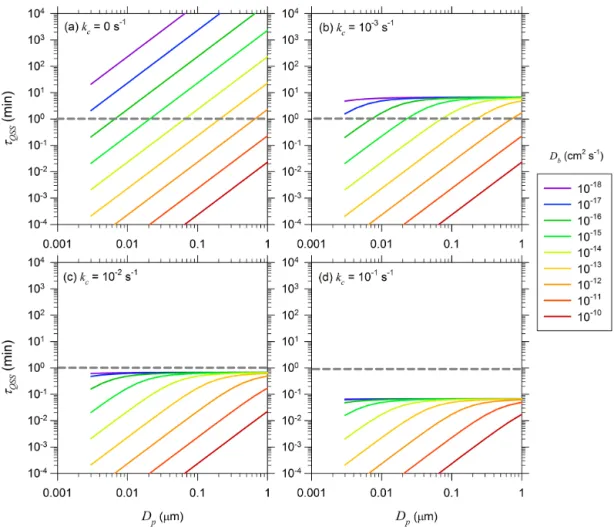
particle size. Figure 6 shows τQSS vs. Dp for Db values ranging from 10−18 to 10−10cm2s1 for (a) kc=0 s−1, (b)

Figure 3.Normalized steady-state concentration(A(r)/As)SSprofiles as a function ofr/Rpfor a particle of diameterRp=0.05 µm and a

range ofkcvalues for(a)Db=10−6cm2s−1,(b)Db=10−12cm2s−1,(c)Db=10−13cm2s−1, and(d)Db=10−15cm2s−1.

seen in Fig. 6a, for any given Db, τQSS increases by five

orders of magnitude as Dp increases from 0.003 to 1 µm.

At the upper end, particles with Db <10−18cm2s−1 have

a τQSS of about 10 min at Dp=0.003 µm and increase to

more than 104min atDp=0.1 µm. In contrast, particles with

Db>10−12cm2s−1 have τQSS below 1 min (indicated by the dotted gray line) for sizes up to 0.7 µm. From a practi-cal standpoint, since most ambient SOA particles are smaller than∼0.7 µm, concentration profiles of nonreacting solutes inside particles with Db>10−12cm2s−1 may be assumed to be at steady-state. However, significant diffusion limita-tion can exist for nonreacting solutes in particles with Db <10−12cm2s−1 depending on their size. In stark contrast, for reacting solutes,τQSSasymptotically approaches a

com-mon maximum value for all values of Db as the particle

size increases as shown in Fig. 6b, c, and d. This maximum value of τQSS is about 7, 0.7, and 0.07 min for kc=10−3,

10−2, and 0.1 s−1, respectively. The typical timescale for changes in the bulk gas-phase concentrations due to trans-port and chemical reaction is on the order 10 min or more. Thus, from a practical standpoint, the particle-phase concen-tration profiles of solutes reacting with kc>10−2s−1 (for

whichτQSS≤0.7 min) may be assumed to be at quasi-steady

state in particles of any size and anyDbvalue.

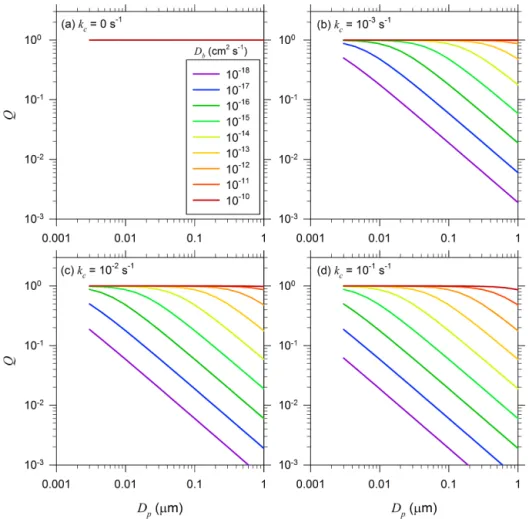
Figure 7 illustrates variation of Qwith Dp for the four

cases shown in Fig. 6. At quasi-steady state, the particle-phase concentration profile for nonreacting solutes is always uniform (i.e., Q=1) even though τQSS can differ signifi-cantly depending on the particle size andDbvalue (Fig. 7a). For reacting solutes withkcup to 0.1 s−1,Qremains nearly equal to unity in particles withDb>10−10cm2s−1andDp

up to 1 µm. ForDb<10−10cm2s−1,Qdecreases asDp in-creases for a givenDb, while it increases asDbincreases for

a givenDp.

In general, the above analysis indicates that (a) for a givenDp, a more reactive solute will reach quasi-steady state

sooner and exhibit a more nonuniform concentration profile than a less reactive one, especially in particles with lower

Dbthan higher, and (b) for a given set of values forkc and Db, a solute in smaller particles will reach quasi-steady state

Figure 4.Normalized(A(r)/As)_SSprofiles as a function ofr/Rp

for different values of the dimensionless diffuso-reactive parameter q.

3 Kinetic gas-particle partitioning model

We shall now describe the development of a new frame-work for modeling kinetic partitioning of SOA based on the insights gained from timescale analysis of the diffusion– reaction process within the particle phase. The framework takes into account solute volatility, gas-phase diffusion, in-terfacial mass accommodation, particle-phase diffusion, and particle-phase reaction. However, instead of numerically re-solving the concentration gradient inside the particle (Shi-raiwa et al., 2012a), which is computationally expensive and therefore impractical for inclusion in 3-D Eulerian models, we use the analytical expressions of the quasi-steady state and transient behavior of the solute diffusing and reacting within the particle.

3.1 Model framework

3.1.1 Single particle equations

We begin by relating the average particle-phase concentra-tion of the soluteAi(mol cm−3(particle)) to its average bulk

gas-phase concentrationCg,i (mol cm−3(air)) over a single

particle. Similar to the timescale for diffusion in the parti-cle phase (Eq. 5), the timescale for the gas-phase concentra-tion gradient outside the particle to reach a quasi-steady state (τdg)is given by Seinfeld and Pandis (2006):

τdg,i=

R2_p π2_Dg

,i

, (11)

whereDg,i (cm2s−1)is the gas-phase diffusivity. For a

typ-icalDg,i of 0.05 cm2s−1, the value ofτdg is on the order

10−8s or less for submicron-size aerosols, which is much smaller than the typical timescale for changes in the bulk gas-phase concentration in the ambient atmosphere. We can therefore safely assume that the gas-phase concentration pro-file of the solute around the particle is at quasi-steady state at any instant.

An ordinary differential equation describing the rate of change of Ai due to mass transfer between gas and a

sin-gle particle with particle-phase reaction can then be written as

dAi

dt =

3

Rpkg,i

Cg,i−Cgs,i

−kc,iAi, (12)

whereC_gs_,i(mol cm−3(air)) is the gas-phase concentration of the solute just outside the surface of the particle, and kg,i

(cm s−1)is the gas-side mass-transfer coefficient given as

kg,i=

Dg,i

Rp f (Kni, αi). (13)

Here f (Kni, αi) is the transition regime correction factor

(Fuchs and Sutugin, 1971) to the Maxwellian flux as a func-tion of the Knudsen numberKni=λi/Rp(where λi is the

mean free path) and the so-called mass accommodation co-efficient,αi, which is defined as the fraction (0≤αi≤1)of

the incoming molecules that is incorporated into the particle surface:

f (Kni, αi)=

0.75αi(1+Kni)

Kni(1+Kni)+0.283αiKni+0.75αi

. (14) While the above correction factor was derived from a numer-ical solution of the Boltzmann diffusion equation for neu-tron transfer to a black sphere (i.e., representative of light molecules in a heavy background gas), its applicability for higher-molecular-weight trace gases in air has been exper-imentally confirmed (Seinfeld and Pandis, 2006, and refer-ences therein).

The timescale to achieve interfacial phase equilibrium be-tweenC_gs_,i and the particle-phase concentration ofijust in-side the surface,As_i (mol cm−3(particle)), is at least (Seinfeld and Pandis, 2006)

τp,i=Db,i

4

αivi

2

, (15)

where vi is the average speed of solute molecules in the

gas phase. From kinetic theory of gasesvi=(8ℜT /π Mi)1/2

where ℜ is the universal gas constant (8.314×107 erg K−1mol−1),T (K)is temperature, andMi is the

molec-ular weight of the solute. For representative values ofDb,i≤

10−5cm2s−1,Mi=100 g mol−1,T =298 K, andαiranging

Figure 5. (a)Contour plots of:(a)particle-phase quasi-steady-state timescale (τQSS), and(b)quasi-steady-state parameterQ=(A/As)QSS

as functions of first-order rate constant (kc)and bulk diffusion coefficient (Db)for a species diffusing and reacting within semisolid and

liquid particles of diameterDp=0.1 µm.

Figure 6. Dependence of τQSS on particle diameter Dp for Db values ranging from 10−10 to 10−18cm2s−1: (a) kc=0 s−1, (b)

Figure 7.Dependence ofQon particle diameterDpforDbvalues ranging from 10−10to 10−18cm2s−1:(a)kc=0 s−1,(b)kc=10−3s−1, (c)kc=10−2s−1, and(d)kc=10−1s−1.

less, which means it can be safely assumed that the interfa-cial phase equilibrium is achieved virtually instantaneously. We thus relateC_gs_,i andAs_i according to Raoult’s law as

C_gs_,i= A s

i

P

j

As_jC ∗

g,i, (16)

where C_g∗_,i is the effective saturation vapor concentration (mol cm−3(air)), andP

jAsj is the total particle-phase

con-centration of all the organic species at the surface. However, since the surface concentrations of all the species are not al-ways known, we use the total average particle-phase concen-trationP

jAjas an approximation forPjAsj. Thus Eq. (12)

is rewritten in terms ofAs_i as

dAi

dt =

3

Rpkg,i 

 Cg,i−

As_i P

j

Aj

C_g∗_,i 



−kc,iAi. (17)

As_i can be assumed to be equal to Ai in liquid particles for

a nonreactive or slowly reacting solute that quickly attains a

uniform concentration profile (as was previously shown in Fig. 2a, b). But, as discussed in the previous section, this equality may not hold for reactive and nonreactive solutes in semisolid particles. In such cases, Eq. (7) can be used to expressAs_i in terms of Ai as long as As_i does not change

with time, because the analytical solution to Eq. (1) assumes a constantAs_i according to the boundary condition (Eq. 2b). In practice, however, Eq. (7) can be used if the timescale for changes in As_i are much greater than the timescale for the solute to relax to its quasi-steady-state profile inside the par-ticle. With this caveat, we get

dAi

dt =

3

Rp

kg,i

( Cg,i−

Ai

P

jAj

C∗_g,i

(Qi−Ui(t ))

)

−kc,iAi. (18)

Note that Eq. (18) describes kinetic mass transfer of speciesi

mass-transfer during SOA partitioning (Bowman et al.,1997; Saathoff et al., 2009; Parikh et al., 2011). However, αdoes not correctly capture the mass-transfer limitations due to dif-fusion and chemical reaction occurring within the bulk of the particle. In the present framework, the interfacial and bulk particle-phase limitations to mass transfer are represented separately, with the appropriate dependence for the latter on particle size.

In Eq. (18), the termUi(t )is to be evaluated at the “time

since start”. Equation (18) can therefore only be used in a La-grangian box model framework for a “closed system” where we can specify an initial concentration of the solute vapor (at time t=0), which then partitions to the particle phase as a function of time. The solute vapor in the closed system is not subjected to emissions, dilution, and loss due to gas-phase oxidation. In the case of no particle-gas-phase reaction, the solute vapor will eventually reach equilibrium with the par-ticles. In the presence of particle-phase reaction, the solute vapor concentration will eventually decay to zero. This is in stark contrast with the “general system” such as the ambient atmosphere and 3-D atmospheric chemistry transport models where the solute vapor at a given location may continuously change due to emissions, dilution, and gas-phase chemistry in addition to gas-particle partitioning. As a result, it is not possible to evaluateUi(t )in the general system, because we

cannot keep track of the “time since start” in the same sense as used in the transient analytical solution to Eq. (1). There-fore, based on the value ofkcand the associated timescale for the particle-phase concentration profile to reach quasi-steady state (τQSS), the following two approximations to Eq. (18) are made for it to be applicable to the general system. Approximation 1: for fast reactions (kc,i≥0.01 s−1) As discussed in the previous section (Fig. 6c),τQSSfor a

so-lute reacting withkc,i≥0.01 s−1is less than 1 min in

parti-cles with any Db and of any size. Compared to the typical

time step values of 5 min or greater in 3-D Eulerian mod-els, the particle-phase concentration profile for solutes with

τQSS≤1min may be assumed to be at quasi-steady state, and the termUi(t )can be safely neglected in Eq. (17) to yield

dAi

dt =

3

Rpkg,i (

Cg,i−

Ai

P

jAj

C_g∗_,i Qi

)

−kc,iAi (19)

forkc,i≥0.01 s−1.

A similar equation was derived by Shi and Seinfeld (1991) for reactive mass transport of SO2 (with Henry’s law for

absorption) in cloud droplets assuming quasi-steady state within the droplet phase. Now, askc→0,Q→1, and mass

transfer is governed entirely by gas-phase diffusion and inter-facial mass accommodation in Eq. (19). As a result, Eq. (19) tends to lose its ability to capture the resistance to mass trans-fer due to slow diffusion in the particle phase as kc→0.

Therefore, an alternate treatment for mass transfer is needed for slow reactions.

Approximation 2: for slow reactions (kc,i<0.01 s−1) For kc,i<0.01 s−1 (or τQSS>1 min), we use the

classi-cal two-film theory of mass transfer between the gas and particle phases. The two-film theory was originally intro-duced by Lewis and Whitman (1924) and has been widely used to model mass transfer in two phase systems, with and without chemical reactions (Astarita, 1967; Doraiswamy and Sharma, 1984; Bird et al., 2007). Figure 8 shows the schematic of the two-film model, which assumes that the concentration gradients in the gas and particle phases are confined in the respective hypothetical “films” adjacent to the interface. The gas- and particle-side film thicknesses are denoted by δg and δp (cm), respectively, and the

respec-tive mass-transfer coefficients (cm s−1)are defined askg= Dg/δg andkp=Db/δp. The overall gas-side mass-transfer

coefficientKg(cm s−1)is then given by (see Appendix A for

the derivation) 1 Kg,i = 1 kg,i + 1 kp,i

C_g∗_,i P

jAj

!

. (20)

The ordinary differential equation describing the rate of change ofAi due to gas-particle mass-transfer and

particle-phase reaction can then be written in terms of the overall driving force as

dAi

dt =

3

RpKg,i (

Cg,i−

Ai

P

jAj

C∗_g,i )

−kc,iAi (21)

forkc,i<0.01 s−1.

A similar equation was derived by Zaveri (1997) for reactive mass transport of SO2(with Henry’s law for absorption) in

cloud droplets assuming quasi-steady state within the droplet phase. The advantage of the two-film model formulation is that the diffusion limitations from both the gas and particle sides are represented in the overall mass-transfer coefficient, and can therefore be used to model mass transfer of slow-reacting solutes. The gas-side mass-transfer coefficient (kg)

is already known from Eq. (13) whereδg=Rp. However, the

particle-side film thickness,δp, and thereforekp, are not

read-ily known. In a general system, the bulk gas- and particle-phase concentrations of a reactive semivolatile solute tend to reach a quasi-steady state when the net source rate of the so-lute in the gas phase is relatively steady. Since both Eqs. (19) and (21) describe the same process, they should predict iden-tical gas- and particle-phase concentrations at quasi-steady-state. Thus, settingdAi/dt=0 in both Eqs. (19) and (21)

and equating the expressions forAi/Cg,iresulting from each

of them yields the general expressions forδpandkpin terms

ofDb,kc, andRp(see Appendix B for the derivation): δp,i=Rp

1−Qi

qicothqi−1

kp,i=

Db,i

Rp _q

icothqi−1

1−Qi

. (23)

For the limiting case of a nonreactive solute,kc→0,q→0, Q→1 and Eq. (23) reduces to

kp,i=5

Db,i

Rp

. (24)

3.1.2 Polydisperse aerosol equations

We now extend the closed system box model Eq. (18) for a single particle to a polydisperse aerosol in a sectional frame-work. For a given size-section m, with number concentra-tionNm(cm−3(air)) and particle radiusRp,m(cm), we define

Ca,i,m(mol cm−3(air)) as the total average concentration of

soluteiin size-sectionm:

Ca,i,m=

4 3π R

3

p,mNmAi,m. (25)

Multiplying Eq. (18) by(4π R_p3_,mNm/3)yields: dCa,i,m

dt =4π R

2

p,mNmkg,i,m

Cg,i−Ca,i,m

Si,m

(Qi−Ui(t ))

−kc,iCa,i,m,(26)

whereSi,mis the saturation ratio:

Si,m=

C∗_g,i P

jCa,j,m

. (27)

The corresponding equation governing the gas-phase con-centration of soluteiis

dCg,i dt = −

X

m

4π Rp2,mNmkg,i,m

Cg,i−Ca,i,m

Si,m

(Qi−Ui(t ))

. (28) Similarly, the particle-phase and gas-phase equations for polydisperse aerosols in the general system are as follows. Approximation 1: forkc,i≥0.01 s−1

dCa,i,m

dt =4π R 2

p,mNmkg,i,m

Cg,i−Ca,i,m Si,m

Qi

−kc,iCa,i,m, (29)

dCg,i

dt = − X

m

4π R2_p,mNmkg,i,m

Cg,i−Ca,i,m Si,m

Qi

. (30)

Approximation 2: forkc,i<0.01 s−1 dCa,i,m

dt =4π R

2

p,mNmKg,i,m Cg,i−Ca,i,mSi,m−kc,iCa,i,m, (31)

dCg,i

dt = − X

m

h

4π R_p2_,mNmKg,i,m Cg,i−Ca,i,mSi,m

i . (32)

Figure 8.Schematic of the two-film theory.

The proposed framework, described by Eqs. (29) through (32), is relatively simple and amenable for use in regional and global aerosol models, although it presently awaits spec-ification of the actual particle-phase chemical reactions that are important for SOA formation.

We have implemented both the closed system and general system frameworks in the computationally efficient, multi-component aerosol box-model MOSAIC and adapted the ex-isting semiimplicit Euler method solver to numerically inte-grate the set of coupled ordinary differential equations for any number of solutes i over any number of size bins m

(Zaveri et al., 2008). Sectional growth in MOSAIC is cal-culated using the two-moment approach of Simmel and Wur-zler (2006). The closed system framework is to be used in the box-model version only while the general system framework can be used in both box and 3-D Eulerian models. The com-plete solution to these equations may be labeled as “seminu-merical” because the particle-phase diffusion–reaction pro-cess is represented analytically while the set of ordinary dif-ferential equations themselves are integrated numerically.

MOSAIC already performs kinetic partitioning of in-organic gases (H2SO4, HNO3, HCl, and NH3) to

Figure 9.Comparison of MOSAIC (lines) and finite-difference model (filled circles) solutions for gas-phase concentration decay in a closed system due to kinetic gas-particle partitioning to particles with initialDp=0.2 µm,N=5000 cm−3,Db=10−15cm2s−1andkcranging

from 0 to 0.1 s−1for three solute volatilities:(a)C∗_g=10 µg m−3,(b)C_g∗=100 µg m−3, and(c)C_g∗=1000 µg m−3.

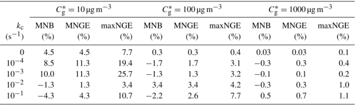
Table 1.Bias and error statistics for MOSAIC predictions for the closed system simulations.

C_g∗=10 µg m−3 C∗_g=100 µg m−3 C_g∗=1000 µg m−3 kc MNB MNGE maxNGE MNB MNGE maxNGE MNB MNGE maxNGE

(s−1) (%) (%) (%) (%) (%) (%) (%) (%) (%) 0 4.5 4.5 7.7 0.3 0.3 0.4 0.03 0.03 0.1 10−4 8.5 11.3 19.4 −1.7 1.7 3.1 −0.3 0.3 0.4 10−3 10.0 11.3 25.7 −1.3 1.3 3.2 −0.1 0.1 0.2 10−2 −1.3 1.3 3.4 3.4 3.4 4.2 −0.3 0.3 1.0 10−1 −4.3 4.3 10.7 −2.2 2.6 7.7 0.5 0.7 1.1

3.2 Model validation

We shall now validate the new framework in MOSAIC against a “fully numerical” finite-difference solution to Eq. (1) with a flux-type boundary condition that includes mass transfer of the solute between the gas phase and the par-ticle surface. The volume of the spherical parpar-ticle is resolved with multiple layers, and diffusion and reaction of the solute species through these layers are integrated numerically. We used 300 uniformly spaced layers in the present exercise. The finite-difference model is conceptually similar to the

KM-GAP model (Shiraiwa et al., 2012a), but does not include re-versible adsorption at the surface and heat transfer processes. The finite-difference solution is used as a benchmark here because it rigorously solves Eq. (1) and does not assume the surface concentration to remain constant with time.

For validation purposes, we consider a monodisperse semisolid aerosol composed of nonvolatile organic species

P3 (molecular weight 100 g mol−1 and density 1 g cm−3), with initial particle diameter Dp=0.2 µm, particle num-ber concentration N=5000 cm−3, and bulk diffusivity

and density of the condensing solute (P1) and its reaction

product species (P2)are also assumed to be 100 g mol−1and

1 g cm−3, respectively. The three species (P1,P2, andP3)are

assumed to form an ideal solution that participates in the ab-sorption ofP1according to Raoult’s law. Model validation is

demonstrated below for both closed and general systems. 3.2.1 Closed system

In three separate closed system cases, the initial monodis-perse aerosol was exposed to the solute (P1) gas con-centration of 2 µg m−3 with volatility C_g∗=10, 100, and 1000 µg m−3. Figure 9 compares the solution given by MO-SAIC (Eqs. 26, 28) with the finite-difference model solution for gas-phase concentration decay due to kinetic gas-particle partitioning for particle-phase reaction rate constantskc rang-ing from 0 to 0.1 s−1. Whenkc=0, the gas-phase concentra-tion reaches an equilibrium value that depends on the solute volatility, while in other cases it decays to zero at different rates as governed by the particle-phase reaction rate constant and diffusion limitation. MOSAIC is able to reproduce the finite-difference results quite well, although small deviations can be seen during the initial portions of the gas decay for

kc≤10−4s−1andCg∗=10 and 100 µg m−3. The following

metrics were used to quantify the accuracy of MOSAIC rel-ative to the finite-difference (FD) model:

Mean normalized bias,MNB=CMOSAIC_g,1 −C_gFD_,1/CFD_g,1, (33)

Mean normalized gross error,MNGE= C

MOSAIC g,1 −CFDg,1

/C

FD g,1, (34)

Maximum normalized gross error,maxNGE (35) =max

C MOSAIC g,1 −C

FD g,1 /C

FD g,1

.

These metrics were calculated using the model outputs at 5 min intervals for the 10 h-long simulations. However, neg-ligibly small gas-phase concentrations (<0.05 µg m−3₎

to-wards the latter part of the simulations (where applicable) were excluded in the calculations of the metrics. The results are displayed in Table 1. The MNB and MNGE are com-parable in magnitude and range from∼0.1 to∼10 %, with values greater than∼5 % seen only forC_g∗=10 µg m−3. The large maxNGE values (>20 %) seen forC∗

g=10 µg m−3

oc-cur as the gas-phase concentrations approach zero. Overall, the agreement between the two models is quite good for the closed system.

3.2.2 General system

In three separate general system cases, the initial monodis-perse aerosol was exposed to soluteP1withC_g∗=10, 100, and 1000 µg m−3 at a constant gas-phase source rate of

γ=0.1 µg m−3h−1in each case. The initial gas-phase con-centration ofP1was zero in each case. Figure 10 compares

the evolution of the gas-phase concentration ofP1predicted

by MOSAIC (Eqs. 29–32) and the finite-difference model. The particle-phase reaction rate constant kc ranged from 0

to 0.1 s−1. Whenkc =0, the gas-phase concentration ofP1

increases almost linearly with time upon reaching quasi-equilibrium with the particle phase. Forkc>0, the gas-phase

concentration ofP1 remains constant after the initial build

up as the source rate is balanced by the loss rate due to particle-phase diffusion and reaction. This quasi-steady-state gas-phase concentration level depends on the combination of

C_g∗,Db, and kc. For C_g∗=10 µg m−3, the time required to establish quasi-steady state between gas and particle phases ranges from less than 1 h atkc=0.1 s−1 _{to more than 20 h}

atkc=10−4s−1. The time to reach quasi-equilibrium (for

nonreactive solutes) and quasi-steady state (for reactive so-lutes) increases as the value ofC∗

g increases.

Approxima-tions 1 and 2 in MOSAIC are able to capture both the initial “spin-up” phase, when the gas-phase concentration builds up, as well as the later phase where the concentration remains in quasi-equilibrium or quasi-steady state. Furthermore, for

kc=10−3s−1, approximation 1 (black dotted line in Fig. 10)

yields nearly identical results as approximation 2 for all three

C_g∗values, indicating that the transition from one to the other does not cause a sudden change in the behavior of the so-lution. Approximation 1 predicts faster gas uptake than the finite-difference model for slow reactions while approxima-tion 2 predicts slower gas uptake than the finite-difference model for fast reactions (not shown), especially for low-volatility solutes (C∗

g= ∼10 µg m−3). A combination of

ap-proximations 1 and 2 is thus needed to cover the full range of possiblekcvalues.

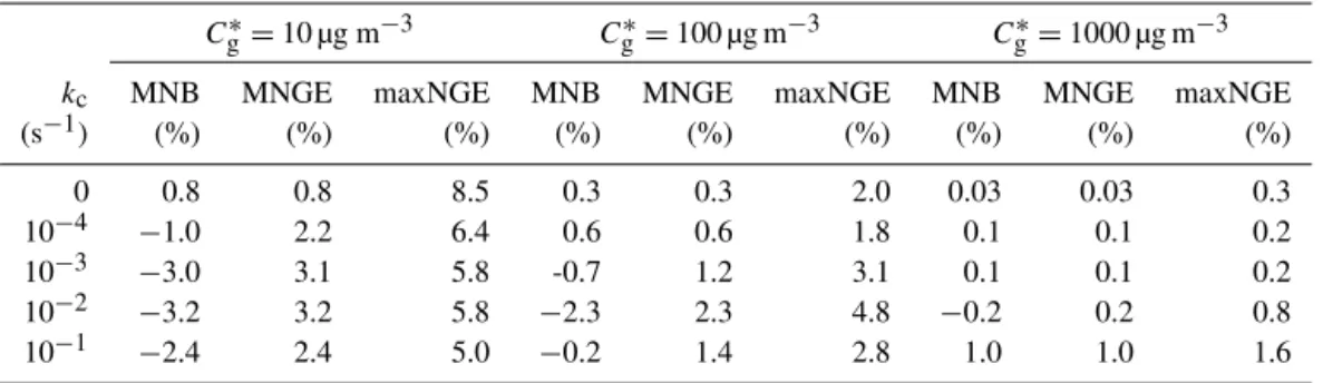
The normalized gross errors in MOSAIC are relatively large during the spin-up phase where the gas-phase concen-trations are very small. In a 3-D Eulerian model applica-tion, the spin-up phase occurs at the beginning of the simu-lation and is usually discarded. Here, we discard the first two hours of spin-up in each simulation to avoid small gas-phase concentrations when calculating the bias and error metrics, shown in Table 2. Both MNB and MNGE are generally less than∼3 %. The maxNGE values ranged between 0.3 and 8.5 %. The overall performance of MOSAIC for the general system is excellent.

3.3 Future considerations

Figure 10. Comparison of MOSAIC (lines) and finite-difference model (filled circles) solutions for gas-phase concentration evolution in a general system due to kinetic gas-particle partitioning to particles with initialDp=0.2 µm,N=5000 cm−3, Db=10−15cm2s−1,

γ=0.1 µg m−3h−1, andkc ranging from 0 to 0.1 s−1 for three solute volatilities:(a)C∗g=10 µg m−3, (b)Cg∗=100 µg m−3, and(c)

C_g∗=1000 µg m−3.

Table 2.Bias and error statistics for MOSAIC predictions for the general system simulations.

C_g∗=10 µg m−3 C∗_g=100 µg m−3 C_g∗=1000 µg m−3 kc MNB MNGE maxNGE MNB MNGE maxNGE MNB MNGE maxNGE

(s−1) (%) (%) (%) (%) (%) (%) (%) (%) (%) 0 0.8 0.8 8.5 0.3 0.3 2.0 0.03 0.03 0.3 10−4 −1.0 2.2 6.4 0.6 0.6 1.8 0.1 0.1 0.2 10−3 −3.0 3.1 5.8 -0.7 1.2 3.1 0.1 0.1 0.2 10−2 −3.2 3.2 5.8 −2.3 2.3 4.8 −0.2 0.2 0.8 10−1 −2.4 2.4 5.0 −0.2 1.4 2.8 1.0 1.0 1.6

First, the present framework uses a pseudo-first order (PFO) reaction for a condensing solute as a proxy for second-order chemical reactions that may occur within a particle. The assumption of a PFO reaction for the condensing solute is valid when the preexisting bulk reactant species is uni-formly distributed with the depth of the particle, e.g., when the reaction timescale for the reactant species is much longer than that for diffusion. The issue arises when the reaction timescale is much shorter than that for diffusion such that the bulk reactant species is not homogeneously distributed

depth-wise (Berkemeier et al., 2013). In such cases, it may be possible to parameterize the PFO reaction rate constant for the condensing solute in terms of its second order rate con-stant multiplied by the volume average concentration of the preexisting reactant solutes in the particle phase. The detailed finite-difference model using second order reactions can be used to provide guidance for improving and validating the parameterized reactions in the seminumerical framework.

diffu-sivities, it cannot explicitly treat the potential variation of dif-fusivity within a given particle of complex morphology. Ex-amples include black carbon or solid ammonium sulfate par-ticles coated with organics as well as parpar-ticles with nonideal internal mixtures of hydrophobic and hydrophilic organics. The diffusion–reaction process inside such complex and po-tentially nonspherical particles will again have to be param-eterized based on the average bulk properties, with possible guidance from more detailed finite-difference models where applicable.

Third, as mentioned earlier, the new framework can be readily adapted to kinetically partition water soluble organic gases into the particulate aqueous phase if that is the only liq-uid phase in the particle. However, additional work is needed to extend the present framework to mixed inorganic–organic particles in which water and organics may form separate liq-uid phases (You et al., 2012).

4 Results and discussion

We now apply the updated MOSAIC model to a series of polydisperse aerosol scenarios to investigate the influence of particle-phase reactions, phase state, and solute volatility on SOA partitioning timescale and the evolution of aerosol size distribution. While the exact mechanism(s) responsible for the growth of newly formed particles (1–10 nm range) is still unknown, it is suspected to occur via effectively irreversible condensation of very-low-volatility organic species that can overcome the strong Kelvin effect (Pierce et al., 2011). In the present study, we focus on the competitive growth dynamics of the Aitken and accumulation mode particles, as might re-sult after the newly formed particles have grown up to Aitken mode sizes. The Kelvin effect and coagulation are neglected for simplicity. Figure 11 shows the initial aerosol number and volume size distributions used for this exercise. Again, this preexisting aerosol is assumed to be composed of nonvolatile organic species (P3)of molecular weight 100 g mol−1 and

density 1 g cm−3. The entire size distribution, consisting of an Aitken mode and an accumulation mode, is discretized over 1000 logarithmically spaced size bins (lower boundary of the smallest bin=0.008 µm and the upper boundary of the largest bin=1 µm). The total number concentration of parti-cles in the Aitken mode is 6223 cm−3 while that in the ac-cumulation mode is 1139 cm−3_{; the total aerosol mass}

con-centration is 2 µg m−3. Figure 11 also shows the condensa-tional sinkkCS,i,m=4π Rp2,mNmkg,i,mfor each size binmas

a function ofDp. For this particular size distribution, the sum

of kCSover all the size bins in the Aitken mode is equal to

that in the accumulation mode, so that there is no initial bias in the condensation rate of the solute species towards either mode merely due to differences in the initial condensational sink rates for the two modes. Both closed and general sys-tems scenarios are examined.

Figure 11.Initial aerosol number and volume size distributions along with the condensational sinkkCS. The dashed line

demar-cates the Aitken mode from the accumulation mode and the initial condensation sink is such that the sum ofkCSover all the size bins

in the Aitken mode is equal to that in the accumulation mode.

4.1 Closed system

A set of closed system simulations was performed in which the initial organic aerosol was separately exposed to the so-lute gas (P1)with three different C∗g values: 10, 100, and

1000 µg m−3(molecular weight=100 g mol−1), with an ini-tial gas-phase concentration of 6 µg m−3 in each case. For each solute volatility case, the effect of aerosol-phase state was examined using four differentDbvalues: 10−6, 10−12,

10−13, and 10−15cm2s−1. In all cases,kcwas set at 0.01 s−1

so thatτSSwas always less than∼0.7 min across the entire

size distribution. In each case, the simulation was run until the gas-phase solute was completely absorbed and reacted to form a nonvolatile product in the particle phase. Again, the molecular weight and density of the product species (P2)

were assumed to be 100 g mol−1and 1 g cm−3, respectively, and all three species (P1,P2, andP3)were assumed to form an ideal solution that participated in the absorption of P1

according to Raoult’s law. An additional set of reference simulations were performed for two extreme scenarios: (1) instantaneous particle-phase reaction (i.e.,kc→ ∞), which is equivalent to solving the nonvolatile solute condensation case (i.e., mechanism #1), and (2) no particle-phase reac-tion (kc=0), which is referred to as Raoult’s law partitioning

Figure 12. Results for the instantaneous reaction reference case (kc→ ∞; equivalent to nonvolatile solute condensation):(a)

gas-phase concentration decay, (b)temporal evolution of aerosol size distribution, and (c) temporal evolution of the mass fraction of newly formed SOA.

4.1.1 Reference cases

We shall first discuss the results of the closed system ref-erence cases. Figure 12 shows the gas-phase decay and the corresponding temporal evolution of aerosol size distribu-tion and mass fracdistribu-tion of newly formed SOA for the in-stantaneous particle-phase reaction case. Here, gas-particle partitioning is independent of the particle-phase state and is governed entirely by gas-phase diffusion limitation. Va-por concentration is completely depleted in about 1 h, and

aerosol size distribution evolution displays the well-known narrowing characteristics as the small particles grow faster (more precisely, have greater d lnDp/dt ) than the large

ones (Zhang et al., 2012). Consequently, the mass frac-tion of the newly formed SOA in smaller particles is much higher than in the larger ones. Note that in the SOA mass fraction panel, the left-most point on each line with mass fraction ≈1 corresponds to the smallest initial particles (Dp=0.008 µm att=0).

In contrast, aerosol evolution due to Raoult’s law parti-tioning depends on both solute volatility and particle-phase state. Figure 13 shows the gas-phase concentration decay and the corresponding aerosol size distribution and SOA mass fraction evolution for the less volatile solute with

C_g∗=10 µg m−3_{. The effect of phase state is illustrated with}

two bulk diffusivities:Db=10−6and 10−15cm2s−1. In the case with liquid particles (Db=10−6_cm2_s−1_{)there is}

neg-ligible resistance to mass transfer within the particle (refer to Fig. 6a), and as a result the vapor concentration rapidly de-creases during the first 1 h and reaches a steady state in about 7.5 h. In the first∼20 min, the size distribution exhibits the narrowing of the Aitken mode similar to that seen in gas-phase diffusion-limited growth, although not as intense. The SOA mass fraction reaches up to 0.97 in small particles while it is only about 0.25 in the large particles. However, as the vapor concentration decreases further, the peak of the size distribution begins to decrease and the width broadens due to evaporation from small particles while the large particles continue to grow (Zhang et al., 2012). The SOA mass frac-tion in small particles decreases to 0.75, while it gradually in-creases to 0.75 in the large particles. The vapor concentration remains steady while this interparticle mass transfer (via the gas phase) occurs over a relatively longer period (∼480 h) until the entire aerosol size distribution reaches equilibrium. Similar behavior is seen in the case with semisolid par-ticles (Db=10−15cm2s−1), although the timescale over

which it occurs is relatively longer due to much higher particle-phase diffusion limitation. While the vapor concen-tration declines rapidly in the beginning (e-folding timescale of 16.5 h), it takes about 175 h to reach the steady state and more than 400 h for the aerosol size distribution to reach equilibrium. Also, because the particle-phase diffusion limi-tation is much less in small particles than the large ones (refer to Fig. 6a), the Aitken mode exhibits more intense narrowing and a higher peak (at about 1 h) than seen in liquid particles. Then, again, as the vapor concentration decreases further, the width broadens and the peak decreases due to evaporation of small particles while the large ones continue to grow more slowly. The final aerosol size distribution and SOA mass fraction across the size spectrum are identical (within numer-ical errors) to those obtained in the liquid-particle case.

Figure 13.Results for kinetic SOA partitioning due to Raoult’s law (kc=0 s−1)forCg∗=10 µg m−3:(a)gas-phase concentration decay

forDb=10−6and 10−15cm2s−1,(b)aerosol evolution forDb=10−6cm2s−1,(c)SOA mass fraction evolution forDb=10−6cm2s−1, (d)aerosol evolution forDb=10−15cm2s−1, and(e)SOA mass fraction evolution forDb=10−15cm2s−1. In both cases, the final (i.e.,

equilibrium) concentration of the newly formed SOA is 6 µg m−3.

steady state in just 20 min (vs. 7.5 h for C∗

g=10 µg m−3)

while it takes nearly 400 h (vs. 175 h for C∗

g=10 µg m−3)

in the case with semisolid particles (Db=10−15_cm2_s−1_).

Again, the final aerosol size distribution and SOA mass frac-tion solufrac-tions at equilibrium are identical to those obtained for theC∗

g=10 µg m−3cases, but their temporal evolutions

are quite different. In the case with liquid particles, the width of the aerosol size distribution does not narrow and the peak height remains the same as the particles grow. This is be-cause the small particles quickly attain a quasi-equilibrium state with the more volatile solute. Consequently, the SOA mass fraction in the small particles quickly reaches the equi-librium value of 0.75 (instead of overshooting as seen for

C_g∗=10 µg m−3)while the larger particles catch up slightly

more slowly. The entire size distribution reaches equilibrium within 1 h.

In the case with semisolid particles, the Aitken mode size distribution narrows (similar to that seen in Fig. 13a) in the first few minutes, but broadens back within 30 min. Again, the SOA mass fraction in small particles quickly reaches the equilibrium value of 0.75, while it still takes∼480 h for the large particles in the spectrum to reach equilibrium due to the significant diffusion limitation in the particle phase.

4.1.2 Reactive partitioning cases

We now present results for the closed-system reactive parti-tioning cases withkc=0.01 s−1. Fig. 15 shows vapor

Figure 14.Same as Fig. 13, exceptC_g∗=1000 µg m−3.

10−6_{to 10}−15_cm2_s−1_{. It also shows a plot of the e-folding}

timescale (τg)for the decay as a function ofDbfor the

dif-ferent volatilities. Each plot includes the reference case of in-stantaneous reaction for comparison. Unlike in Raoult’s law partitioning, the vapor concentration always decays to zero in reactive partitioning and the decay rate slows down with in-crease inC_g∗. The vapor decay rate also slows down with de-crease inDband it is especially sensitive toDbin semisolid

particles.

Figure 16 illustrates the effects of the differentC_g∗andDb

values on the final aerosol size distribution. The final results for the reference cases of instantaneous reaction and Raoult’s law partitioning are also shown for easy comparison. In the case of C_g∗=10 µg m−3, the Aitken mode exhibits signifi-cant narrowing for all values ofDb. The narrowing becomes more pronounced for Db <10−13cm2s−1 with the shape of the entire size distribution forDb=10−15cm2s−1being

nearly identical to that for the instantaneous reaction

refer-ence case. Further decrease inDb will produce even more narrowing. Since there is negligible particle-phase diffusion limitation forDb>10−10cm2s−1(Q≈1; Fig. 7c), the size

distribution of liquid aerosol narrows because its initial evo-lution (in the case of low volatility solutes) resembles that of gas-phase diffusion-limited growth, and the particle-phase reaction rate is fast enough to transform the absorbed so-lute to a nonvolatile product before it can evaporate. ForDb <10−13cm2s−1, the steep gradient inQacross the size dis-tribution results in significantly lower surface concentrations over small semisolid particles compared to the large ones. The small semisolid particles therefore grow even faster than the large ones compared to the corresponding liquid aerosol case, causing relatively more intense narrowing of the size distribution.

Figure 15.Gas-phase concentration decay due to kinetic SOA partitioning with particle-phase reaction (kc=0.01 s−1)for bulk diffusivities

ranging from 10−6to 10−15cm2s−1and three gas volatilities:(a)C_g∗=10 µg m−3,(b)C_g∗=100 µg m−3, and(c)C_g∗=1000 µg m−3. Each plot also shows gas-phase concentration decay for the reference case of instantaneous reaction (black line,kc→ ∞). In each case, the final

concentration of the newly formed SOA is 6 µg m−3. Panel(d)shows the plot of gas-phase concentration decay timescale (τg)as a function

ofDbfor the different gas volatilities.

a result, the final size distributions forDb≤10−12cm2s−1 progressively resemble that of the Raoult’s law partition-ing case. However, significant narrowpartition-ing is still seen for

Db=10−15cm2s−1due to the steep gradient inQacross the

size distribution, which causes the small semisolid particles to grow much faster than the large semisolid ones when com-pared to the corresponding liquid aerosol case whereQ≈1 across the entire size distribution. In general, the final size distribution shape tends to be closer to that for instantaneous reaction case for lowerC_g∗andDbvalues and higherkc

val-ues, while it tends to be closer to that for Raoult’s law parti-tioning for higherC_g∗andDband lowerkc.

Figure 17 illustrates the influence of C_g∗ and Db values on the final SOA mass fraction size distribution. Curves for the two reference cases are also included for comparison. In the case ofC_g∗=10 µg m−3, the curves for allDbvalues are similar to that of the instantaneous reference case due to appreciable narrowing of the size distribution. But asC∗ g

increases, the SOA mass fraction curves progressively be-come more uniform for Db=10−6 cm2s−1 while they

re-main nonuniform forDb<10−12cm2s−1for particles with Dp>0.2 µ m. In allCg∗cases, the SOA mass fraction curves

for Db=10−15cm2s−1 closely resemble the instantaneous

reaction case.

4.2 General system

A set of general system simulations was performed in which the initial organic aerosol was separately exposed to solutes withC_g∗=10, 100, and 1000 µg m−3at a moderate but con-stant gas-phase source rate of γ=0.6 µg m−3h−1 in each case. The effect of aerosol-phase state was examined using two differentDbvalues: 10−6and 10−15cm2s−1. For each combination ofC_g∗andDbvalues, the effect of particle-phase reaction was examined forkc=0.01, 0.1, 1, and∞s−1. Each simulation was 12 h long.

Figure 18 shows the time evolutions of total SOA mass concentration for liquid particles (Db=10−6cm2s−1)

with different solute C∗

g values and the corresponding

fi-nal aerosol size distributions at t=12 h. In the case with

C_g∗=10 µg m−3, the SOA formation rate is essentially the same for kc≥0.01 s−1, with a total of about 7 µg m−3

SOA formed at the end of 12 h. Appreciable narrowing of the Aitken mode size distribution occurs forkc=0.01 s−1,

which is qualitatively similar to the closed system results for

Db=10−6cm2s−1shown previously in Fig. 16a. Higherkc

so-Figure 16. Initial (dashed line) and final (solid lines) aerosol number size distribution due to Raoult’s law gas-particle partitioning cou-pled with particle-phase reaction (kc=0.01 s−1)for bulk diffusivities ranging from 10−6to 10−15cm2s−1and three gas volatilities:(a)

C_g∗=10 µg m−3,(b)C_g∗=100 µg m−3, and(c)C_g∗=1000 µg m−3. Panel(d)shows the final size distributions for the two reference cases: instantaneous reaction (black line;kc→ ∞)and Raoult’s law partitioning (gray line;kc=0) for anyDbandCg∗>0. As illustrated in Fig. 15,

the time required to reach the final state differs significantly for different cases, but the final SOA formed in each case is 6 µg m−3.

lute vapor tends towards quasi-equilibrium with the parti-cle phase for lowkc values. As a result, the SOA formation

rate slows down and the Aitken mode shapes for kc=0.01

s−1 qualitatively tend to resemble that of Raoult’s law par-titioning in the closed system shown previously in Fig. 16b, c. But as kc increases, the mass transfer becomes progres-sively more gas-phase-diffusion limited, which results in faster growth of the smaller particles and, therefore, increas-ing narrowincreas-ing of the Aitken mode.

Figure 19 shows the results for semisolid particles (Db=10−15cm2s−1). It is seen that the presence of signifi-cant particle-phase diffusion limitation slows down the SOA formation rates, especially with increasingC∗

g and

decreas-ingkc. The marked size-dependence of the diffusion

limita-tion also gives rise to more intense narrowing of the size dis-tribution than seen in the corresponding liquid-particle cases. In the absence of a particle-phase reaction (i.e.,kc=0, not

shown in the figures) only∼1.2 µg m−3of SOA is formed in both the liquid and semisolid aerosol cases after 12 h when

C_g∗=10 µg m−3while negligibly small amounts of SOA are formed for higherC_g∗values. Overall, the growth character-istics seen in the general system cases considered here are qualitatively similar to the closed system results, although significant differences between them can occur if the

va-por source rate is appreciably different than the one used in the present study. For instance, if the vapor source rate is very small, then the growth characteristics will tend towards Raoult’s law partitioning. In contrast, if the vapor source rate is very high, then the growth will tend to become gas-phase diffusion limited.

5 Summary and implications

We have extended the computationally efficient MOSAIC aerosol model (Zaveri et al., 2008) to include a new frame-work for kinetic SOA partitioning that takes into account so-lute volatility, gas-phase diffusion, interfacial mass accom-modation, particle-phase diffusion, and particle-phase reac-tion. The framework uses a combination of (a) an analytical quasi-steady-state treatment for the diffusion–reaction pro-cess within the particle phase for fast-reacting organic solutes such that the timescales (τQSS)for their particle-phase

Figure 17. Final size distributions of the newly formed SOA mass fraction for different Db values and (a) Cg∗=10 µg m−3, (b)

C_g∗=100 µg m−3, and(c)C_g∗=1000 µg m−3. Each panel also shows the reference plots for instantaneous reaction (black line;kc→ ∞)

and for Raoult’s law partitioning (gray line;kc=0 s−1)for anyDbandCg∗>0.

the new framework can be readily adapted to kinetically par-tition water soluble organic gases into the particulate aque-ous phase if that is the only liquid phase in the particle. Ad-ditional work is needed to treat mass transfer of gas-phase species to mixed inorganic–organic particles that experience liquid–liquid phase separation (You et al., 2012). The pro-posed framework is amenable for use in regional and global atmospheric models, although it currently awaits specifica-tion of the various gas- and particle-phase chemistries and the related physicochemical properties that are important for SOA formation.

In the present study, we have applied the model to evaluate the effects of solute volatility (C_g∗), particle-phase bulk dif-fusivity (Db), and particle-phase chemical reaction, as

exem-plified by the pseudo-first-order rate constant (kc), on kinetic

SOA partitioning. We focus on the competitive growth dy-namics of the Aitken and accumulation mode particles due to condensation while the Kelvin effect and coagulation are ne-glected for simplicity. Our analysis shows that the timescale of SOA partitioning and the associated evolution of aerosol number and composition size distributions depend on the complex interplay between C_g∗,Db, and kc, each of which can vary over several orders of magnitude. The key findings and their implications are summarized below.

1. In the case of instantaneous particle-phase reaction

Figure 18. Temporal evolution of total SOA mass concentration (left column) and aerosol size distribution (right column) at t=12 h forDb=10−6cm2s−1, γ=0.6 µg m−3h−1, kc=0.01 to ∞s−1, and three different solute volatilities:(a, b)Cg∗=10 µg m−3, (c, d)

C_g∗=100 µg m−3, and(e, f)C_g∗=1000 µg m−3.

gas-phase concentration is appreciably higher than the solute vapor volatility. Also, while the vapor concen-tration may reach a steady-state relatively quickly, the timescale for the “narrowed” aerosol size distribution to relax back to its final (equilibrium) shape can be on the order of a few minutes to days, depending on the values ofDbandCg∗.

3. In the case of reactive partitioning (finitekc; mechanism

#3), the size distribution experiences permanent narrow-ing (Shiraiwa et al., 2013a), which can be especially

pronounced for low values of C_g∗ (∼10 µg m−3 and less) andDb (<10−13cm2s−1)and high values ofkc

(∼0.01 s−1and higher). AsC_g∗andDbincrease andkc

decreases, the narrowing reduces and the final size dis-tribution tends to resemble that produced by mechanism #2. But unlike in mechanism #2, the gas-phase concen-tration of the solute eventually decays to zero and the partitioning timescale increases with increase inC∗

gand

decrease inDbandkc. The partitioning timescale and

sensi-Figure 19.Same as Fig. 18, exceptD_b=10−15cm2s−1.

tive to the phase state whenDbis about 10−13cm2s−1

or less. At Db=10−15cm2s−1 andkc=0.01 s−1, the

decay timescale ranges from 1 h for C_g∗=10 µg m−3 to about 3 days for C_g∗=1000 µg m−3. Consequently, for intermediate volatility solutes (C_g∗ >1000 µg m−3)

to partition in appreciable amounts to semisolid SOA via particle-phase reactions, theirkc values need to be >0.1 s−1.

4. From a practical standpoint, the particle-phase concen-tration profiles of a solute (with anyC_g∗) reacting with

kc >0.01 s−1 may be assumed to be at steady-state in

particles of any size and any phase state. Furthermore, forkc≤0.1 s−1andDb≥10−10cm2s−1, the

particle-phase reaction occurs uniformly through the entire vol-ume of submicron particles. At higherkcor lower Db

dependence on the particle-phase state, together control the SOA partitioning timescale and the size distribution evolution.

5. Observations of the evolution of the size distribution can provide valuable clues about the underlying mecha-nisms of SOA formation (Riipinen et al., 2011; Shiraiwa et al., 2013a). However, all three mechanisms, under certain combinations ofC_g∗,Db, andkcvalues, can

pro-duce similar-looking aerosol number size distributions. A concerted experimental strategy is therefore neces-sary to properly constrain these and other key model parameters and effectively evaluate the next generation of SOA models that treat phase-state thermodynamics, particle-phase diffusion and particle-phase reactions.

6. A proper representation of these physicochemical pro-cesses and parameters is needed to reliably predict not only the total SOA mass, but also its composition-and number-diameter distributions, which together de-termine the overall optical and cloud-nucleating proper-ties.