Numerical uncertainty at mesoscale in a Lagrangian model in complex terrain

(1)

www.geosci-model-dev.net/5/1127/2012/ doi:10.5194/gmd-5-1127-2012

Geoscientific

Model Development

Numerical uncertainty at mesoscale in a Lagrangian model in

complex terrain

J. Brioude1,2, W. M. Angevine1,2, S. A. McKeen1,2, and E.-Y. Hsie1,2

1_{Cooperative Institute for Research in Environmental Sciences, University of Colorado at Boulder, Boulder, Colorado, USA} 2_{Chemical Sciences Division, Earth System Research Laboratory, NOAA, Boulder, Colorado, USA}

Correspondence to:J. Brioude (jerome.brioude@noaa.gov)

Received: 13 April 2012 – Published in Geosci. Model Dev. Discuss.: 27 April 2012 Revised: 24 August 2012 – Accepted: 24 August 2012 – Published: 17 September 2012

Abstract.Recently, it has been shown that mass conserva-tion in Lagrangian models is improved by using time-average winds out of Eulerian models. In this study, we evaluate the mass conservation and trajectory uncertainties in com-plex terrain at mesoscale using the FLEXPART Lagrangian particle dispersion model coupled with the WRF mesoscale model. The specific form of vertical wind used is found to have a large effect. Time average wind with time aver-age sigma dot (σ˙), instantaneous wind with geometric carte-sian vertical wind (w) and instantaneous wind with σ˙ are used to simulate mixing ratios of a passive tracer in for-ward and backfor-ward runs using different time interval outputs and horizontal resolutions in California. Mass conservation in the FLEXPART model was not an issue when using time-average wind or instantaneous wind withσ˙. However, mass was poorly conserved using instantaneous wind withw, with a typical variation of 25 % within 24 h.

Uncertainties in surface residence time (a backtrajectory product commonly used in source receptor studies or in-verse modeling) calculated for each backtrajectory run were also analyzed. The smallest uncertainties were systematically found when using time-average wind. Uncertainties using in-stantaneous wind withσ˙ were slightly larger, as long as the time interval of output was sufficiently small. The largest un-certainties were found when using instantaneous wind with w. Those uncertainties were found to be linearly correlated with the local average gradient of orography. Differences in uncertainty were much smaller when trajectories were calcu-lated over flat terrain. For a typical run at mesoscale in com-plex terrain, 4 km horizontal resolution and 1 h time interval output, the average uncertainty and bias in surface residence time is, respectively, 8.4 % and−2.5 % using time-average

wind, and 13 % and−3.7 % using instantaneous wind with

˙

σ in complex terrain. The corresponding values for instanta-neous wind with cartesianwwere 24 % and−11 %.

While the use of time-average wind systematically im-proves uncertainty in FLEXPART, the improvements are small, and therfore a systematic use of time-average wind in Lagrangian models is not necessarily required. Use of carte-sian vertical wind in complex terrain, however, should be avoided.

1 Introduction

(2)

However, Lagrangian models suffer from numerical uncer-tainties due to interpolation in space and time of simulated meteorological fields, and errors due to the conversion from the native vertical coordinate of the Eulerian model onto the vertical coordinate used in the Lagrangian model. Further-more, mass conservation could be an issue when the vertical velocity is not mass balanced with horizontal winds.

Recently, Nehrkorn et al. (2010) analyzed the mass con-servation in a Lagrangian model using instantaneous or time-average wind from a mesoscale Eulerian model. They used mass weighted time average wind (horizontal and vertical) and instantaneous wind for driving the STILT Lagrangian model using the Weather Research and Forecast (WRF) Eu-lerian forecast model at a horizontal resolution of 12×_{12 km}2 and a time resolution of 1 h. They found that the mass conser-vation using instantaneous wind from WRF was very poor, and using time average wind was “crucial in improving the mass conservation properties of the coupled modeling sys-tem”. The authors suggested that those large differences in mass conservation were due to the fact that mass weighted time average winds were less subject to errors in interpola-tions and vertical coordinate transformainterpola-tions than instanta-neous winds.

Grell et al. (2004) have shown that wind variability can be captured by instantaneous winds, as long as the output time interval is short enough for a given horizontal resolu-tion. For instance, a 3-km horizontal resolution run would need an output interval of 15 min to capture 50 % of the wind variability in the case of a cold front passage. Therefore, it is important to understand how trajectory uncertainties and mass conservation vary with horizontal resolution and out-put interval when using instantaneous wind or time-average wind. Theoretically, the mass conservation should be iden-tical when using time-average wind or instantaneous wind when a very short output interval is used, the lower limit be-ing the time step within the Eulerian model. Furthermore, vertical coordinate transformation between the native Eule-rian model coordinate and the Lagrangian model coordinate can be responsible for additional uncertainties. One can ex-pect larger uncertainties in Lagrangian trajectories in com-plex terrain where errors in vertical coordinate transforma-tion are the largest.

In this article, we present an analysis of mass conservation and trajectory uncertainties using time-average and instanta-neous winds for different output time intervals, vertical ve-locity variables, and horizontal grid spacing. The Lagrangian trajectories were calculated by a modified version of the FLEXPART Lagrangian particle dispersion model with WRF output using (1) the instantaneous wind with cartesian verti-cal velocity, (2) the instantaneous wind with sigma dotas ver-tical velocity, and (3) mass weighted time averaged horizon-tal and vertical winds. Our goal is to evaluate the impact of those different types of wind on the uncertainties of trajectory calculations that could reduce the accuracy of typical appli-cations of Lagrangian particle dispersion model runs, such as

source receptor relationships for inverse modeling or mixing ratio estimates of a tracer. We do not evaluate the accuracy of the wind and meteorological fields from the Eulerian model itself in this paper.

Section 2 presents in detail the WRF and FLEXPART model configurations. Section 3 presents results on wind di-vergence, mass conservation and uncertainties. A discussion and conclusion is given in Sect. 4.

2 Models 2.1 WRF

We used a configuration of the Weather Research and Fore-casting (WRF) mesoscale research model version 3.3 that uses mass weighted variables (ARW core) with nested grids at 36, 12 and 4 km horizontal spacing with 60 vertical levels. The model was initialized at 12:00 UTC and run for 36 h each day. The model was initialized with ERA-interim reanalysis (Simmons et al., 2007). The MYJ planetary boundary layer (PBL) scheme and Noah land surface scheme were used. Other significant physics options were Eta-Ferrier micro-physics, RRTM-G (Rapid Radiative Transfer Model) long-wave and Dudhia shortlong-wave radiation. and Grell-Devenyi cu-mulus (outer domain only).

Angevine et al. (2012) present detailed evaluations of this simulation (their run EM4N). It should be noted that the fi-delity of the simulated winds to reality does not influence the results presented here.

The WRF output is on a Arakawa C-grid with terrain fol-lowing pressure based sigma levels (called eta levels in Ska-marock et al., 2008). It includes instantaneous horizontal wind on sigma levels (variable names U andV in m s−1), a geometric cartesian vertical velocity (W in m s−1) that we call w, an instantaneous sigma dot vertical velocity (WW in s−1) that we call σ˙, and mass weighted time-average winds on sigma levels (AVGFLX RUM, AVGFLX RVM, AVGFLX WWM). The time-average vertical wind is a mass weighted time average sigma dot, and therefore its vertical coordinate transformation in FLEXPART is equivalent to the one applied onσ˙.

The 4 km and 12 km grid spacing domains, and 30 min, 1 h and 2 h time interval outputs are used to run FLEXPART. 2.2 FLEXPART

(3)

values of a Lagrangian timescale, vertical velocity and mix-ing height (see Eq. 19 in Stohl et al., 2005). An upper limit was fixed at 180 s for horizontal mixing and 36 s for vertical mixing. On average, the time scale was 100 s for horizontal mixing and 20 s for vertical mixing. The horizontal resolu-tion of the FLEXPART output domain was 8×8 km2.

The Hanna turbulent scheme (Hanna, 1982) was used to represent turbulent mixing in the boundary layer1. Param-eters used in the Hanna scheme are calculated internally by FLEXPART (e.g., PBL mixing height, friction velocity, etc.) rather than retrieved directly from the WRF model out-put to improve consistency with the wind fields. See Stohl et al. (2005) for further details.

We chose California for our analysis. Gradients in orog-raphy in this region can be particularly strong. The CAL-NEX campaign took place in California in 2010, with sev-eral flights dedicated to characterizing surface emissions in Central Valley and the Los Angeles basin. California is a dif-ficult region to simulate due to complex terrain, differences in surface moisture between Central Valley and Los Angeles Basin, sea breeze, etc. See Angevine et al. (2012) for further details.

To examine mass consistency, we compared forward and backward trajectories. Forward trajectories were simulated over 24 h. Each trajectory carried an equal mass of a passive tracer based on an arbitrary homogeneous surface flux. Over-all, 15 million trajectories were released homogeneously over the surface domain, and continuously from May 16th to May 20th 2010. Mixing ratios of this tracer were output every hour within grid cells with a horizontal resolution of 8×8 km2and within 14 vertical layers stretched between the surface and 4 km in altitude.

Backward trajectories were calculated 4 times a day be-tween 17 and 19 May over 24 h from 108 different geograph-ical locations (every 5 grid cells in x direction, and every 10 grid cells in y direction) and at 3 different vertical levels (between 0 and 100 m, between 200 and 400 m and between 800 and 1100 m) that match grid cell positions in the forward run output domain. 5000 particles are released for each time and location. For each set of trajectories, the output consists of a residence time in the surface layer weighted by the atmo-spheric density (the so-called footprint). When this output is combined with a surface flux, one can calculate a mixing ra-tio for each set of backtrajectories (e.g., Brioude et al., 2011). We used the same surface flux of the homogeneous tracer used in the forward run to calculate a mixing ratio at each starting location of the backtrajectories.

Lin et al. (2003) have shown that asymmetry between backward and forward runs arise mostly from errors in the mass balance of the driving winds. In our case, perfectly

1_{To date, an option that uses 3-D fields of Turbulent Kinetic}

En-ergy is also available in the FLEXPART-WRF version. However, the well mixed criterion is not satisfied using this option, and is therefore not recommended at the time of submission.

mass balanced winds would give the same mixing ratio at each location from either forward or backward experiments, assuming that the Hanna turbulent scheme satisfy the well mixed criterion. Overall, 3888 mixing ratios are calculated for each experiment. In Sect. 3, we present differences using different wind treatments, different grid spacing (4 km and 12 km) and different time interval outputs (30 min, 1 h and 2 h).

3 Mass conservation and uncertainties 3.1 Wind divergence

According to Skamarock et al. (2008), the mass in the WRF model is fully conserved relative to the sixth-order Runge-Kutta advection algorithm. Therefore, horizontal and verti-cal winds in the WRF outputs are considered mass conserva-tive. Loss of mass conservation in a Lagrangian model should arise from unit conversion, vertical coordinate transforma-tion and uncertainties in the turbulent scheme used. Mass conservation in FLEXPART can be calculated for each grid cell using the mass continuity equation based on the wind divergence in cartesian coordinate.

1 ρ

∂ρ ∂t =

1 ρ

_∂ρu

∂x + ∂ρv

∂y + ∂ρW

∂z

. (1)

Withu,v andW being the horizontal and vertical wind in cartesian terrain following coordinate in FLEXPART,ρ be-ing the air density. We calculated it after convertbe-ing the WRF wind on sigma coordinates onto the terrain following carte-sian vertical coordinate within FLEXPART. The gradients are calculated using a central finite difference method.

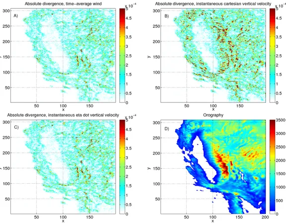
Figure 1 presents the evaluation of Eq. (1) for each grid cell at 50 m above ground on 16 May at 00z using mass weighted time average winds, instantaneous winds with cartesian geometric vertical velocity (w) and instantaneous winds with sigma dot (σ˙). The differences in divergence at 50 m are representative of the differences found within the PBL for other dates. The wind divergence is small and al-most identical when using time-average wind or instanta-neous winds withσ˙. Non-zero values come from uncertain-ties in converting the winds onto the FLEXPART vertical co-ordinate, or due to non-hydrostatic terms in the WRF model. The wind divergence is larger and more variable using the instantaneous wind with w, especially in complex terrain. However, no differences are found between wind divergences calculated by the three methods over flat terrain (either over the ocean or Central Valley). The strong divergence in com-plex terrain is the consequence of uncertainties inwrelated to variations in orography.

(4)

Fig. 1.Absolute wind divergence at about 50 m in altitude using(a)time-average wind,(b) instantaneous wind with cartesian vertical velocity, and(c)instantaneous wind with sigma dot (in s−1).(d)Orography (in m).

corrective factor is of the form:

W=w−u∂Z ∂x −v

∂Z

∂y, (2)

withZbeing the orography from WRF output, andW being the terrain following vertical velocity.

There are two possible reasons for the large differences in wind divergence usingwandσ˙. The first possibility is that wcannot be accurately converted into a vertical velocity on a terrain following cartesian coordinate within a Lagrangian model. For instance, the termsudZ/dx andvdZ/dy are un-derestimated within FLEXPART as they need to be calcu-lated over 2dx and 2dy. Within WRF, the horizontal grid is staggered. Uncertainties from coordinate transformation is much smaller when usingσ˙ (or the time-average equiv-alent) because it involves a conversion from a terrain follow-ing pressure based sigma coordinate (in WRF) onto a terrain following cartesian coordinate (in FLEXPART). In this case, a corrective factor involves only horizontal differences in geopotential between those 2 terrain following coordinates, and is very small in magnitude. This fact is valid for any of-fline Lagrangian model with a terrain following coordinate. This deficiency does not occur when using fully Lagrangian models.

A second reason might come from the fact that in the WRF model, the mass weightedwis a prognostic variable, while the mass weightedσ˙ is a diagnostic variable used in the mass continuity equation resolved by the model that involves mass weighteduandv. Sincewis a prognostic variable, it might have additional uncertainties due to uncertainties in the prog-nostic equation in steep terrain thatσ˙ might not have. It is also important to notice that the differences in wind diver-gence found with this particular configuration might be dif-ferent using other PBL schemes or using a stronger damping coefficient for acoustic waves. However, we are confident that usingσ˙ would systematically improve the wind diver-gence for any configuration.

Nehrkorn et al. (2010) compared mass weighted time av-erage wind on sigma levels with instantaneous wind using geometric cartesianwfrom the WRF output. Their analysis involves the same errors in vertical coordinate transforma-tions that have been explained above, which could have con-tributed to the differences they found on mass conservation.

(5)

30 min

4 km 1 hour 4 km 2 hours 4 km 30 min 12 km 1 hour 12 km 2 hours 12 km

0.4 0.6 0.8 1

slope

30 min

0 0.2 0.4 0.6 0.8 1

linear correlation

time average wind instantaneous cartesian w instantaneous sigma dot instantenous divergence based

Fig. 2.(Top) slope and (bottom) linear correlation of mixing ratio between forward and backward runs, for 6 different experiments using 4 types of winds. See Table 1 and Sect. 3.2 for details.

FLEXPART based on Eq. (1) assuming hydrostatic condi-tions, that we callWf.

In the following subsections, we show results of mass con-servation and uncertainty using time-average wind, and in-stantaneous wind usingw,σ˙ andWf.

3.2 Mass conservation

In this section, we present comparisons of mixing ratio of a passive tracer at different locations based on forward runs and backward runs calculated over 24 h. A perfectly mass conserving model should be reversible in time, in a sense that backward and forward trajectories should give the same results (Lin et al., 2003). A mass conserving model should therefore have identical mixing ratios based on forward and backward runs. A distribution of mixing ratios from forward and backward runs should have a slope of 1, and a linear cor-relation of 1. These tests involving mixing ratios are equiv-alent to the count of trajectories between backward and for-ward runs in Nehrkorn et al. (2010).

It is important to notice that a source of uncertainty beside transport and mixing in FLEXPART is the limited number of trajectories used in this study. We used 5000 trajectories per location in the backward runs, and 15 millions of trajec-tory in each forward runs. Uncertainties between backward and forward runs at each location could come from the lim-ited number of trajectories to calculate mixing ratios within each grid cells. However, it should only affect the linear

cor-relations between mixing ratios from backward and forward runs, and should not modify the slopes.

Figure 2 and Table 1 present the slopes and linear correla-tions calculated in complex terrain using the 4 different types of wind, and using 30 min, 1 h, or 2 h output interval and 4 km or 12 km horizontal grid. A slope lower than 1 means a loss of mass in backward runs or gain of mass in forward runs.

Using 30 min time interval output with 4 km resolution, the slopes from the runs that use mass weighted time aver-age wind and instantaneous wind withσ˙ are very close to 1 (0.996 and 1.001, respectively). It means that FLEXPART loses (or gains) less than 0.4 % and 0.1 % of mass within 24 h. Their linear correlations are the largest found (0.931 and 0.929) among the different experiments. On average, the slopes from the runs using time-average wind and instanta-neous wind withσ˙ are different by less than 2 %, except for the experiment using 12 km resolution and 2 h output (4 %). These results show that differences in mass conservation in FLEXPART between runs using mass weighted time average wind and instantaneous wind withσ˙ is insignificant.

(6)

Table 1.Mass conservation experiments (in complex terrain) using time-average (“mean”) wind, instantaneous wind with cartesian windw

from WRF (“cartesian”), instantaneous wind with sigma dot from WRF, and instantaneous wind with vertical wind calculated internally in FLEXPART, for 3 different output intervals and 2 WRF horizontal grid spacings.

4 km 12 km

Experiment Geometric slope Linear correlation Geometric slope Linear correlation

Mean 0.5 h 0.996 0.931 0.982 0.886

Cartesian 0.5 h 0.750 0.812 0.782 0.276

sigma dot 0.5 h 1.001 0.929 0.961 0.86

Internal 0.5 h 1.03 0.912 1.033 0.857

Mean 1 h 1.01 0.929 1.002 0.881

Cartesian 1 h 0.751 0.806 0.481 0.220

sigma dot 1 h 1.01 0.926 0.988 0.859

Internal 1 h 1.055 0.905 1.054 0.853

Mean 2 h 1.051 0.926 1.038 0.878

Cartesian 2 h 0.783 0.815 0.73 0.30

sigma dot 2 h 1.053 0.912 1.000 0.854

Internal 2 h 1.097 0.888 1.097 0.828

mixing ratios are poorly correlated using 12 km resolution (correlation less than 0.3).

Runs using instantaneous wind withWf are significantly

less mass conserving than using mass weighted time average wind or instantaneous wind withσ˙, but much better than us-ing cartesian vertical velocityw. For a typical time interval of 1 h, the slope is about 1.05, which means that the mass varies by 5 % within 24 h in the model.

The results found using instantaneous wind withw con-firm the results found in Nehrkorn et al. (2010). In com-plex terrain, the mass variation is about 25 % within 24 h, and therefore, the use of w should be avoided. However, we hardly see a benefit using time-average wind instead of instantaneous wind (using σ˙) in terms of mass conser-vation, and therefore disagree with the conclusions given by Nehrkorn et al. (2010) that time-average wind is cru-cial to have mass conservation within a Lagrangian model at mesoscale. Those results are in agrement with the conclu-sions found in Sect. 3.1.

3.3 Surface residence time uncertainties

In this section, trajectory uncertainties in each experiment are investigated by comparing the surface residence time found in each grid cell for each backward run. Those biases and un-certainties can be used to estimate, for instance, unun-certainties involved in source-receptor relationships.

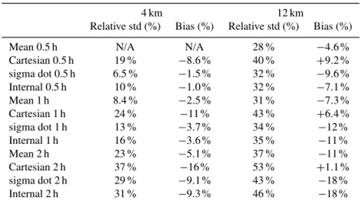
Figure 3 and Table 2 present relative standard devia-tion (%) and bias (%) for each experiment relatively to the best FLEXPART backward run, namely the run using mass weighted time average winds at 4 km resolution and 30 min output interval. The relative standard deviation is an estimate of the average uncertainty of residence time within each grid cell, and the relative bias is an estimate of the average dif-ference of surface residence time between each run and the reference run. The relative biases are the consequence of

dif-Table 2.Average relative error of the surface residence time in each grid cell relatively to the FLEXPART runs that use time-average wind at 4 km and 0.5 h time interval output.

4 km 12 km

Relative std (%) Bias (%) Relative std (%) Bias (%)

Mean 0.5 h N/A N/A 28 % −4.6 %

Cartesian 0.5 h 19 % −8.6 % 40 % +9.2 % sigma dot 0.5 h 6.5 % −₁_._{5 %} _{32 %} −₉_._{6 %}

Internal 0.5 h 10 % −1.0 % 32 % −7.1 % Mean 1 h 8.4 % −2.5 % 31 % −7.3 % Cartesian 1 h 24 % −11 % 43 % +6.4 % sigma dot 1 h 13 % −3.7 % 34 % −12 % Internal 1 h 16 % −3.6 % 35 % −11 % Mean 2 h 23 % −5.1 % 37 % −11 % Cartesian 2 h 37 % −16 % 53 % +1.1 % sigma dot 2 h 29 % −9.1 % 43 % −18 % Internal 2 h 31 % −9.3 % 46 % −18 %

ferences in vertical transport and differences in mass con-servation between each run and the reference run. Errors in vertical velocity impact mostly the bias, while errors in the horizontal wind impact the relative standard deviation.

(7)

30 min

0 20 40 60 80

relative standard deviation(%)

time average wind instantaneous cartesian w instantaneous sigma dot instantenous divergence based

30 min

−20 −10 0 10

relative bias (%)

Fig. 3.Relative standard deviation (top) and relative bias (bottom) for different experiments using footprints from the run at 30 min time interval output and 4 km horizontal resolution that uses time-average wind as reference. See Table 2 and Sect. 3.3 for details.

The most significant differences are found when using the 2 h time interval output. The bias using instantaneous wind is about 2 times larger than using time average wind.

The values of relative bias and uncertainty using instanta-neous wind withWf are equivalent to those usingσ˙.

The largest uncertainties and biases are found using the ge-ometric cartesian vertical velocityw. Uncertainty varies from 19 %–53 %, and relative bias varies from−16 % to+9.2 %. The relative bias becomes systematically positive when using 12 km resolution output. We did not investigate in detail the reason. For a typical output interval of 1 h, the relative stan-dard deviation is 24 % at 4 km resolution and 43 % at 12 km resolution, while the relative bias is−11 % and+6.4 %, re-spectively.

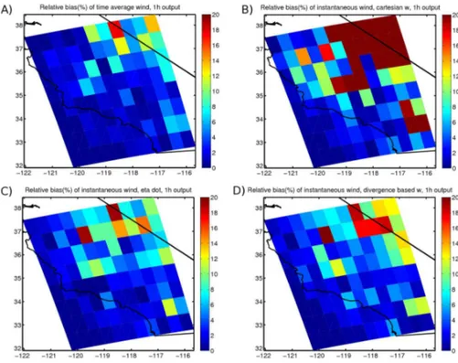
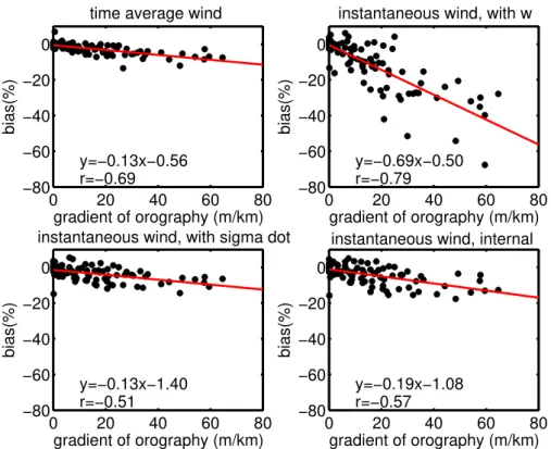
Figure 4 presents maps of relative biases at 1 h time inter-val output and 4 km resolution. Those plots are representative of the geographical distribution of biases using other time in-terval outputs and resolutions. As expected, the largest bias in each grid cell is found using instantaneous wind withw, and the smallest using time average winds. A gradient of bias is visible, directed from the ocean toward the continent for each run. It is not related to any boundary effect in the FLEXPART domain, but due to differences in orography. Therefore, re-sults found in Fig. 3 or Table 2 are valid for complex terrain, but are not necessarily applicable to domains with flat terrain. Figure 5 presents the relationship between relative biases and average gradient of orography calculated within 16 km of

each location with a time interval output of 1 h and 4 km res-olution. Figure 6 presents the relationship between relative standard deviation and average gradient of orography. Lin-ear relationships are correlated enough to fit a linLin-ear slope across.

For an average orographic gradient of 40 m km−1, typi-cally found near mountains, the bias is−5.7 % for time aver-age wind,−6.6 % for instantaneous wind withσ,˙ −8.7 % for instantaneous wind withWf and−28 % for instantaneous

wind with w (relative standard deviation of 7.5 %, 10 %, 15 % and 30 %, respectively). In flat terrain situation (orog-raphy gradient close to 0 m km−1_{), the biases only vary from}

−0.5 to−1.4 % among the 4 runs (relative standard deviation varying from 5 % to 10 %). Numerical uncertainties increase with orography because the gradient of orography becomes more uncertain and subgrid wind variability increases. It is also the reason why uncertainties in Table 2 increase with the resolution and time interval output.

(8)

Fig. 4.Maps of relative bias (%) using(a)time average wind,(b)instantaneous wind with cartesian vertical velocity,(c)instantaneous wind with sigma dot, and(d)instantaneous wind with divergence based vertical velocity with 1 h time interval output and 4×_{4 km resolution.}

4 Discussion and conclusion

We have shown differences in wind divergences when using the geometric cartesian vertical velocity with instantaneous wind (w) compared to using sigma dot(σ˙) or time average

˙

σ out of the WRF mesoscale model. No simple method can be used to correctly convert the geometric cartesian vertical velocity onto terrain following coordinates in complex ter-rain. As a result, wind is not mass balanced when usingw. As shown in Sect. 3.3, the mass within the model using in-stantaneous wind withwcan vary by 25 % within 24 h, and the residence time within grid cells can be uncertain by 19– 53 %, depending on the horizontal resolution or time interval output. However, in flat terrain, those uncertainties become much smaller and therefore the geometric cartesian vertical velocity with instantaneous wind can be used in Lagrangian models as long as the variation in orography within the do-main of interest stays small. Uncertainties in the inversion technique used in Brioude et al. (2011, 2012) in the Houston region by using instantaneous wind with geometric cartesian vertical velocity can be evaluated to about 10 %, smaller than typical uncertainties in PBL mixing height (about 20 %). Us-ing a wind divergence based vertical velocity (Wf), the mass

conservation and uncertainty improve compared tow, but is less accurate thanσ˙.Wf can be used as an alternative towif

no other options are available.

Mass conservation in the FLEXPART model was not an is-sue when using instantaneous wind withσ˙. The use of

time-average wind did not significantly improve it. However, un-certainty and bias in the trajectory calculations are system-atically better when using time-average wind compared to instantaneous wind, but not as crucial as what was thought before. For a typical output interval of 1 h, the uncertainty improves from 13 %–8.4 % at 4 km resolution (34 %–31 % at 12 km resolution) and the bias improves from−3.7 % to

−2.5 % at 4 km resolution (−12 % to−7.3 % at 12 km res-olution) in complex terrain. Differences in uncertainty and bias are even smaller in flat terrain.

(9)

0 20 40 60 80 −80

−60 −40 −20

time average wind

0

y=−0.13x−0.56 r=−0.69

gradient of orography (m/km)

bias(%)

0 20 40 60 80

−80 −60 −40 −20

instantaneous wind, with w

0

y=−0.69x−0.50 r=−0.79

bias(%)

0 20 40 60 80

−80 −60 −40 −20

instantaneous wind, with sigma dot

0

y=−0.13x−1.40 r=−0.51

bias(%)

0 20 40 60 80

−80 −60 −40 −20

instantaneous wind, internal

0

y=−0.19x−1.08 r=−0.57

bias(%)

Fig. 5.Linear relationship between relative bias (%) and average gradient of orography at a particular grid cell for experiments with 1 h output and 4 km horizontal resolution using(a)time average wind,(b)instantaneous wind withw,(c)instantaneous wind withσ˙, and(d)

instantaneous wind with divergence based vertical velocity (Wf). See the text for details.

0 20 40 60 80

0 10 20 30 40

time average wind 50

y=0.070x+4.754 r=0.546

std(%)

0 20 40 60 80

0 10 20 30 40

instantaneous wind, with w 50

y=0.496x+10.40 r=0.769

std(%)

0 20 40 60 80

0 10 20 30 40

instantaneous wind, with sigma dot 50

y=0.079x+7.432 r=0.412

std(%)

0 20 40 60 80

0 10 20 30 40

instantaneous wind, internal 50

y=0.150x+9.006 r=0.517

std(%)

(10)

wind can be captured with a time interval output of 30 min, and 30 % at 1 h at 3 or 9 km resolution.

For a typical time interval output of 1 h and 4 km reso-lution, the use of time average winds reduced the relative bias by 1.2 % and relative uncertainty by 5 % compared to instantaneous wind withσ˙ in complex terrain. While it is always good to reduce numerical uncertainties, we found that using time-average wind is not as crucial as has been thought. When using a Lagrangian model for an application like chemical forecast or top-down estimate of emission in-ventories, a larger source of uncertainty is the PBL height, which is typically about 20 %. The quality of Lagrangian tra-jectories will probably be more affected by the quality of the wind simulation from the Eulerian model than the benefit of using time-average wind compared to instantaneous wind.

Acknowledgements. The ERA-interim data for this study are from the Research Data Archive, which is maintained by the Computational and Information Systems Laboratory at the National Center for Atmospheric Research. The original data are available from the RDA (http://dss.ucar.edu) in data set number ds627.0. Edited by: V. Grewe

References

Angevine, W. M., Eddington, L., Durkee, K., Fairall, C., Bianco, L., and Brioude, J.: Meteorological model evaluation for CalNex 2010, Mon. Wea. Rev., doi:10.1175/MWR-D-12-00042.1, in press, 2012.

Brioude, J., Kim, S. -W., Angevine, W. M., Frost, G. J., Lee, S. H., McKeen, S. A., Trainer, M., Fehsenfeld, F. C., Holloway, J. S., Ryerson, T. B., Williams, E. J., Petron, G., and Fast, J. D.: Top-down estimate of anthropogenic emission inventories and their interannual variability in Houston using a mesoscale in-verse modeling technique, J. Geophys. Res., 116, D20305, doi:10.1029/2011JD016215, 2011.

Brioude, J., Petron, G., Frost, G. J., Ahmadov, R., Angevine, W. M., Hsie, E. -Y., Kim, S. -W., Lee, S. H., McKeen, S. A., Trainer, M., Fehsenfeld, F. C., Holloway, J. S., Peischl, J., Ryerson, T. B., and Gurney, K. R.: A new inversion method to calculate emis-sion inventories without a prior at mesoscale: application to the anthropogenic CO2emission from Houston, Texas, J. Geophys.

Res., 117, D05312, doi:10.1029/2011JD016918, 2012.

Fast, J. D. and Easter, R.: A Lagrangian Particle Dispersion Model Compatible with WRF, in: 7th WRF User’s Workshop, National Center for Atmospheric Research, June 19-22, Boulder, CO, 6.2, 2006.

Grell, G. A., Knoche, R., Peckham, S. E., and McKeen, S. A.: On-line versus offOn-line air quality modeling on cloud-resolving scales, Geophys. Res. Lett., 31, L16117, doi:10.1029/2004GL020175, 2004.

Hanna, S. R.: Applications in air pollution modeling, in: Atmo-spheric Turbulence and Air Pollution Modelling, edited by: Nieuwstadt, F. T. M. and van Dop, H., D. Reidel Publishing Com-pany, Dordrecht, 1982.

Lin, J. C., Gerbig, C., Wofsy, S. C., Daube, B. C., Andrews, A. E., Davis, K. J., and Grainger, C. A.: A near-field tool for simulating the upstream influence of atmospheric observations: the stochas-tic time-inverted lagrangian transport (STILT) model, J. Geo-phys. Res., 108(D16), 4493, doi:10.1029/2002JD003161, 2003. Nehrkorn, T., Eluszkiewicz, J., Wofsy, S. C., Lin, J. C.,

Ger-big, C., Longo, M. and Freitas, S.: Coupled weather research and forecasting – stochastic time-inverted lagrangian transport (WRF–STILT) model, Meteorol. Atmos. Phys., 107, 51–64, doi:10.1007/s00703-010-0068-x, 2010.

Simmons, A., Uppala, S., Dee, D., and Kobayashi, S.: ERA-Interim: New ECMWF reanalysis products from 1989 onwards, Newsl. 110, 11 pp., Eur. Cent. for Medium-Range Weather Forecasts, Reading, 2007.

Skamarock, W. C., Klemp, J. B., Dudhia, J., Gill, D. O., Barker, D. M., Duda, M. G., Hwang, X.-Y., Wang, W., and Pow-ers, J. G.: A description of the advanced research WRF version 3, Technical Note 475+STR, National Center for Atmospheric Research, Boulder, CO, USA, 2008.

Stohl, A.: Computation, accuracy and applications of trajectories – a review and bibliography, Atmos. Environ. 32, 947–966, 1998. Stohl, A., Forster, C., Frank, A., Seibert, P., and Wotawa, G.: