Linear and nonlinear models in wind resource assessment
and wind turbine micro-siting in complex terrain
J.M.L.M. Palma
a,, F.A. Castro
b, L.F. Ribeiro
c, A.H. Rodrigues
d, A.P. Pinto
d,1 aCEsA, Research Centre for Wind Energy and Atmospheric Flows, FEUP, Faculdade de Engenharia da Universidade do Porto, Rua Dr. Roberto Frias s/n, 4200-465 Porto, PortugalbCEsA, Research Centre for Wind Energy and Atmospheric Flows, ISEP, Instituto Superior de Engenharia do Porto, Rua Dr. Anto´nio Bernardino de Almeida 431, 4200-072 Porto, Portugal
cCEsA, Research Centre for Wind Energy and Atmospheric Flows, IPB, Instituto Polite´cnico de Braganc
-a,
Campus de Santa Apolo´nia—Apartado 1038, 5301-854 Braganc-a, Portugal
dCEsA, Research Centre for Wind Energy and Atmospheric Flows, INEGI, Instituto de Engenharia Mecaˆnica e Gesta˜o Industrial, Rua Dr. Roberto Frias s/n, 4200-465 Porto, Portugal
a r t i c l e
i n f o
Article history:
Received 28 November 2006 Received in revised form 10 March 2008 Accepted 20 March 2008 Available online 10 June 2008
PACS: 42.68.Bz 47.11.þj 47.27.Eq 47.27.Jv 47.27.Nz 47.32.Ff 47.85.Gj 89.30.g 89.30.Ee 92.60.Fm 92.60.Gn
Keywords:
Wind energy engineering Computational fluid dynamics Turbine micro-siting
a b s t r a c t
The current trend of increasing the electricity production from wind energy has led to the installation of wind farms in areas of greater orographic complexity, raising doubts on the use of simple, linear, mathematical models of the fluid flow equations, so common in the wind energy engineering. The present study shows how conven-tional techniques, linear models and cup anemometers, can be combined with flow simulation by computational fluid dynamics techniques (nonlinear models) and measurements by sonic anem-ometers, and discuss their relative merits in the characterisation of the wind over a coastal region—a cliff over the sea. The computa-tional fluid dynamic techniques were particularly useful, providing a global view of the wind flow over the cliff and enabling the identification of separated flow regions, clearly unsuitable for installation of wind turbines. These locations display a pulsating flow, with periods between 1 and 7 min, in agreement with sonic anemometer measurements, and both a turbulence intensity and a gust factor well above the wind turbine design conditions.
&2008 Elsevier Ltd. All rights reserved. Contents lists available atScienceDirect
journal homepage:www.elsevier.com/locate/jweia
Journal of Wind Engineering
and Industrial Aerodynamics
0167-6105/$ - see front matter&2008 Elsevier Ltd. All rights reserved. doi:10.1016/j.jweia.2008.03.012
Corresponding author. Tel.: +351 225081763; fax: +351 225082153. E-mail address:[email protected] (J.M.L.M. Palma).
1. Introduction
The methodology of wind resource assessment and turbine micro-siting (e.g.Troen and Petersen, 1989; NREL, 1997) has relied on a combination of field data, obtained mainly by cup anemometers and wind vanes, and software tools based on statistics and linear models of the fluid flow equations (e.g.Jackson and Hunt, 1975; Mason and Sykes, 1979). This practise has proved its suitability in case of relatively flat terrain, being able to resolve both the upwind and the flow at the summit of isolated hills of moderate slope (e.g.Ayotte and Hughes, 2004; Landberg et al., 2003, and references therein). However, wind parks tend to be installed in terrains of increasingly complexity, where flow separation, high vertical velocity and unsteadiness can be important aspects of locally prevailing wind regimes. These are situations where linear models are not appropriate and computational fluid dynamics (CFD), nonlinear models, can be most useful, entering all stages of wind energy engineering, from siting of meteorological masts to wind resource quantification and turbine micro-siting.
In spite of their impact in many areas of application and industries such as the automotive or aeronautical engineering, CFD techniques have not yet become common in wind energy engineering. To our knowledge,Raithby et al. (1987)is one of the first studies using CFD to simulate the flow over hills. More recent applications can be found inMaurizi et al. (1998)andCastro et al. (2003), where it is concluded that the computer simulation of wind flows should be based on time-dependent formulation, because local orography may induce flow unsteadiness, which will be removed in case of steady state formulation. Other approaches to fluid flow (turbulence) modelling, such as LES or DES (cf.Pope, 2000; Spalart et al., 1997), are available, with the ability to resolve three-dimensional time-dependent flows. However, their early state of development, and the computer resources they require, impair their use in wind energy engineering (e.g.Wood, 2000; Piomelli and Balaras, 2002; Silva Lopes et al., 2007).
The present study deals with the analysis of a coastal region in Madeira Island as a site for installation of a wind farm. A wind farm has been operating nearby, with success, for almost 10 years. On the other hand, it is known by local people how complex the wind pattern can be in this part of the Island. This was confirmed by a previous and short campaign for evaluation of wind resources, which also evidenced a high variance of the wind. We had access to several data sets and loose pieces of information that needed to be analysed, namely measurements at the airport ofSanta Catarina
(Troen and Petersen, 1989) for a 10-year period (1971–1980), which were not representative enough because of terrain complexity; and measurement campaigns in different occasions with a duration of less than 12 months. Later, after completion of a 5-month measurement campaign, the terrain in the area was changed; a series of terraces was created for property development, of unknown consequences in the local wind flow. All these reasons called for more detailed studies, partly presented here.
In Section 2 we summarise the main characteristics of the experimental techniques and the computational models used. The discussion of results is included in Section 3. The paper concludes with Section 4.
2. Methodology: experimental techniques and mathematical models
The methodology combined field (point) measurements by sonic and cup anemometers, followed by computer simulation of the wind flow using the WAsP model (Mortensen et al., 2004) and CFD techniques. The CFD model was instrumental in identifying separated flow regions and other local wind flow characteristics, in a more efficient manner than if based on the measurements only.
2.1. Terrain and wind characteristics
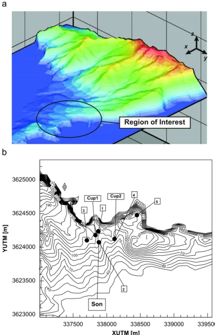
1000 m in width) in the east side of the Island, near the city of Canic-al. This area, 100 m above the sea level, which prolongs until the east end of the Island, is delimited by a cliff to the north, a relatively gentle slope towards the ocean to the south and a mountainous chain to the west (Fig. 1b). There was particularly interest in the suitability of five locations near the cliff (inTable 1) for installation of wind turbines, within a rectangle of 762411 m.
The most reliable long-term wind data in Madeira Island have been collected at the airport of
Santa Catarina(28 334 360 3 617 616N). The mean wind speed in the airport for a 10-year period
XUTM [m]
YUTM [m]
337500 338000 338500 339000 339500 3623000
3623500 3624000 3624500 3625000
Cup1 Cup2
Son
x
y z
Fig. 1.Three-dimensional view of the East region of the Madeira Island, showing the Sa˜o Lourenc-o Cape, and region of interest,
(1971–1980) was equal to 4:8 m s1European Wind Atlas(Troen and Petersen, 1989). However, the 8 km distance between the airport and the area of interest is too large for a confident use of measure–correlate–predict (MCP) methodologies; given the complexity of the local terrain and the nearby mountains in the SW–N directions, which have a pronounced influence on the air flow with large fluctuations of the wind direction (cf.Troen and Petersen, 1989, p. 402).
2.2. Cup and sonic anemometers
During the field campaigns in the area, three cup anemometers (Cup1, Cup2, and Cup3, inTable 2) were used. Cup1 and Cup2 were NRG systems (anemometer model 40 and data logger 9100 Plus), operating at a sampling frequency of 0.5 Hz, and with mean and standard deviation of velocity stored at every 10 min period. The mean wind direction was also known at Cup1 (40 m) and Cup2 (10 m). The sonic anemometer (Metek USA-1) was installed 47 m above ground level (agl) at location 2 (Table 1) thought to be representative of the wind conditions in the region. The signal from the sonic anemometer, operated at 20 Hz sampling frequency, was stored in a portable computer, which also controlled and monitored the data acquisition process. The anemometer was previously calibrated in a wind tunnel with an error of 0.1%, for a velocity range between 4 and 16 m s1(Ribeiro, 2005).
2.3. Linear model (WAsP)
The WAsP computer code is widely used by the wind energy community, and there is no need for a detailed description of this code developed by the RISØ National Laboratory in Denmark. The reader may refer to the published literature (cf.Mortensen et al., 2004). WAsP is based on linearised forms of the fluid flow equations and its most fundamental assumptions do not differ much from other approaches such as MS3DJH (Mason and Sykes, 1979), both built on the seminal work ofJackson and Hunt (1975). These models underpredict the wind speed reduction and cannot predict flow separation (Ayotte and Hughes, 2004; Castro et al., 2003) in the lee-side of the hills (not to mention mountains), and are clearly unsuitable for complex terrain. Because they require modest computer resources and complex terrain was often avoided for turbine siting, these models became the reference tool among the wind energy engineering community, which is often using them beyond their range of validity (Bowen and Mortensen, 2004). Obviously there is a high level of uncertainty and risk when using linearised models under these conditions. A comparative analysis will be performed here, to illustrate how different the results obtained by the linear model can be.
Table 1
Location of the five points of interest and RIX index
No. Easting Northing Z RIX
1 337 875 3 624 235 99 22
2 337 876 3 624 071 97 17
3 337 708 3 624100 107 19
4 338 113 3 624128 88 20
5 338 464 3 624 483 120 33
Table 2
Cup and sonic anemometer measurements
Start and end dates Anemometer Easting Northing zagl
98:08:03–99:01:05 Cup1 337 830 3 624 180 10, 40
98:08:01–98:11:12 Cup2 338 120 3 624 135 10
2.4. Nonlinear (CFD) model
The continuity (1), the momentum (2) and the turbulence model equations (3) and (4) were written in tensor notation for a generic coordinate system, defined by transforming a physical Cartesian coordinate systemxiinto a computational systemxi:
qðruibkiÞ
qxi ¼0, (1)
qðrJuiÞ
qt þ
q
qxjðrukuib
j
kÞ ¼
q
qxjðpb
j
iÞ þ
q
qxj½ðtkiþskiÞb
j
k, (2)
where
tki¼
m J
quk
qxmb
m
i þ
qui
qxmb
m k
and
ski¼
2 3rkdkiþ
mt J
quk
qxmb
m
i þ
qui
qxmb
m k
.
The eddy viscosity was given bymt¼rCmk2=, wherekand, the turbulence kinetic energy and its
dissipation rate, were determined by
qðrJkÞ
qt þ
q
qxjðrukkb
j
kÞ ¼
q
qxj 1
J mþ mt sk
qk
qxmb
m
kb
j k
þJðPkrÞ (3)
and
qðrJÞ
qt þ
q
qxjðrukb
j
kÞ ¼
q
qxj 1
J mþ mt s
q
qxmb
m
kbjk
þJ C1 k Pk
C2r2 k
, (4)
where
Pk¼ski
1
J
quk
qxmb
m
i , (5)
C1¼1:44; C2¼1:92; Cm¼0:033; sk¼1:0; s¼1:85.
In the above equations,uiandpare the ensemble Reynolds-averaged velocities and pressure,randm
are the air’s density and molecular viscosity,Jis the determinant of the Jacobian matrix andbjk¼
Jqxj=qxkare the co-factors of the coordinate transformation. The transport equations (3) and (4) and
constantsC1;C2andskwere set as inLaunder and Spalding (1972), whereas the constantsCmands followed the recommendations byBeljaars et al. (1987). Due to the low altitude, the size of the integration domain (Section 2.4.1) and the relatively high wind speeds that we were interested in, both the stratification and the Coriolis effects were ignored.
The transport equations (1)–(4) were discretised by finite volume techniques, using a second-order, three-time level implicit scheme for time discretisation and a central-differencing scheme for spatial discretisation of the diffusive terms. The advective terms were discretised by the hybrid scheme, and a third-order truncation scheme, in case of the momentum equations (2). At each time-step (1 s), the resulting set of coupled algebraic equations was solved using the SIMPLE algorithm to dimensionless residuals below 5104. The simulations were carried on until reaching a periodic or a steady state. A discussion of the numerical techniques can be found for instance inFerziger and Peric´ (2002). The methodology described above is embodied in the computer code named VENTOSs
(cf.,Lopes da Costa et al., 2006; Castro et al., 2003; Castro and Palma, 2002).
2.4.1. Numerical mesh, boundary and initial conditions
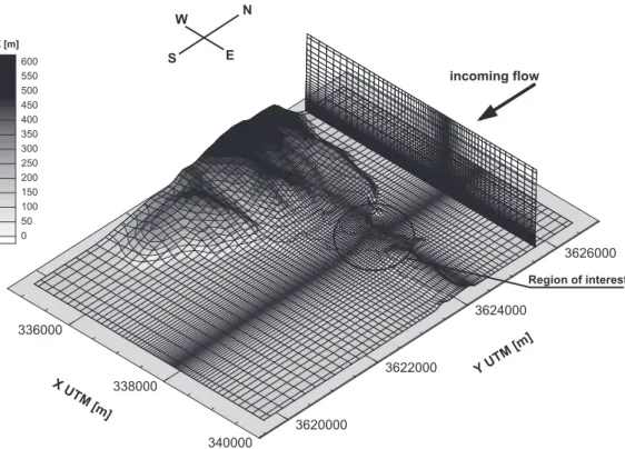
70005000 m,Fig. 2. The top boundary was set at 1500 m above sea level. A numerical mesh with 717151 grid nodes was used, centred at the region of interest and expanded along thex,yandz
directions, with factors of, respectively, 1.09, 1.13 and 1.09, with a minimum horizontal spacing equal to 20 m and the first vertical node at 1 m above the surface. Calculations were also made taking into account the terrain changes mentioned above (Section 1), determined by topographic survey of the terrain.
The bottom boundary was modelled by a rough surface, using wall laws (Launder and Sharma, 1974), assuming a region of constant tangential Reynolds stressst¼ru2 and a log-law tangential velocityut¼u=klnð1þz=z0Þ, wherek¼0:4 is the von Ka´rma´n constant,uis the friction velocity andzis the distance above the surface with characteristic roughnessz0, equal to 0.03 and 0.0002 m for land and sea surfaces. In the first control volume above the surface, wall laws were applied based on the relationshipsu2
¼kC
1=2
m andwall¼u3=½kðzþz0Þ.
The pressure at the boundaries was obtained by linear extrapolation from the inner nodes. The velocity was tangential at the top and lateral boundaries. The velocity outflow condition was obtained by linear extrapolation from the inner nodes, constrained by global mass conservation. For inlet boundary condition, a logarithmic boundary layer developed for a distance of about 2000 m over the ocean surface, with heightd¼1000 m and a free-stream velocity equal to 11:6 m s1. The turbulence kinetic energy and its dissipation rate at the inlet were determined by
k¼ ‘ 2
m C1=2
m u L 2
and ¼‘2m u L 3
,
where‘m¼minfkðzþz0Þ;Cmdg, andL¼kðzþz0ÞifzodorL¼d, ifzXd.
The computational domain size and both the grid size and distribution were established on the basis of the authors experience in the computer simulation of atmospheric flows (e.g.Castro, 1997;
X UTM [m]
336000
338000
340000
Y UTM [m]
3620000
3622000
3624000
3626000 600
550 500 450 400 350 300
250 200 150 100 50 0 Z [m]
incoming flow
Region of interest
N W
S E
Maurizi et al., 1998; Castro et al., 2003; Lopes da Costa et al., 2006; Silva Lopes et al., 2007) and within the capabilities of today’s personal computers, i.e. the hardware requirements of linear models. A highly accurate terrain discretisation over the whole extent of the domain, as shown inFig. 1, besides not being possible within the current computer limitations, was found unnecessary since the major features of the wind flow could be captured by the present arrangement. Computer simulations of atmospheric flows can be useful even when performed under conditions of low resolution, as recently pointed out byEidsvik (2008).
3. Discussion of results
3.1. Field measurements: cup anemometers
Based on different measuring periods, inTable 2, Cup2 at 10 m agl displayed a wind speed equal to 7:9 m s1, which was always higher than the wind speeds, 4.9 and 6:5 m s1, at Cup1 at 10 and 40 m agl, inTable 3, and well above the 4:8 m s1measured at the airport of Santa Catarina between 1971 and 1980 (Section 2.1). The wind was mostly from North, within 345 and 15, with a percentage above 70%. Turbulence intensity exceeded 20%, in the case of Cup1 at 10 m agl.
Simultaneous data at Cup1 and Cup2 were available only for a short period of 96 days and showed a consistently higher wind speed of 7:7 m s1 at Cup2, compared with 5:2 m s1 at Cup1 (Table 4). Such a large difference between the wind speeds at two stations only 300 m apart is most surprising.
Station inter-comparison is a powerful tool used in these circumstances, and its results are shown inTable 4using a format that departs from the usual one in the European Wind Atlas (Troen and Petersen, 1989). We show all combinations of predicted values at one point, in columns, based on measured field values at another point, in rows, including its own, in the main diagonal; for instance, using as input the wind conditions at Cup1 (10 m), wind speeds equal to 5.7, 5.3 and 5:0 m s1 are predicted, respectively, at Cup1 (40 m), Cup1 (10 m) and Cup2 (10 m), with relative errors with respect to the measured quantities of 9.6%, 1.9% and3:8%. The difficulty in predicting the values at one station based on the experimental data at a neighbouring station is obvious. Predictions of wind speed at mast Cup1, based on quantities measured at the mast, differed from the measured quantities in 9.6% and 4.3% if based on field quantities at a different height, and 2.9% or 1.9% if the both input and predicted quantities are referred to the same height. The latter, where the stations are predicting themselves, is often used as an indicator of abnormal behaviours, which can due to many different causes, such as data inconsistencies or wind flow behaviour.
Table 3
Wind speedðm s1Þand turbulence intensity (%)
Cup1 (10 m) Cup1 (40 m) Cup2 (10 m)
V 4.9 6.5 7.9
it 20.6 15.4 14.9
Table 4
Inter-comparison between meteorological stations (wind speed in m s1and relative error, in %, within parenthesis)
Station Measured Predicted
Cup1 (40 m) Cup1 (10 m) Cup2 (10 m)
Cup1 (40 m) 6.9 7.1 (2.9) 6.6 (4.3) 6.3 (8.7)
Cup1 (10 m) 5.2 5.7 (9.6) 5.3 (1.9) 5.0 (3.8)
The results in Table 4 show that none of the locations provides a good representation of the wind field in the area and the use of the methodology embodied in the WAsP computer is questionable.
Analysis of the field data revealed sudden changes of the wind direction. We counted the number of 30sectors between consecutive 10 min periods, i.e. the wind direction did not change (0, zero), or change 1;2;3;4 and 5 sectors of 30, in Table 5. Changes of directions that spanned over 120 represented 2.3% of the whole data set Cup1 (40 m) and were more frequent than 30(2.1%) changes; at Cup1 at 40 m agl, the percentage of 120 changes is higher than all changes of direction at Cup2 (10 m). When the analysis was restricted to the period of simultaneous measurements at both masts, the distribution did not change much, and we concluded that this was a real feature of the wind in these two locations.
Such a drastic change, i.e. a reverse of direction, cannot be due to changes of weather conditions (mesoscale) nor turbulence, but a rather local phenomenon most likely induced by local features of the terrain. This also indicated the likely presence of a separated flow region, case under which the appropriateness of this area for installation of a wind park should be ruled out. Furthermore, the conventional techniques and procedures used in wind resource evaluation are not meant for this type of wind flow and may underestimate the turbulence intensity.
3.2. Field measurements: sonic anemometer
The sonic measurements were performed between the 12:35 of 10th and 11:35 of 11th October 2001, i.e. a total of 23 h with small interruptions to check the data acquisition process. The upper part
Table 5 Number of 30
sectors between consecutive sets of 10 min measurements (histogram)
No. of sectors
Cup1 (40 m) Cup2 (10 m) Cup1 (40 m) Cup2 (10 m)
Time [98:08:01
00:00–98:11:12 16:10]
[98:08:03
10:20–99:01:05 03:00]
[98:08:03 10:20–98:11:12 16:10]
0 16 467 (89.6) 13 247 (96.0) 11 598 (88.3) 12 916 (96.1)
1 392 (2.1) 139 (1.0) 278 (2.1) 139 (1.0)
2 184 (1.0) 32 (0.2) 140 (1.1) 32 (0.2)
3 338 (1.8) 27 (0.2) 286 (2.2) 27 (0.2)
4 420 (2.3) 15 (0.1) 391 (3.0) 15 (0.1)
5 77 ( 0.4) 11 (0.1) 75 (0.6) 11 (0.1)
Percentual values within parenthesis.
Table 6
First to fourth moments of the totalðvÞ, horizontalðvhÞand vertical velocityðvzÞfrom 2001 October 10th, 12:35 to 11th, 11:35, with data sampling at 20 Hz
x [Min, Max] s Skewness Kurtosis
v 10.33 [0.03, 29.87] 3.94 0.34 2.22
vh 9.89 [0.00, 28.54] 4.29 0.37 2.10
vz 0.49 [18.75, 22.29] 2.38 0.28 4.65
vw 10.33 [5.61, 14.20] 1.95 0.29 2.46
itw 0.34 [0.10, 0.54] 0.12 0.45 2.24
Gw 2.12 [1.27, 3.78] 0.54 0.87 3.54
ofTable 6includes the first four statistical moments over the whole 23 h, during which the mean wind velocity was from the north quadrant and equal to 10:33 m s1, with horizontal and vertical components of 9.89 and 0:49 m s1. The vertical velocity, v
z, displays a much different behaviour
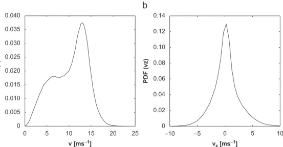
compared withvandvh, as evidenced by a kurtosis equal to 4.65 (higher than the Gaussian value of 3) and unbalanced in favour of values above the average (a positive skewness). However, the most striking result is the velocity range on the vertical plane, with values between 18:75 and 22:29 m s1. The lower kurtosis of the horizontal velocity (2.10) is explained by the nearly bimodal PDF (Fig. 3a); this is an indication of the presence of events with distinct time scales, to be found by frequency analysis.
The lower part ofTable 6includes the three major parameters, the mean velocityv, the turbulence intensityit¼sðvÞ=vand the gust factorG, averaged over a 10-min period, as recommended in wind energy resource studies (IEA, 1999). The mean turbulence intensity itw was 34% with a standard
deviation of 12%, andGwas 2.12 with a standard deviation of 0.54. Both the turbulence intensity and the gust factor are too high and exceed the design values of standard wind turbines (IEC, 1999, 2003; Burton et al., 2001).
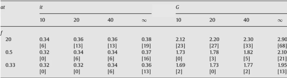
For a site with a turbulence level so high, the sampling frequency and the integration time for statistical analysis are critical, namely when we are interested also in higher-order statistical moments. The sonic anemometer time series was re-sampled with a low-pass anti-aliasing FIR filter at 0.33 and 0.50 Hz to mimic the measurements of cup anemometers with different time constants, 3 and 2 m, where the latter is close to the parameters of operation of the NRG (model 40) cup anemometer. The integration, averaging timeatfor statistical analysis was 10, 20, 40 min and the whole 23 h period (denoted by 1). Table 7 shows, as expected, that the range of values of any variable is reduced when decreasing the sampling rate. Because it is a function of the maximum, the consequences are greater on the gust factor, which is equal to 2.90, 2.10 and 1.95 for sampling frequencies, respectively, of 20, 0.5 and 0.33. A maximum difference of 68% occurs in the determination of the gust factor, whereas the turbulence intensity shows values between 0% and 19%, depending on the sampling frequency and averaging time.
The simple statistical analysis inTable 6is not appropriate for inferring on the existence (or not) of a wide region of separated flow, and spectral analysis was also used, inFig. 4. For comparison with the computational results (in Section 3.4), a transect of the time series that presented lower unsteadiness was selected and divided into sets of 10, 20 and 40 min, i.e., respectively, 32, 16 and 8
0 5 10 15 20 25
0 0.005 0.010 0.015 0.020 0.025 0.030 0.035 0.040
v [ms−1]
PDF (v)
−10 −5 0 5 10
0 0.02 0.04 0.06 0.08 0.10 0.12 0.14
vz [ms−1]
PDF (vz)
blocks of identical duration, each post-processed referring to a constant wind speed in streamline coordinates. The mean value of each data set was extracted after rotation to avoid interferences from low-frequency events in the spectra (cf.Kaimal and Finnigan, 1994). Common to all time intervals are
0 200 400 600 800 1000 1200 1400 1600 1800 2000
S(u)/
σ
(u)
2
0 500 1000 1500 2000 2500 3000 3500 4000
10−1 100 101 102 10−1 100 101 102
T [min] T [min]
10−1 100 101 102 10−1 100 101 102
T [min] T [min]
S(u)/
σ
(u)
2
0 500 1000 1500 2000 2500
S(u)/
σ
(u)
2
0 500 1000 1500 2000 2500 3000 3500 4000 4500 5000
S(u)/
σ
(u)
2
Fig. 4.Normalised spectra for a 320-min data record reconstructed with detrended data for (a) 3210-min, (b) 1620-min, (c) 840-min time intervals, and (d) whole series.
Table 7
Turbulence intensityitand gust factorGas a function of sampling ratesfin Hz and averaging timeatin minute
at it G
10 20 40 1 10 20 40 1
f
20 0.34 0.36 0.36 0.38 2.12 2.20 2.30 2.90
[6] [13] [13] [19] [23] [27] [33] [68]
0.5 0.32 0.34 0.34 0.37 1.73 1.78 1.82 2.10
[0] [6] [6] [16] [0] [3] [5] [21]
0.33 0.32 0.32 0.34 0.36 1.69 1.73 1.77 1.95
[0] [0] [6] [13] [2] [0] [2] [13]
a set of high peaks between 5 and 8 min, which can be a single period (8 min) in the case ofFig. 4b. The 10-min interval was selected based on the established practise in wind resource evaluation and meteorological data analysis.
3.3. Computational results: linear model (WAsP)
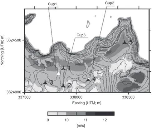
Fig. 5 shows the horizontal velocity, at 40 m agl, as predicted by the linear model WAsP (version 6), under neutral stability conditions. As expected, the results were strongly correlated with the terrain elevation and the high velocity regions (around 12 m s1) appeared around the edges of the cliff, near locations 1 and 5. The wind speed at locations 2, 3 and 4 was about 10 m s1.
The RIX (ruggedness index) is the percentage fraction of the terrain along the prevailing wind direction above a critical slope of 0.3; it was created in an attempt to quantify the terrain complexity and therefore enable a more accurate definition of the conditions under which the WAsP code could be used (Bowen and Mortensen, 2004). The RIX, inTable 1, varied between 17 and 33, for locations 5 and 2, and was above the limits of applicability of the linear models. Under these conditions, the linear models if used, should be used very cautiously.
3.4. Computational results: nonlinear model
Simulations were performed for southerlyð180
Þ, northerlyð0
Þand north-easterlyð22:5Þwinds. There was a total of four different cases, counting on an additional northerly wind simulation, to take into account recent terrain changes.
Cup1 Cup2
Cup3 3624500
3624000
337500 338000 338500
Northing [UTm; m]
Easting [UTM; m]
9 10 11 12
[m/s]
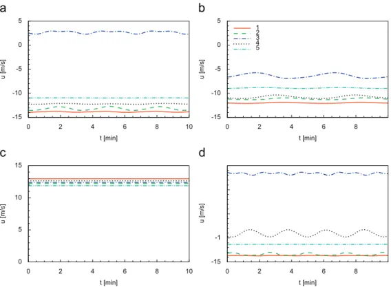
3.4.1. Time series
The temporal evolution of the longitudinal velocity is shown inFig. 6for all five locations and the four cases being simulated. In case of southerly winds (Fig. 6c), there was a constant wind velocity of a similar magnitude for all five locations. This was a simple consequence of the topography, with no cliff on the south side and no major obstacle to southerly winds (seeFig. 1).
Concerning the northerly and north-easterly winds (Figs. 6a, b and d), differences of 18 m s1between wind velocities could be reached (14 and 4 m s1, in locations 1 and 3,Fig. 6d). In case of northerly winds (Figs. 6a and d), the direction of the velocity in location 3 was opposite to all the remaining locations. The time dependency of the wind velocity was restricted to locations 2, 3 and 4, which, though only about 200 m away from 1 and 5, are already in the descending part of the terrain (Fig. 1b).
The terrain changes performed after the cup anemometer measurements enhanced the time-dependent behaviour (compareFigs. 6d and a); the velocity amplitude (the largest amplitude of all) in location 4 increased and the 1-min period of the oscillation in location 3 was 2lower than in locations 4 or 1. This depended much on the direction of the prevailing winds and in case of north-easterly winds (Fig. 6b), for instance, there was no reversed flow in location 3 and the period changed to 7 min. The periods of oscillation are well in agreement with the spectral analysis of the sonic anemometer, in Section 3.2.
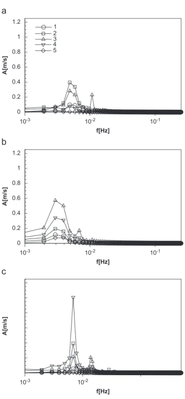
The frequency analysis inFig. 7enables a more accurate determination of the frequencies in the time series, whose peak occurs at 5, 3 and 7103Hz (periods equal to 3.3, 5.6 and 4.2 min), respectively for northerly, north-easterly, and northerly winds after terrain changes (Figs. 7a, b and d), which magnified the amplitude of the oscillation by a factor of two (cf.,Fig. 7d, against a and b). Not all locations are equally prone to low frequency unsteadiness of the wind flow, which depends much on the wind flow direction; in any case and based on the four conditions being tested, one may conclude that locations 1 and 5 (the locations nearest to the cliff) are the less likely to suffer from this
t [min]
u [m/s]
0 2 4 6 8 10
-15 -10 -5 0 5
t [min]
u [m/s]
0 2 4 6 8
-15 -10 -5 0 5
1 2 3 4 5
t [min]
u [m/s]
0 2 4 6 8 10
0 5 10 15
t [min]
u [m/s]
0 2 4 6 8
-15 -1
A[m/s]
10-3 10-2 10-1
0 0.2 0.4 0.6 0.8 1 1.2
1 2 3 4 5
f[Hz]
A[m/s]
10-3 10-2 10-1
0 0.2 0.4 0.6 0.8 1 1.2
f[Hz]
f[Hz]
A[m/s]
10-3 10-2
problem compared to locations 3, 2 and 1, located further downstream. The computer simulation with a constant wind speed could not be accurately replicate the actual wind conditions, with unstationary time series. Under these conditions, there is a fair agreement between the peak periods predicted by the computer simulations, 3.3, 4.2 and 5.6, and those found by sonic measurements, between 5 and 8 min, in Section 3.2.
The real atmospheric flow showed a nonstationary behaviour, whereas the simulations presented simple periodic results, due to, among other factors, the nonexistence of mesoscale forcing of the model. The frequencies predicted by the model can be related only with the natural (low) frequency of the recirculation regions.
Given the time dependency of the wind flow in some areas of the integration domain, the following numerical results were time-averaged for at least 20 min, to include 3–20 complete periods of the low frequency unsteadiness inFig. 6.
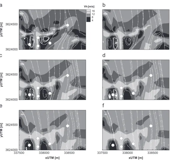
3.4.2. Flow pattern
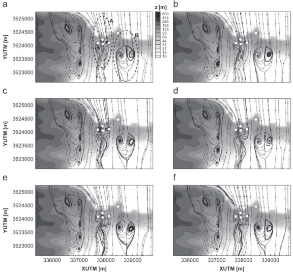
A global view of the flow (northerly wind) for four different heights is presented inFig. 8. We start by noting the complexity of the flow pattern as displayed by the stream traces and the large
xUTM [m]
yUTM [m]
337500 338000 338500 3624000
3624500
xUTM [m] 337500 338000 338500
yUTM [m]
3624000 3624500
yUTM [m]
3624000 3624500
16 12 8 4 Vh [m/s]
differences in wind velocity between the five locations, despite their proximity of only a few hundred metres. At 20 m agl (Fig. 8b) there are three vortices: two counter-rotating ones around location 3, and a third vortex close to location 4. These three vortices decelerate the incoming upstream (northerly) wind—a blockage effect—creating an extended region of higher velocity aligned with
locations 1 and 2. The vortices around location 3 are the strongest, showing even at 60 m agl (Fig. 8f); this explains why in case of northerly winds, the wind direction in location 3 was from south to north (Figs. 6a and d), contrary to the wind direction in any of the remaining four locations. The presence of those three vortices also explains why the locations 2, 3 and 4 exhibited the larger amplitudes of the time-dependent oscillations. These locations are further away from the coastline compared with locations 1 and 5, in a descending part of the terrain, partly covered by the terrain upstream and therefore with favourable conditions to flow separation (Fig. 1).
In an attempt to illustrate the dynamics of the flow in this region, we show a sequence of frames Dt¼60 s apart, inFig. 9. Here, because we are showing a larger region compared with that inFig. 8, the effect of the mountains located west of the site (seeFig. 1also) is most obvious, via the curvature of the streaklines in the lower left corner. All regions, except D, display a time-dependent behaviour. This is most obvious first around region A, and less intense around regions B and C. The flow
XUTM [m]
336000 337000 338000 339000
YUTM [m]
3623000 3623500 3624000 3624500 3625000
XUTM [m]
YUTM [m]
336000 337000 338000 339000 3623000
3623500 3624000 3624500 3625000
YUTM [m]
3623000 3623500 3624000 3624500 3625000
600 414 285 196 135 93 64 44 31 21 15 10 z [m]
B A
structure in A and B is due to the terrain slope and the location in the lee-side of either the cliff (region A) or the elevated terrain (region B).
The vortex chain in region C is the result of the interaction between part of the flow around and part of the flow coming down (mountain flows) the mountain chain (inFig. 1). The double-vortex structure in B evidences a cyclic pattern (at a low frequency), typical of separated flow region. There is a time when the streaklines increase their density and all seem to converge towards the centre of the vortex system, followed by a sudden burst that propagates downstream leading to the wave-like behaviour. This can also be observed for each of the four vortices contained in region C; however, this behaviour is much stronger in region A, particularly at location numbered 3, in the centre of the vortex.
The onset of separation behind hills is of great practical importance in both wind energy and atmospheric dispersion problems, and a few guidelines are available based on the critical slopeðycritÞ for flow separation.Wood (1995)for instance gives an overview on previous work and proposes a simple expression for determining ycrit based on the terrain roughness and hill width, which if applied to the present case, assuming a hill width and a characteristic roughness equal to 1000 and 0.03 m, would yieldycrit¼18:7.
In summary, this is a flow pattern rich in critical points, some of which are unstable and the reason for the flow time dependence. The global view and details provided by the three-dimensional flow calculations are unsurpassed, and could never be obtained by any point measurement technique being used. Because of its mathematical model, WAsP also could not capture the flow nor the vortices structures associated with flow separation, and the wind flow in the lee-side of the cliff is much different from that predicted by the CFD nonlinear model.
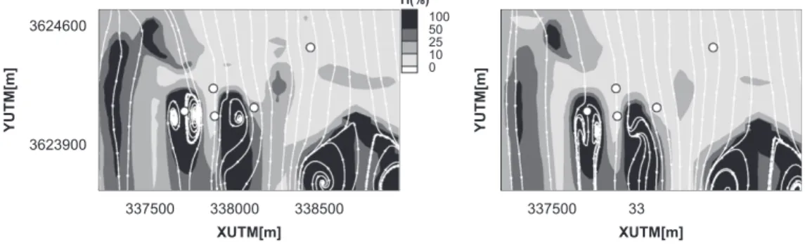
3.4.3. Turbulence intensity
The effect of turbulence on the operation of the wind turbines is difficult to predict, and quantify. High turbulence can affect the electricity production, increase the probability of malfunctions and reduce the equipment life-time. A turbulence intensity equal to 16% or 18%, depending on the turbine class, has been established as the design condition for wind turbines (cf., IEC, 1999). For a discussion on the current practise and standards you may refer to Burton et al. (2001, Section 2.6.3, p. 21).
Under normal conditions, turbulence is reduced as we approach the top of the hill and low turbulence goes together with high wind velocity. Small scale topography, mesoscale phenomenon, steep slopes and flow separation may all change the situation described above. The turbulence intensity (Fig. 10) is lower along the cliff and locations 1 and 5 do not suffer from problems associated with high turbulence, contrary to locations 3 and 4. The turbulence intensity at location 3 shows an abnormal behaviour, since it decreases with the distance to the ground. The turbulence intensity here is set mainly by the flow separation and the maximum occurs in the shear layer at around 100 m above the ground (see vertical profiles, inFig. 11). The turbulence intensity depends much on the separated flow region downstream of the cliff, and can reach values in excess of 100%.
XUTM[m]
YUTM[m]
337500 338000 338500 3623900
3624600 10050
25 10 0 Ti(%)
XUTM[m]
YUTM[m]
337500 33
3.4.4. Vertical profiles and shear factor
The transversal and vertical velocities (vandw) at location 3 (Fig. 11) are relatively low over the whole height, however, the vertical profiles of both the longitudinal velocity and the turbulence kinetic energy are unacceptable from the point of view of wind energy applications. In case of northerly wind, because location 3 was in the middle of a recirculation zone, theuvelocity reversed direction, changing from a nearly constant value of3 m s1in the first 40 m to 12 m s1for distances higher than 100 m agl. This high vertical gradient ofuwas accompanied by an increasing turbulence kinetic energy with a peak value equal to 11:2 m2s2atz¼60 m (Fig. 11a), i.e. 17compared with those in any of the remaining four locations and well beyond the design conditions of wind turbines. Location 5 did not show any periodic behaviour nor was located near a recirculation region (Sections 3.4.1 and 3.4.2) and above all the vertical profiles of either the longitudinal velocity or the turbulence kinetic energy (inFig. 12) did not display any of the unwanted features seen at location 3 (Fig. 11). However, at location 5 the vertical velocity of 2 m s1 was about 20% of the horizontal velocity, in case of northerly winds. Locations 5 and 1, though not evidencing time-dependent (periodic) behaviour, showed a high vertical velocity, which could reach 40% of the horizontal component in case of location 1, for north-easterly winds. These locations are too close to the cliff
u,v,w[m/s] k[m2/s2]
z[m]
-5 0 5 10 15 20
0 2 4 6 8 10 12 14
50 100 150 200
u v w k
u,v,w[m/s] k[m2/s2]
z[m]
-5 0 5 10 15
0
Fig. 11.Longitudinal, transversal and vertical (u,vandw) velocity components and turbulence kinetic energy. Ensemble-averaged values for location 3: (a) north; (b) north, after terrain changes.
u,v,w[m/s] k[m2/s2]
z[m]
0 10 20
0 2 4 6 8 10 12 14
101 102
101 102
u,v,w[m/s] k[m2/s2]
z[m]
0 10
0 2 4 6 8 10 12 1
and angles of about 20between the wind velocity and the horizontal plane are not acceptable for horizontal axis wind turbines. Acceptable behaviour was found only for southerly winds, when the wind flow was identical for all five locations, also well represented by the values in Fig. 12b for location 5. However, southerly winds are not so frequent in Madeira Island (Section 3.1).
The shear factor, defined asa¼logðu2=u1Þ=logðz2=z1Þ, is the key parameter used to extrapolate measurements at cup height to hub height and a1
7power law (i.e.a¼0:14) is usually assumed. This approach, however, was valid only above the sea surface. Negative shear factors occurred around location 3 for distances to the ground above 40 m, showing a decreasing horizontal velocity for larger distances to the ground.
4. Conclusions
The wind flow over a coastal region—a cliff over the sea—was studied by a wide variety of
techniques including field measurements with cup and sonic anemometer, and computer simulations using linear and nonlinear (CFD) mathematical models of the fluid flow equations.
Conventional measurements for wind resource assessment showed sudden variations of the wind direction and were a first indication of the presence of a complex wind pattern that cup anemometer point measurements could not fully uncover. Measurements with sonic anemometer revealed an energy spectrum with discrete peaks related with periodic events of a duration inferior to the 10 min averaging of conventional cup anemometer measurements. The results of the nonlinear (CFD) flow model compared favourably with field measurements and showed that three of the five locations under study for wind turbine location would be in the vicinity of reversed flow regions, characterised also by large turbulence intensity. These locations displayed a pulsating flow, with periods between 1 and 8 min, depending on the location and the wind prevailing direction. One of the locations, 200 m downstream of the cliff, was even in the centre of a vortex system and displayed the strongest oscillations. For northerly winds of about 15 m s1, within the first 40 m above the ground, the wind direction was reversed, from south to north. Under these conditions, conventional analyses as used in resource assessment was insufficient. Turbulence intensity and gust factors were poor estimators and depended strongly on sampling rate and time averaging period. In spite of large differences between the mean wind velocity at each of the five locations, the field measurements, at one single location, after appropriate analysis, contributed to our confidence in the computational results and an increased knowledge of the wind flow-field in the whole area of interest.The results presented here favour the usage of three-dimensional nonlinear (CFD) models as a complement to simpler models developed for wind flows over simple orography. The CFD calculations though not entering in the decision process that led to the selection of the place for field measurements, as they should, influenced the analysis of the field data, by revealing aspects left unnoticed by more traditional approaches and that were the first choice when studying the appropriateness of the area for installation of a wind farm.
Acknowledgements
References
Ayotte, K.W., Hughes, D.E., 2004. Observations of boundary-layer wind-tunnel flow over isolated ridges of varying steepness and roughness. Boundary-Layer Meteorol. 112, 525–556.
Beljaars, A.C.M., Walmsley, J.L., Taylor, P.A., 1987. A mixed spectral finite-difference model for neutrally stratified boundary-layer flow over roughness changes and topography. Boundary-Layer Meteorol. 38, 273–303.
Bowen, A.J., Mortensen, N.G., 2004. WAsP prediction errors due to site orography. Technical Report Risø-R-995(EN), Risø National Laboratory, Roskilde, Denmark, December.
Burton, T., Sharpe, D., Jenkins, N., Bossanyi, E., 2001. Wind Energy Handbook. Wiley, UK.
Castro, F.A., 1997. Numerical methods for the simulation of atmospheric flows over complex terrain. Ph.D. Thesis, Faculty of Engineering of the University of Porto (in Portuguese).
Castro, F.A., Palma, J.M.L.M., 2002. VENTOSs
: a computer code for simulation of atmospheric flow over complex terrain. Technical Report, Available from the authors, 21pp.
Castro, F.A., Palma, J.M.L.M., Silva Lopes, A., 2003. Simulation of the Askervein flow. Part 1: Reynolds averaged Navier–Stokes equations (k–turbulence model). Boundary-Layer Meteorol. 107, 501–530.
Eidsvik, K.J., 2008. Prediction errors associated with sparse grid estimates of flows over hills. Boundary-Layer Meteorol. 127 (1), 153–172.
Ferziger, J.H., Peric´, M., 2002. Computational Methods for Fluid Dynamics, third ed. Springer, Berlin.
IEC, 1999. Wind turbine generator systems—part 1: safety requirements. Technical Report, IEC-International Electrotechnical
Commission, Geneva, Switzerland, International Standard IEC 61400-1.
IEC, 2003. Wind turbine generator systems—part 1: design requirements. Technical Report, IEC-International Electrotechnical
Commission, Geneva, Switzerland, International Standard IEC 61400-1 Ed.3.
Jackson, P.S., Hunt, J.C.R., 1975. Turbulent wind over a low hill. Q. J. R. Meteorol. Soc. 101, 929–955.
Kaimal, J.C., Finnigan, J.J., 1994. Atmospheric Boundary Layer Flows. Their Structure and Measurement. Oxford University Press, Oxford.
Landberg, L., Myllerup, L., Rathmann, O., Petersen, E.L., Jørgensen, B.H., Badger, J., Mortensen, N.G., 2003. Wind resource estimation—an overview. Wind Energy 6, 261–271.
Launder, B.E., Sharma, B.I., 1974. Application of the energy-dissipation model of turbulence to the calculation of flow near a spinning disc. Lett. Heat Mass Transfer 1, 131–138.
Launder, B.E., Spalding, D.B., 1972. Mathematical Models of Turbulence. Academic Press, London.
Lopes da Costa, J.C., Castro, F.A., Palma, J.M.L.M., Stuart, P., 2006. Computer simulation of atmospheric flows over real forests for wind energy resource evaluation. J. Wind Eng. Ind. Aerodyn. 94 (8), 603–620.
Mason, P.J., Sykes, R.I., 1979. Three-dimensional numerical integrations of the Navier–Stokes for flow over surface-mounted obstacles. J. Fluid Mech. 91, 433–450.
Maurizi, A., Palma, J.M.L.M., Castro, F.A., 1998. Numerical simulation of the atmospheric flow in a mountainous region of the North of Portugal. J. Wind Eng. Ind. Aerodyn. 74–76, 219–228.
Mortensen, N.G., Landberg, L., Troen, I., Petersen, E.L., Rathmann, O., Nielsen, M., 2004. WAsP utility programs. Technical Report Risø-R-995(EN), Risø National Laboratory, Roskilde, Denmark, September. URL:hwww.wasp.dki.
NREL, 1997. Wind resource assessment handbook: fundamentals for conducting a successful monitoring program. Technical Report, NREL—National Renewable Energy Laboratory, Golden, CO, NREL Subcontract N. TAT-5-15283-01.
Pedersen, B.M., Pedersen, T.F., Klung, H., van der Borg, N., Kelley, N,. Dahlberg, J.A˚., 1999. Wind speed measurement and use of cup anemometry. In: Hunter, R.S. (Ed.), Expert Group Study on Recommended Particles for Wind Turbine Testing and Evaluation, vol. 11, first ed. International Energy Agency.
Piomelli, U., Balaras, E., 2002. Wall-layer models for large-eddy simulations. Annu. Rev. Fluid Mech. 34, 349–374. Pope, S.B., 2000. Turbulent Flows. Cambridge University Press, Cambridge.
Raithby, G.D., Stubley, G.D., Taylor, P.A., 1987. The Askervein hill project: a finite control volume prediction on three-dimensional flows over the hill. Boundary-Layer Meteorol. 39, 107–132.
Ribeiro, L.M.F., 2005. Sonic anemometer and atmospheric flows over complex terrain. Ph.D. Thesis, University of Porto, Portugal.
Silva Lopes, A., Palma, J.M.L.M., Castro, F.A., 2007. Simulation of the Askervein flow. Part 2: large-eddy simulations. Boundary-Layer Meteorol. 125, 85–108.
Spalart, P.R., Jou, W.H., Strelets, M., Allmaras, S.R., 1997. Comments on the feasibility of LES for wings and on a hybrid RaNS/LES approach. In: Liu, C., Liu, Z. (Eds.), Advances in DNS/LES. Greyden, Colombus, OH, USA, pp. 137–148.
Troen, I., Petersen, E.L., 1989. European Wind Atlas. Risø National Laboratory, Denmark.
Wood, N., 1995. The onset of separation in neutral, turbulent flow over hills. Boundary-Layer Meteorol. 76, 137–164. Wood, N., 2000. Wind flow over complex terrain: a historical perspective and the prospect for large-eddy modelling.