Antonio Soares Martins Neto Economic Commission for Latin America and the Caribbean
Resumo
Durante o boom das commodities, o Brasil au-mentou sua especialização em matérias-primas, ao mesmo tempo em que reduziu a desigualdade de renda (através de diversas políticas distributi-vas). Além disso, o crescimento da produtividade foi insufi ciente durante o mesmo período. Esta trajetória é insustentável não somente no médio prazo, mas também pode ter afetado o cresci-mento brasileiro consistente com o equilíbrio ex-terno. O presente artigo discute, através de um modelo macrodinâmico baseado em Ribeiro et al. (2016), o impacto dos programas de distribuição de renda no crescimento brasileiro. Sugere-se que os programas distributivos podem prejudicar o crescimento de longo prazo devido ao aumento da elasticidade-renda das importações e ao aumento da brecha tecnológica. Por fi m, argumenta-se que o equilíbrio entre investimento público e progra-mas distributivos permitiria um ciclo virtuoso de crescimento e distribuição de renda.
Palavras-chave
crescimento sob restrição externa; distribuição de renda; investimento público.
Códigos JELE25; E62; O33; O40. Abstract
Within the commodities price boom, Brazil experienced rising dependency on primary exports, along with falling inequality (as a result, among others, of extensive distributive programs). However, productivity growth was meager during the period. Not only this path is unsustainable in the medium run, but may also have harmed the long-run growth consistent with BOP equilibrium. This paper discusses, in a BOP-dominated macrodynamic model based on Ribeiro et al. (2016), the impact of Brazilian distributive policies in the BOP-constrained rate of growth. It is suggested that distributive programs can harm long-term growth due to rising income elasticity of imports and higher technological gap. Lastly, it is argued that the right balance of public investment and distributive programs would allow a virtuous cycle of growth and income distribution to emerge.
Keywords
BoP-constrained growth model; income distribution; public investment.
JEL CodesE25; E62; O33; O40.
Income distribution and external constraint:
Brazil in the commodities boom
1
Introduction
Brazil embarked in an extensive distributive program in the 2000s, focus-ing on minimum wage and cash transfer programs. Supported by favorable external conditions (commodities price boom), the country experienced sus-tainable growth along with falling inequality. However, in the meantime, Brazil became more dependent on export of commodities to Asian markets. Eventually, when the commodity lottery reversed, a stagnant productivity growth and rising current account defi cits exposed Brazilian weaknesses.
This path of falling inequality, low productivity and rising dependence on primary goods is unsustainable (see Cimoli et al., 2015). If productivity does not grow steadily, the potential to increase social expenditure to fi ght poverty and encourage social inclusion will fi nd a ceiling. Slow productiv-ity growth along with rising wages compromises competitiveness, which in turn heightens the external constraint and compromises growth.
The impact of income distribution on non-price competitiveness in a BOP-constrained framework is a recent development in the post-Keynes-ian literature.1 Porcile et al. (2007) discuss how a rise in real wages may boost non-price competitiveness. The tale is quite simple: up to a cer-tain critical point, higher real wages enhance the ability of workers to learn, imitate and improve foreign technology, with positive effects on non-price competitiveness. Ribeiro et al. (2016) discuss several channels through which an exchange rate policy may affect non-price competitive-ness. Among them, the paper discusses how changes in the real exchange rate affect income distribution and how the latter infl uences consumption patterns and fi rms’ decisions.
However, some limitations appear in these works. First, in Porcile et al. (2007), there is no discussion of the impact of income distribution on consumption patterns and, then, on the income elasticity of imports. Sec-ond, in Ribeiro et al. (2016), even though the authors provide an extensive discussion on the effects in both income elasticities (and affi rm that “the net impact of changes in the wage share on each income elasticity can go either way…” (Ribeiro et al., 2016, p.12)), the ultimate assumption of a positive impact of income distribution on the trade elasticities ratio may not hold for the Brazilian economy (Souto, 2015).
Therefore, this paper aims to contribute to the literature on income dis-tribution, discussing its interactions with non-price competitiveness and growth. This paper discusses, in a BOP-dominated macrodynamic model based on Ribeiro et al. (2016), the impact of Brazilian distributive policies on the BOP-constrained rate of growth. Moreover, this paper includes a government sector as in Cimoli et al. (2015), which tax profi ts and spends in distributive programs and productive investment. As a result, the opti-mal balance between the two types of expenditures is discussed. Under some circumstances, policies that target income distribution will negative-ly affect long-term growth.
Therefore, the fi rst contribution of this paper is to present the condi-tions in which a rise in social expenditures can harm economic growth. We take the Brazilian economy as a background for our theoretical model and discuss how, in an economy with weak productive structure, a rise in distributive programs can affect the trade income elasticities and then the long-term growth consistent with the BOP equilibrium. On one hand, rising wages (when not compensated by a rise in productivity) curb in-novation, as they reduce fi rms’ profi ts.2 As a result, specialization in pri-mary goods (which normally have lower income elasticity of demand) is intensifi ed. On the other hand, if the rise in the demand for luxury goods by workers surpasses the fall in demand for luxury goods by capitalists, cash transfers and rising minimum wages lead to higher import elasticities. A second contribution of the paper is to discuss the importance of the complementarity between public investment and social expenditure. While the fi rst is important to reduce the technological gap and guarantee that the domestic supply meets the demand, the latter permits the distri-bution of the fruits of the rapid development. All in all, the right balance of public investment and distributive programs would allow a virtuous cycle of growth and income distribution to emerge.
The paper is organized in four sections, besides this introduction. Sec-tion 2 presents stylized facts of the Brazilian economy during the com-modity boom. Section 3 describes a BOP-constrained model in which in-come elasticities interact with inin-come distribution and labor cost. Section 4 discusses distributive policies and, also, the combination of distributive policies and public investment. A fi nal section concludes.
2
Stylized facts
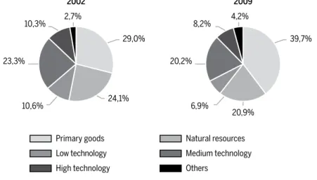
In a neo-Kaleckian perspective (Dutt, 1984; Bhaduri; Marglin, 1990), given different saving propensities, income distribution and economic growth walk side by side. This was the case of Brazil, where income distribu-tion, consumption and economic growth moved along (see, for instance, Serrano; Suma, 2012; Carvalho; Rugitisky, 2015). However, despite posi-tive short-run fl uctuations, during the commodity prices boom Brazil experienced rising specialization in primary goods, mostly in exports of commodities to Asian markets (see Figure 1). Most explanations of this process emphasize the role of an overvalued exchange rate (e.g., Oreiro
et al., 2012). From 2003 onward, Brazilian real exchange rate was kept
constantly overvalued (see Figure 2), which may have curbed manufac-turers’ profi tability and may have facilitated imports of consumption and luxury goods. However, along with an overvalued exchange rate, Brazil embarked in an extensive distributive program concentrated in rising min-imum wage and cash transfer programs (Serrano; Suma, 2012; Carvalho; Rugitsky, 2015).
Figure 1 Pattern of specialization – Brazilian exports grouped by technology 2002 and 2009
Source: Authors calculation based on UN Comtrade and Timmer et al. (2015).
Note: Values for 2009 are in 2002 constant prices. We defl ate each group by the average of the cor-responding industries using data from Timmer et al. (2015).
29,0%
24,1% 10,6%
23,3%
10,3% 2,7%
2002
Primary goods Natural resources Low technology Medium technology High technology Others
39,7%
20,9% 6,9%
20,2%
8,2% 4,2%
Figure 2 Real exchange rate, Brazil: 2000-2010
Source: Authors’ calculation based on Penn World Tables.
Note: As in Rodrik (2008), we build an undervaluation index. If the real exchange rate is negative (as it is from 2005-2010), it means that the real exchange rate is overvalued.
Certainly, income inequality is a topic of great relevance for Brazil - one of the most unequal countries in the world (ECLAC, 2016). In fact, during the commodity boom that started in 2004, Brazil experienced, for the fi rst time since the Second World War, a period of rapid economic growth ac-companied by a fall in inequality – the Gini index in Brazil fell from 58.7 in 2002 to 52.6 in 2012, while GDP growth rate averaged almost 4%.3 The most successful Brazilian program was Bolsa Família, which became an exemplary policy around the region and helped millions surpass the poverty line.
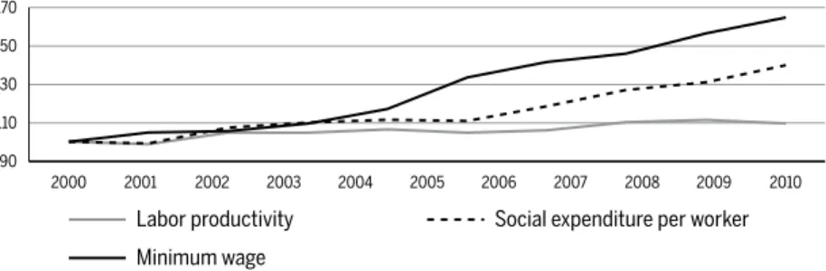
Figure 3 Labor productivity, social expenditure per worker, and minimum wage, 2000-2009 (indexes 2000 = 100)
Source: World Development Indicators, World Bank; CEPALSTAT; Laborstat, ILO, Ipedata.
3 Data from the World DataBank (The World Bank), available at: <http://data.worldbank. org/data-catalog/world-development-indicators>.
-0,6 -0,1
-0,2
-0,3
-0,4
-0,5 0 0,1
Under
valuation inde
x
2000 2001 2002 2003 2004 2005 2006 2007 2008 2009 2010
Labor productivity Social expenditure per worker Minimum wage
90 170
150
130
110
Nevertheless, this period have had its drawbacks. Productivity growth stagnated, while wages and social expenditure rose steadily (see fi gure 3). Moreover, the exchange rate was kept overvalued. The commodities price boom hid Brazilian weaknesses. Asia’s demand guaranteed cur-rent account surpluses, while favorable relative prices for non-tradable goods allowed a boom in the service sector. Growth and employment were kept high, creating a sense of success in economic policy and de-velopment. However, as commodities markets lost momentum, so did Brazil’s growth.
3
Model
This section presents a BOP-constrained model, based on Ribeiro et al. (2016), which illuminates the forces behind the Brazilian path as dis-cussed above. Trade income elasticities are determined by technological gap and income distribution. Government expenditure is included and the difference between those that affect the technological gap and those that affect income distribution is highlighted.
3.1 BOP constraint
We take as a starting point the idea that the long-run rate of growth is that consistent with BOP equilibrium, i.e., the ratio of its income elastic-ity of exports and its income elasticelastic-ity of imports (Thirlwall, 2011). We assume that the world economy consist of two countries: North and South – the South being the laggard economy (in our example, Brazil). For simplicity’s sake, it is assumed that there isn’t capital fl ow between the two economies. Formally, the equations of demand for exports and imports are:
*
P
X A Z
P E
*
P E
M B Y
P
(1)
where X real exports of the South, and M are its real imports. P is the South price level (denominated in Southern currency), while P* is the price level in the North (denominated in Northern currency) and E is the nomi-nal exchange rate (units of Southern currency per unit of Northern cur-rency). Y is the real income of the South and Z is the real income of the North, while η is the price elasticity of exports, ψ is the price elasticity of imports, ε is the income elasticity of exports and π is the income elasticity of imports of consumption goods. A and B are positive constants.
Current account equilibrium requires that:
Substituting equations (1)-(2) into (3), taking logs, differentiating with re-spect to time, and assuming fi xed real exchange rate yields:4
where yBP is the balance-of-payment-constrained growth rate, and z is the
growth rate of the North. As in Ribeiro et al. (2016), we defi ne the trade income elasticities ratio as a function of the technological gap and income distribution:
where T represents the technological gap defi ned as the ratio of the level of the home country’s technological capabilities to the level of the foreign country’s technological capabilities, and σL is the wage share. α1, α2, and
α3 are positive constants.
4 The assumption of fi xed real exchange rate can be questionable, particularly for the Bra-zilian experience. As pointed out by one of the referees, Brazil experienced a steady ap-preciation of its currency in the period 2001-2010, with relevant and negative impacts on its economy (see, for instance, Nassif et al. 2015). A possible extension of the model is to assume that the rate of appreciation of the real exchange rate enters as a component of the balance-of-payment-constrained growth rate. In the simplest case in which the real exchange rate appreciation impacts growth negatively, this new variable would have a positive impact on the intercept of equation (17), so that it would not change the following qualitative results. However, for the sake of tractability and in order to keep focus on the effects of income distribution and technological change on growth, the real exchange rate is assumed constant.
*
P EM PX (3)
BP
z y
(4)
1 2 3
L T
The impact of income distribution on the trade income elasticities ratio can be either positive or negative. In terms of income elasticity of im-ports, as wage share rises, the demand for luxury goods by capitalists falls, while workers’ demand for luxury goods increases, so the magnitude of each case will indicate the net effect. The literature (e.g., Bohman; Nilsson, 2007; Dalgin et al., 2008) emphasizes that, given non-homothetic prefer-ences, more equal economies tend to import less luxury goods, which would give a negative impact of the wage share on the income elasticity of imports.5 However, Souto (2015) suggests that during the commodities price boom the income elasticity of imports increased in Brazil and, more importantly, this rise was stronger for the lowest deciles of income distri-bution. In fact, luxury goods were not the only responsible for the rise of imports. Souto (2015) shows that imports of clothes and furniture, among others, increased during the period.
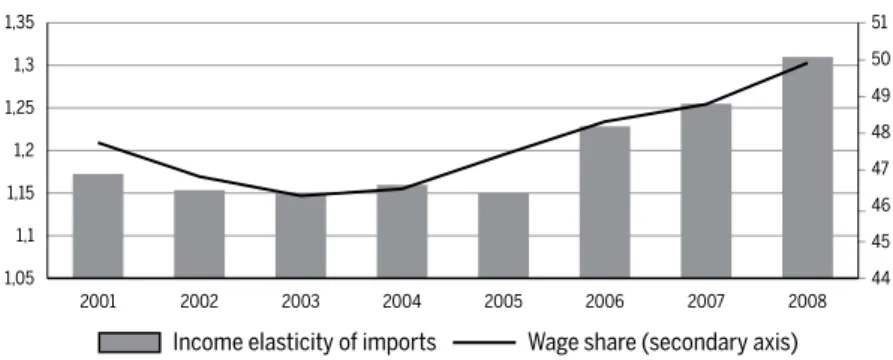
To reassess this analysis, we estimated the income elasticity of imports for Brazil (fi gure 4). We used the bounds testing procedure developed by Pesaran et al. (2001) within an Autoregressive Distributed Lags (ARDL) framework. Later, so as to have different coeffi cients, we used rolling re-gressions, with a constant period of 40 years (see Appendix A for details on the estimation).
Figure 4 Income elasticity of imports and wage share: Brazil, 2001-2008
Note: Wage share was measured using factor costs.
Source: Income elasticity: Authors’ calculation; Wage Share: CEPAL and IBGE
5 Structuralist authors argue (see Furtado (1969), for example, and Ribeiro et al. (2016) for a review of this literature) that higher income inequality leads to higher consumption of luxury goods, which in turn rises income elasticity of imports.
Income elasticity of imports Wage share (secondary axis)
1,05 1,25
1,2
1,15
1,1 1,35
1,3
44 48
47
46
45 50 51
49
2005
Our estimations indicate that the income elasticity of imports rose during the period, which reinforces our assumption. Interestingly, this rise goes along with a rise in the wage share. These results are more likely related to the ris-ing purchasris-ing power of the poor.6 As many families entered the market, the demand for basic goods, such as clothes, wasn’t accompanied by the local in-dustry supply, so that imports rose even for products that are not technology-intensive. Theoretically, several aspects may have infl uenced this result, such as overvalued exchange rate, rising wages, and a weak productive structure. Overvalued exchange rate and rising costs affect external price competitive-ness, while increasing the demand for imported goods. In the meantime, a less diversifi ed structure increases the share of imported goods.
On the other hand, the effect of a rise in the wage share on the income elasticity of exports is less clear. A fall in wage share due to rising labor productivity can lead to specialization in technology intensive goods, which usually present higher income elasticity of exports (see Gouvêa; Lima, 2010). However, if a fall in the wage share is a result of falling wages, an economy can rise its specialization in labor-intensive industries, which have lower income elasticity of exports.
The inverse effect is less clear, as a rise in the wage share due to rising wages won’t necessarily lead to a rise in the specialization of technology intensive goods. Porcile et al. (2007) argue that a rise in wages can improve workers’ capacity to learn, imitate, and improve from foreign technolo-gies, so that a rise in the wage share could lead to specialization in goods with higher income elasticity of exports. This idea is based on three as-sumptions: (1) labor productivity is related to workers’ level of consump-tion (see Basu, 1984; Ray, 1998); (2) higher wages lead to better access to education (see Ranis; Stewart, 2002); (3) higher wages are associated to more effort at work, as suggested by the literature on effi ciency wages (see Shapiro; Stiglitz, 1989). However, as presented above, labor productivity growth in Brazil has been meager, even after a relevant rise in minimum wages, and specialization increased towards primary goods, which most likely affected negatively the income elasticity of exports.
Therefore, the most probable impact of a rising wage share in Brazil was a rise in unit labor costs, without an impact on labor productivity.
Hence, as Souto (2015) and our estimations suggest, income elasticity of imports increased, and the effect over income elasticity of exports was most likely negative. In the present work it is assumed that the impact of a
rise in the wage share on income elasticities is negative .7 Meanwhile, the impact of the technological gap is straightforward. Coun-tries that are closer to the technological frontier are more diversifi ed, with a large share of technology intensive products. This view is strongly support-ed by empirical evidence, as in Fageberg (1988), Verspagen (1993) and Rein-ert (1995). More recently, Gouvêa and Lima (2010) present evidence that more technology intensive sectors have higher income elasticity of exports. Romero and McCombie (2016a) present evidence that more backwards economies have higher income elasticities of demand for high-tech goods than advanced economies. Moreover, Romero and McCombie (2016b) es-timate an expanded Thirlwall’s Law that incorporates non-price competi-tiveness factors, measured by the relative productivity growth. As the in-troduction of this variable affected the elasticities, the estimations suggest that they are endogenous to the relative productivity. All in all, the smaller the technological gap, the higher the income elasticities ratio and, thus, the higher the long-run rate of growth that is consistent with BOP equilibrium.
3.2 Technological gap and income distribution
There are three types of agents in the economy – capitalists, workers, and government. We assume that government levies a tax on profi ts at the rate
τ and spends a share δ in distributive programs and a share (1 – δ ) in public investment, so that the rest of the total income is divided between capital-ists and workers. Formally, total income before tax can be expressed as:
where W are total real wages and ∏ are total profi ts. The government’s budget constraint is given by:
where D are distributive expenditures and I is the fl ow of public invest-ment, so that D = δτ ∏ and I = (1 – δ )τ ∏. Substituting equation (7) into (6), and defi ning distributive expenditures and the fl ow of public investment as a function of profi ts, and normalizing it by the total income (Y), the after tax wage share can be defi ned as:
where σK is the profi t share, and .
As in Ribeiro et al. (2016), we assume that the rate of change of the inverse of the technological gap is a function of the wage share and the inverse of the technological gap itself. Moreover, we stress the impact of public investment on technological progress. Formally:
where β1,β2,β3,β4 and β5 are positive constants. As in Cimoli and Porcile (2014), a lower gap reduces the opportunities of imitation and catching up, so the higher the gap, the higher its rate of change (see also Narula, 2004). As in Lima (2004), technological innovation is determined by distribution in a non-linear way. When the profi t (wage) share is low (high) (assuming that innovation is fi nanced only by profi ts), fi rms aim at investing, but fall short in terms of resources. On the other hand, when profi t (wage) share is high (low), fi rms have suffi cient resources to invest, but the incentives to invest are low (for an empirical analysis, see Aghion et al., 2005). Finally, (6)
Y W
(7)
D I
1 1
Lat Kat K
(8)
L at
W D
Y
K at
1
Y
(9)
2
1 2 3 4 5
L L /
following Cimoli et al. (2015), we assume that public investment has a pos-itive impact on technological capabilities. Public investment that supports innovation and diffusion of technologies is central for catching-up. Public investment increases the quality of infrastructure and education, fi nances basic R&D, and improves the quality of other essential institutions. More-over, as stressed by Mazzucato (2013), the public sector not only fi nances basic R&D, but also plays a key role in the development and diffusion of new technologies as an entrepreneur. All in all, public investment is an important variable for the velocity with which a developing economy is able to reduce the technological gap.
Moreover, note that equation (9) does not explicitly take into account a negative effect of taxation on fi rms’ decision to invest. For simplicity’s sake, we assume that the positive impact of public investment is always higher than the negative effect of taxation, so that we can avoid an additional term in equation (9). In other words, if assumed that fi rms’ investment is a quadratic function of taxation (τ ), we assume herein that any change in taxation takes place with τ remaining to the left of a given maximum value. This assumption does not change the following qualitative results, though.
On the other hand, wage share is determined through a bargain process, where workers set a desired wage. In many developing countries there are well organized unions with considerable bargaining power, which demands a higher wage share in response to a rise in production and labor demand. Even when there is a signifi cant labor surplus in the economy, segmented labor markets allow unions to demand higher wage (for an empirical esti-mation for the wage curve in Brazil, see Barufi et al., 2016). Formally:
where θ is a positive adjustment parameter and is the desired wage share, which is defi ned endogenously as a result of variations in the rate of employment and the ratio of public expenditure in distributive programs and total income:
where γ0,γ1,γ2 and γ3 are positive constants, l is the rate of change of em-ployment and n is the workers’ growth rate (exogenously determined).
(10)
E L
(11)
0 1 / 2
E
L D Y l n
For simplicity’s sake and in order to focus on the effect of distributive programs, we assume that the government affects the desired wage share through its distributive expenditure, which is defi ned exclusively as spend-ing with pensions.8 We assume that the Southern economy counts on the same pension laws as in Brazil, where the minimum pension is the same as the minimum wage, so that a rise in the latter has a direct impact on government expenditure. A rise in the minimum wage can be formally interpreted as a rise in δ -- assuming a constant tax rate. As the minimum wage defi nes a fl oor for workers’ demand, it has a positive impact on the desired wage share. In other words, once the government raises the mini-mum wage, it will be choosing to increase its expenses (social expendi-ture) and, in turn, rising wages on average.
It could be argued that a higher fl ow of public investment raises la-bor productivity, which in turn may have a negative impact on the wage share. However, as presented above, labor productivity growth in Brazil was stagnant, which may indicate that this effect was null. However, even if a negative impact of public investment on the wage share due to a rise in labor productivity is assumed, the following qualitative results would only change if this impact surpasses the positive impact of distributive pro-grams. For the sake of simplicity we abstain from considering such effect. The rate of change of employment is determined as the difference be-tween growth and labor productivity growth. Formally:
where â is the rate of change of labor productivity. Assuming that labor productivity is positively related to growth (Verdoorn’s law), we have:
where a0 is autonomous productivity growth rate and λ is a positive con-stant. Equation (12) can then be rewritten as:
8 Other distributive programs, such as cash transfer programs, were key to reduce income inequality in Brazil (see, for example, Campelo; Neri,2013).
(12)
(13)
(14) lyBPaˆ
0
ˆ
ayBP a
03.3 Equilibrium
Equations (9) and (10) form a two-dimensional system of autonomous differen-tial equations. Defi ning the fl ow of public investment as a function of the wage share in equation (9) and substituting equation (11) (10), and then equations (12)-(14), we fi nd an expanded form of equations (9) and (10), as shown below:
In equation (15), a rise in distributive expenditure by the government rais-es the drais-esired wage (fi rst term in the right-hand side) and, then, raisrais-es the rate of change of the wage share. On the other hand, an increase in the wage share has a negative impact on its rate of change for two reasons: (1) fi rst, as it reduces the growth rate (see equation 5, considering that the sign of α2 is negative), it also reduces the labor demand; (2) second, as the wage share rises, workers’ pressure for higher wages is reduced. In equilibrium ( ), equation (15) yields the following equilibrium:
where
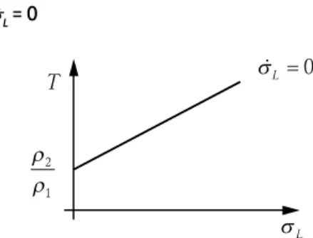
. Assuming, without loss of generality, a suffi ciently high autonomous productivity growth rate and workers growth rate, ρ2 is most likely positive. Figure 5 presents :
Figure 5 The locus σL = 0
(16)
2
1 2 3 4 5
L L 1 1 L
T T
(17)
3 2
1 1
L
T
1 2 3 2 2 0 1 0 1 3
1 z ; a n 1 z ; 1
1 2 2
. 1 z
.
(15)
2 1 2 3 0
1 L T z a n L
ρ ρ
2
1
T σL=0
σL
σL =θ γ
{
0+γ δτ1(
1−σL)
+}
σL=0
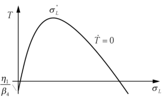
Similarly, setting T = 0 (per equation 16), we fi nd the following equilibrium:
where η1 = β1 + β5 (1 – δ )τ < 0; η2 = β2 – β5 (1 – δ )τ > 0 . It is assumed that the autonomous growth of technological progress is lower in the South than in the North, so that β1 < 0 (it is also assumed that β1 > β5 (1 – δ )τ without loss of generality). Appendix B presents the conditions that guarantee that the roots of equation (18) are within a meaningful domain i.e. and ∈ (0,1) and T (σ *)∈ (0,1). Figure 6 presents T = 0, where is the maximum point of equation (18):
Figure 6 The locus T = 0
Taking the difference between equations (17) and (18) yields:
where . As η2 is assumed negative,
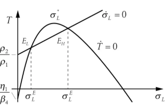
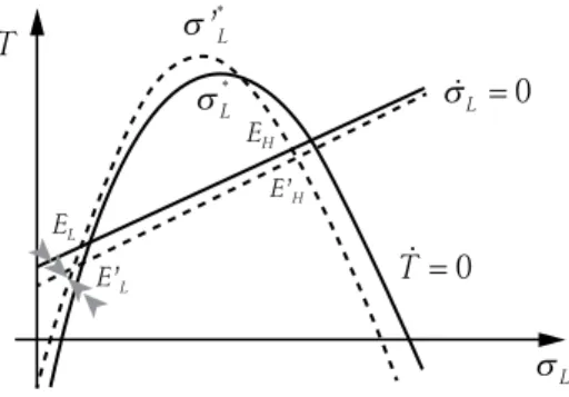
C is unquestionably positive. Assuming that E (T ) has two different real roots (B2 > 4AC ) in the meaningful domain (0, 1), Figure 7 presents the phase-di-agram with its steady states represented by equilibrium points EL (relatively
low growth equilibrium) and EH (relatively high growth equilibrium). EL is an equilibrium of relatively low growth, as it is assumed that α3 is higher than
α2, so that the technological gap is the most important parameter to explain the trade income elasticities.9 Therefore, even though equilibrium E
H has a
9 Whether α3 + α2 is positive or negative is an empirical matter which has not been tested yet. The present model can easily represent both scenarios. However, without loss of
gener-.
2
1 2 3
4 4 4
L L
T
(18)
1
L
2
L
. *
L .
2L L
E T A B C (19)
3
2 4 1 1 3 4 2 1
4
; ;
A B C
T =0
η β 1
4
σL*
T
smaller technological gap (higher T ), but also a higher wage share (higher σL ), the net effect in terms of growth is positive (higher trade income elasticities).
Figure 7 The loci T = 0 and σL
In order to analyze the stability conditions of equilibrium points EL and EH, we derive (assuming θ = 1 without loss of generality) the Jacobian matrix of the system formed by equations (15) and (16):
The trace of the Jacobian is negative, but the sign of the determinant de-pends on the interaction between the wage share and the technological gap. More precisely, it depends on the equilibrium wage share ( ). If the equilibrium point is at the left side of the maximum point, so that is more likely to be positive, the determinant is more likely to be negative (saddle point).10 On the other hand, if the equilib-rium point is at the right side of the maximum point, so that is more likely to be negative, the determinant is more likely posi-tive and the system stable. Therefore, under some assumptions, equilibrium point EL is assumed unstable and equilibrium point EH is assumed stable.
ality, we assume that α3 > α2.
10 In order to , it is assumed, without loss of generality, that the tax rate is suffi ciently small, so that the determinant is negative and the system unstable. Moreover, it is assumed that , so that the determinant is positive and the system stable.
E L
2 2 3 5 1
E L
2 2 3
E L
5 1 12 2 3 5 1 E L
2 2 2 3 5 1
E L . . ρ ρ 2 1 η β 1 4
T σL=0
σL E
EL EH
σL
E σ
L
T =0
σL * J dT dT dT d d dT d d L L L L L E = = − − −
(
−)
−(
)
ɺ ɺ σ σ σ σβ β β σ β δ τ
γ λ α
4 2 3 5
2
2 1
4
Distributive policy
Suppose the Southern economy opts for intensifying its distributive ex-penditures, so that it raises the minimum wage. This rise has a direct impact on total expenditures, with two possible outcomes: (1) fi rst, the government can raise the tax rate and fi nance distributive expenditures without harming public investment; (2) second, the government raises dis-tributive expenditures at the expense of public investment. In this section, we focus on the case where the tax rate is kept constant and the govern-ment chooses to give more importance to social expenditures.
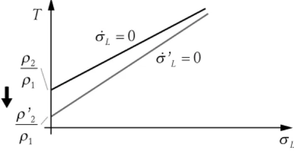
Formally, the South rises δ. The solid line in Figure 8 presents σL = 0, while
the dotted line represents the effect of a rise in distributive expenditures:
Figure 8 The impact of a rise in distributive expenditures on locus σL = 0
Per equation (17), a rise in δ reduces ρ2, which in turn reduces the intercept of σL = 0. Moreover, a rise in δ increases ρ3, with a positive effect on the slope of σL = 0 (see fi gure 4). On the other hand, per equation (18), a rise in
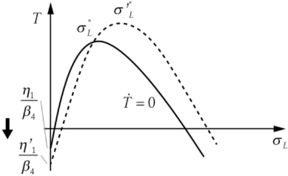
δ decreases η1, which in turn reduces the intercept of T = 0 (see Figure 9). Moreover, a rise in δ increases the point of maximum and increases both real roots (see Appendix C).
Figure 10 presents the phase diagram, with the dotted lines represent-ing the effect of a rise in δ. First, supposing that the Southern economy is placed in the equilibrium EL (a saddle path equilibrium), a rise in δ moves the equilibrium slightly to the Southeast, so that the equilibrium EL is placed at the left of the saddle path of the new equilibrium point E’L. Only
when the equilibrium point EL happens to be exactly in the saddle path it
will move towards the new equilibrium point E’L. On the contrary, if the equilibrium point EL happens to be at the left of the new saddle path, the
.
.
. .
.
ρ ρ
2
1
ρ ρ
’2
1
σ’
L=0
T
σL =0
economy is moving towards the left, reducing both T and σL.
On the other hand, equilibrium point EH (a stable equilibrium) moves to the Northeast. As the new equilibrium point E’H is stable, the behavior of
the system pushes the economy towards the new equilibrium, where the technological gap is smaller and the wage share is higher.
Figure 9 The impact of a rise in distributive expenditures on locus T = 0
Figure 10 The impact of a rise in distributive expenditures on the dynamics between T and σL
Firstly, we focus on equilibrium point EL, as it happens to be the case of many developing economies (low wage share and high technological gap). A rise in the wage share harms the technological progress (as it reduces public investment) while intensifying the external constraint. More pre-cisely, the focus on direct redistribution at the expense of public invest-ment may lead to sluggish structural change, less employinvest-ment growth and a weakening of the labor market and labor bargaining power. These re-sults suggest that there is little room for redistributive policies (when not
T=0
η β 1
4
σL
*
T
η β
’1
4
σ’*
L
σL
.
T =0
σL*
T
σL=0
EL
EH
E’L
E’H
σ’*
L
accompanied by technological progress) in developing economies whose production structure is weak.
Lastly, in terms of balance-of-payment-constrained growth rate, note that the new equilibrium point E’L has a relatively higher technological
gap and relatively higher wage share. As stated by equation (5), a fall in T
and a rise in σL lead, considering that the sign of α2 is negative, to a lower trade income elasticities ratio, so that the long-run rate of growth that is consistent with BOP equilibrium is relatively lower.
On the other hand, the new equilibrium point E’H faces a relatively smaller technological gap and a higher wage share, so that the long-run rate of growth is most likely higher. When the technological gap is small and total income is more equally distributed, income distribution has a positive impact on the technological gap, income distribution and, fi nally, on growth consistent with the BOP equilibrium.
4.1 A rise in the tax rate (a combination of both policies)
In this section we take a step forward and explore a situation where both social expenditure and public investment are prioritized. Instead of choos-ing one type of expenditure, the government opts for increaschoos-ing both kinds of expenditures through a rise in the tax rate. Formally, we take the case of a rise in the tax rate (τ ), without changes in the share of each type of expenditure11. By equation (17), a rise in τ decreases ρ
2 and increases ρ3, with a negative impact on the intercept and a positive effect on the slope of σL = 0.
By equation (18), a rise in τ increases η1, which in turn raises the intercept of T = 0. Moreover, a rise in τ reduces the point of maximum and reduces both real roots (see Appendix C). Figure 11 presents the effect of a rise in the tax rate, where the dotted lines represent the new isoclines. A rise in τ pushes both equilibrium points to the Southwest. Consider an economy placed in the equilibrium point EL. Note that differently from the previous case, the equilibrium point EL happens to be to the right of the new saddle
11 For the sake of simplicity, we don’t discuss the impact of taxation on profi ts and wages and the way its impact fi rms’ decisions and consumption behavior. Conceptually, we assume that government expenditure lies in a region where it is more productive than fi rms’ invest-ment. It is assumed that taxation is still very small and that changes in taxation are more favorable than harmful to the economy.
path, so that the system’s behavior pushes the economy to the right – to the new equilibrium E’H.
Figure 11 The impact of a rise in the tax rate
Conceptually, distributive expenditure and technological catching-up go hand in hand, allowing a virtuous cycle of growth and income distribu-tion. As a result, the new equilibrium point E’H attains a higher T and σL in comparison to the initial equilibrium EL, with the impact on the income elasticities depending on the parameters of the model. As earlier assumed that the impact of the technological gap on the income elasticities is higher than the negative impact of a rise in the wage share, the most likely out-come of both is a higher ratio of inout-come elasticities, so that the long-run growth consistent with BOP equilibrium is higher. All in all, when the technological gap happens to be small and total income is poorly distrib-uted, a combination of income distribution and productive public invest-ment has a positive impact on the technological gap, income distribution and, fi nally, on growth consistent with BOP equilibrium.
5
Conclusion
This paper discusses, in a BOP dominated macrodynamic model, the im-pact of distributive policies and public investment on the BOP-constrained rate of growth. We take the Brazilian economy, in the context of the com-modities boom, as a background for our theoretical model.
It is suggested that distributive programs can harm long-term growth, as it harms the technological progress while intensifying the external
con-σL
T=0
σL*
T
σL=0
EL
EH
E’L
E’H
σ’*
straint. In other words, direct redistribution at the expense of public in-vestment may lead to sluggish structural change, less employment growth and a weakening of the labor market and labor bargaining power, so that the economy moves towards complement underdevelopment.
Lastly, it is argued that the right balance of public investment and dis-tributive programs would allow a virtuous cycle of growth and income distribution to emerge. A rise in public investment reduces the techno-logical gap, while a rise in distributive expenses causes a more egalitarian distribution. Moreover, the combination of these policies leads to a higher long-run growth.
References
AGHION, P.; BLOOM, N.; BLUNDELL, R., GRIFFITH, R.; HOWITT, P. Competition and In-novation: An Inverted-U Relationship. The Quarterly Journal of Economics, v.120, n.2, p.701-728, 2005.
BARUFI, A.; HADDAD, E.; NIJKAMP, P. New evidence on the wage curve: Non-linearities, urban size, and the spatial scale in Brazil. Proceeding of the 44th Brazilian Economic Meeting, ANPEC. Brazilian Association of Graduate Programs in Economics, 2016. Available at <www.anpec.org.br/encontro/2016/submissao/fi les_I/i10-b94c515cd9ff9f074c7db2ece-d6acadd.pdf>. Accessed in 09/01/2016.
BASU, K. The Less Developed Economy: A Critique of Contemporary Theory. Oxford: Basil Blackwell, 1984.
BHADURI, A.; MARGLIN, S.A. Unemployment and the real wage: the economic basis for contesting political ideologies. Cambridge Journal of Economics, v.14, n.4, p.375-393, 1990. BLECKER, R. A. International Competition, Income Distribution and Economic Growth.
Cambridge Journal of Economics, v.13, n.3, p.395-412, 1989.
BOHMAN, H.; NILSSON, D. Income inequality as a determinant of trade fl ows. International Journal of Applied Economics, v.4, n.1, March, p.40-59, 2007.
CAMPELO, T.; NERI, M. (Ed.). Programa Bolsa Família: uma década de inclusão e cidadania. Brasília: IPEA, 2013.
CARVALHO, L.; RUGITSKY, F. Growth and Distribution in Brazil in the 21st Century: Re-visiting the Wage-Led Versus Profi t-Led Debate. Department of Economics FEA/USP Working Paper Series n. 2015-25, 2015.
CIMOLI, M.; PORCILE, G. Technology, structural change and BOP-constrained growth: a structuralist toolbox. Cambridge Journal of Economics, v.38, n.1, p.215-237, 2014.
DALGIN, M.; TRINDADE, V.; MITRA, D. Inequality, Nonhomothetic Preferences, and Trade: A Gravity Approach. Southern Economic Journal, v.74, n.3, p.747-774, 2008.
DUTT, A. K. Stagnation, income distribution and monopoly power. Cambridge Journal of Eco-nomics, v.8, p.25-40, 1984.
ECLAC. Horizons 2030: Equality at the centre of sustainable development. Santiago: ECLAC, 2016.
FAGERBERG, J. International competitiveness. The Economic Journal, v.98, p.355-374, 1988. FURTADO, C. Um projeto para o Brasil. Rio de Janeiro: Saga, 1969.
GOUVEA, R. R.; LIMA, G. T. Structural change, balance-of-payments constraint, and eco-nomic growth: evidence from the multisectoral Thirlwall’s law. Journal of Post Keynesian Economics, v.33, n.1, p.169-204, 2010.
GOUVEA, R. R.; LIMA, G. T. Balance-of-payments-constrained growth in a multisectoral framework: A panel data investigation. Journal of Economic Studies, v.40, n.2, p.240-254, 2013.
LIMA, G. T. Endogenous technological innovation, capital accumulation and distributional dynamics. Metroeconomica, v.55, n.4, p.386-408, 2004.
MAZZUCATO, M. The Entrepreneurial State: Debunking the Public vs. Private Myth in Risk and Innovation. London: Anthem, 2013.
NARULA, R. Understanding Absorptive Capacities in an Innovation Systems Context: Con-sequences for Economic and Employment Growth. DRUID Working Paper no. 04-02, 2004. NASSIF, A.; FEIJO, C.; ARAUJO, E. Overvaluation trend of the Brazilian currency in the
2000s: empirical estimation. Revista de Economia Política, v.35, n.1, p.3-27, 2015.
OREIRO, J. L.; PUNZO, L. F.; ARAUJO, E. Macroeconomic constraints to growth of the Bra-zilian Economy: diagnosis and some policy proposals. Cambridge Journal of Economics, v.36, n.4, p.919-939, 2012.
PESARAN, M. H.; SHIN, Y.; SMITH, R. J. Bounds Testing Approaches to the Analysis of Level Relationships. Journal of Applied Econometrics, v.16, n.3, p.289- 326, 2001.
PORCILE, G.; DUTRA, M. V.; MEIRELLES, A. J. A. Technological gap, real wages, and learn-ing in a balance-of-payments-constrained growth model. Journal of Post Keynesian Econom-ics, v.29, n.3, p.473-500, 2007.
RANIS, G.; STEWART, F. Crecimiento Económico y Desarrollo Humano en América Latina. Revista de la CEPAL, v.78, p.8-18, 2002.
RAY, D. Development Economics. Princeton: Princeton University Press, 1998.
REINERT, E. S. Competitiveness and its predecessors - a 500 year cross-national perspective. Structural Change and Economic Dynamics, v.6, p.23-42, 1995.
RIBEIRO, R. S. M.; MCCOMBIE, J. S. L.; LIMA, G. T. Exchange Rate, Income Distribution and Technical Change in a Balance-of-Payments Constrained Growth Model. Review of Political Economy, v. 28, p.545-565, 2016.
ROMERO, J. P.; MCCOMBIE, J. S. L. The Multi-Sectoral Thirlwall’s Law: Evidence from 14 Developed European Countries using Product-Level Data. International Review of Applied Economics, v.30, n.3, p.301-25, 2016a.
ROMERO, J. P.; MCCOMBIE, J. S. L. Thirlwall’s Law and the Specifi cation of Export and Im-port Demand Functions: An Investigation of the Impact of Relative Productivity Growth on Trade Performance. CCEPP WP02-16, Cambridge Centre for Economic and Public Policy. 2016b.
SERRANO, F.; SUMMA, R. Macroeconomic policy, growth and income distribution in the Brazilian Economy in the 2000s. Investigación Económica, v. 71, n. 282, p. 55-92, 2012. SHAPIRO, C.; STIGLITZ, J. Equilibrium Unemployment as a Worker Discipline Device.
American Economic Review, v.74, n.3, p.433-444, 1989.
SOUTO, A. M. Distribuição pessoal da renda e elasticidade renda da demanda por importações no Brasil: evidências a partir de regressões quantílicas para o período 2002-2009. 2015. Master’s Dissertation – University of São Paulo, São Paulo, 2015. Available at <http:// www.teses.usp.br/teses/disponiveis/12/12138/tde-22022016 153505/>. Accessed in 07/03/2016.
THIRWALL, A. P. Balance-of-payments constrained growth models: history and overview. PSL Quartely Review, v.64, n.259, p.307-351, 2011.
TIMMER, M. P.; DIETZENBACHER, E.; LOS, B.; STEHRER, R.; DE VIRES, G. J. An Illus-trated User Guide to the World Input–Output Database: the Case of Global Automotive Production. Review of International Economics, v.23, p.575–605, 2015.
VERSPAGEN, B. Uneven Growth between Interdependent Economies. Avebury: Aldershot, 1993.
About the author
Antonio Soares Martins Neto - [email protected]
Economic Commission for Latin America and the Caribbean (ECLAC), Santiago, Chile.
I thank two anonymous referees for useful comments and suggestions. I am also grateful to Rafael Ribeiro and Gabriel Porcile for useful conversations, comments and suggestions. The usual disclaimer applies.
About the article
Appendix
Appendix A
The empirical estimation of income elasticity of imports for Brazil is based on the estimation of the following aggregate import demand function:
where M, R and Y are imports, real exchange rate, and domestic GDP respectively. The sample period covers annual data from 1962 to 2014. GDP data in constant 2000 US$ dollars was obtained from the World De-velopment Indicators (WDI). The real exchange rate is constructed as the nominal exchange rate for each country multiplied by the ratio between the wholesale price index of US and consumer price index for each coun-try. The real exchange was gathered using data from the International Fi-nancial Statistics of the International Monetary Fund. The trade data have been collected from the United Nations Commodity Trade Statistics Da-tabase (COMTRADE) according to the Standard International Trade Clas-sifi cation (SITC) Revision 1. Following Gouvea and Lima (2013), the trade data was defl ated using the US GDP defl ator from WDI.
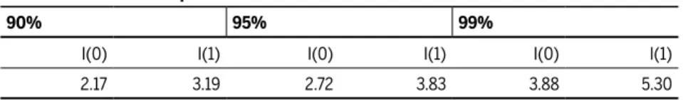
First, we need to verify the existence of a cointegration relationship among these variables. The bounds testing procedure developed by Pesaran et al. (2001) was used within an Autoregressive Distributed Lags (ARDL) framework. The results of our test for a long-run relationship (cointegration) is presented below:
Table A1 Cointegration test
Critical value bounds of the F-statistic: intercept and no trend
H0: no levels relationship
90% 95% 99%
I(0) I(1) I(0) I(1) I(0) I(1)
2.17 3.19 2.72 3.83 3.88 5.30
Calculated F-statistic.
F = 9.404.
t
t
tNote that the computed F-statistic exceeds the critical values at 99% confi dence level. As a cointegration relationship is verifi ed, we can estimate the coeffi cients. An ARDL (1,0,2) specifi cation is used, so that we have:
Table A2 Long-run relationship
Regressors Coeffi cients
Import demand
Yt *** 1.174
RT *** -1.549
Note that both coeffi cients are signifi cant at 99% and have the expected sign. In order to have different coeffi cients for the period, a rolling window was used. The sample size is constant over time to maintain the statistical power and was set as 40 observations (i.e, our fi rst estimation is from 1962 to 2001). The results are presented in Figure 4.
Appendix B
Per equation (18), setting E(T) equal to zero, we obtain:
As η1 is negative, the condition for us to have two real roots is (∆ > 0):
Assuming that this condition is fulfi lled, the conditions with respect to the domain of both roots were analyzed.
Second root
Per equation (18), we have that:
2
3 L 2 L 1 0
2
2 3 1
4
2
2 3 1
2 2
3 3
4
2 2
L
(B.1)
(B.2)
As we obtain:
Condition (1), :
Since all parameters are positive, . Condition (1), :
Since η1 < 0, the condition will be fulfi lled if β3 – 2η2 ≥ 0. As η2 = β2 – β5 (1 – δ )τ, this condition is true if β3 > 2β2 or the tax rate is suffi ciently small and β5 is suffi ciently large. We assume hereafter that one of these conditions are satisfi ed, so that < 1.
First root
Per equation (18), we have that:
2
2 3 1
2 * 3 4 2 L 2 0 L (B.4) (B.5) (B.6) (B.7) (B.8) 2
2 3 1
* 3 4 0 2 2 0 L 2 1 L 2
2 3 1
* 3 4 1 2 2
2 2 4 3 1 2 3
2
3 1 3 3 2
4 2 4
1 3 2
2 2
2
L
2
2 3 1
1 2 3 3 4 2 2 L 2
2 3 1
1 * 3 4 2 L
* 2 2
Condition (1), :
As η1 < 0, the fi rst condition is fulfi lled, so that . Condition (1), :
As , so it is also .
In terms of T(σ *), the conditions for T(σ *) ∈ (0, 1) are:
The conditions are most likely to hold if β3 is suffi ciently smaller than 2, so that T(σ *) > 0. Moreover, as we expect [ β2 – β5 (1 – δ )τ ]² to be small, given our earlier assumption, T(σ *) is expected to be smaller than 1. Our follow-ing analysis will assume that these conditions hold.
1 0 L (B.9) (B.10) (B.11) 2
2 2 4 3 1
2 2
2 2 4 3 1
1 0 L 2
2 3 1
* 3 4 1 2 1 1 L 2 1 L
1
1 L
* *2
1 2 3
4 4 4
0 L L 1
2 2
1 2 2
4 3 4 4
0 1 2 4
1 5 2 5 2 5
4 4 3 4
1 [ 1 ]² [ 1 ]²
1 4 2 2
2 3 1
Appendix C
Per equation (18), we have that:
where η2 = β2 – β5 (1 – δ )τ. Therefore, we obtain:
With respect to the real roots, recall that:
Since and are negligible, we obtain:
* 5 0
*5 1 0
2
2 3 1
1 * 3 4 2 L 2
2 3 1
2 * 3 4 2 L (C.2) (C.4) (C.6) (C.3) (C.5) (C.7) 1 2 0; 0 L L 1 2 0; 0 L L 2
2 3 1
3 4 2 2
2 3 1