1
UAV - based imagery processing using Structure from
Motion and Remote Sensing technology
i
UAV - based imagery processing using Structure from Motion
and Remote Sensing technology
Supervised by
Gabriel Ignacio Guerrero Castex, PhD
Institute of New Imaging Technologies, Universitat Jaume I, Castellón de la Plana, Spain
Co-supervised by Torsten Prinz, PhD
Institut für Geoinformatik, Westfälische Wilhelms-Universität, Münster, Germany
Co-supervised by Mário Caetano, PhD
Instituto Superior de Estatística e Gestão de Informação, Universidade Nova de Lisboa,
Lisbon, Portugal
ii
ACKNOWLEDGEMENTS
I would like to thank my supervisor Dr. Guerrero for his advices, patience, time and effort he dedicated to my thesis. Next, I would like to thank the co-supervisors, Dr. Prinz for his comments and suggestions as well as to Dr. Caetano for his advices and comments.
I would like to thank to M.Sc. Jan Lehmann for providing me an opportunity to work with his data as well as for the advices, comments and spent time.
Also I would like to express my thankfulness to the European Commission and Erasmus Mundus Master in Geospatial Technologies for providing me the opportunity to study this study program.
iii
UAV - based imagery processing using Structure from
Motion and Remote Sensing technology
ABSTRACT
iv
KEYWORDS
Structure from Motion Unmanned Aerial Vehicle Unmanned Aerial System DSM
v
ACRONYMS
API Application Programming Interface
BBA Bundle Block Adjustment
BNDVI Blue Normalized Difference Vegetation Index CMVS Clustering views for Multi-View Stereo
CIR Color Infrared
CPU Central Processing Unit
CUDA Compute Unified Device Architecture
DEM Digital Elevation Model
DGPS Differential GPS
DSM Digital Surface Model
EO External Orientation
GCP Ground Control Points
GCS Ground Control Station
GLSL OpenGL Shading Language
GPS Global Positioning System
GPU Graphics Processing Unit
IDW Inverse Distance Weighted
IHS Intensity Hue Saturation
IMU Inertial Measurement Unit
INSPECTED.NET INvasive SPecies Evaluation, ConTrol & EDucation.NET
IO Internal Orientation
MSL Mean Sea Level
NDVI Normalized Difference Vegetation Index
NIR Near Infrared
NN1 Nearest Neighbor 1
NN2 Nearest Neighbor 2
OBIA Object Oriented Image Analysis OpenCL Computing Language
OpenGL Open Graphics Library
vi
PMVS2 Patch-based Multi-View Stereo
RBMC Brazilian Network for Continuous Monitoring of the GNSS Systems in real time
RGB Red Green Blue
RMSE Root Mean Square Error
S1 Segment 1
S2 Segment 2
SfM Structure from Motion
SIFT Scale Invariant Feature Transform
UA Unmanned Aircraft
UAS Unmanned Aerial System
UAV Unmanned Aerial Vehicle
UTM Universal Transverse Mercator
VTOL Vertical Take-Off and Landing
vii
INDEX OF THE TEXT
ACKNOWLEDGEMENTS ... ii
ABSTRACT ... iii
KEYWORDS ... iv
ACRONYMS ... v
INDEX OF THE TEXT ... vii
INDEX OF TABLES ... x
INDEX OF IMAGES ... xi
INDEX OF FORMULAS ... xiii
1 Introduction ... 1
1.1 Problem statement and objectives ... 2
1.2 Text organization ... 3
2 Background ... 4
2.1 UAS in Remote Sensing applications ... 4
2.2 Traditional Methods ... 5
2.3 Structure from Motion ... 6
2.3.1 Scale Invariant Feature Transform ... 7
2.3.2 Bundle Block Adjustment ... 7
2.3.3 CMVS and PMVS2 ... 8
2.4 GPU-based processing ... 9
2.4.1 CUDA ... 11
2.4.2 OpenCL ... 11
2.4.3 OpenGL and GLSL ... 11
2.5 Software implementations of SfM ... 12
2.5.1 PhotoScan ... 12
2.5.2 VisualSfM ... 13
2.6 Image enhancements ... 15
2.6.1 Vegetation indices ... 15
2.6.2 IHS transformation ... 16
2.7 Surface elevation extraction ... 18
2.8 Object Oriented Image Analysis ... 19
viii
2.8.2 Classification in eCognition ... 21
2.8.3 OBIA and UAV data... 21
3 Resources ... 22
3.1 Study area ... 22
3.2 Materials ... 23
3.2.1 Platform ... 23
3.2.2 Imagery and cameras ... 24
3.2.3 GPS data ... 25
4 Implementation ... 26
4.1 Data preparation ... 26
4.1.1 Differential GPS correction ... 26
4.1.2 Image selection ... 26
4.2 Image processing using Agisoft PhotoScan... 27
4.2.1 Feature detection and matching ... 28
4.2.2 Georeferencing and camera optimization ... 31
4.2.3 Point cloud densification ... 31
4.2.4 Mesh reconstruction ... 31
4.3 Image processing using VisualSfM ... 33
4.3.1 Feature detection ... 34
4.3.2 Feature matching ... 36
4.3.3 MaxSIFT parameter ... 36
4.3.4 Sparse cloud reconstruction ... 37
4.3.5 Cloud densification ... 39
4.3.6 Point cloud georeferencing and DSM export ... 39
4.3.7 Orthophoto export and georeferencing ... 40
5 Acacia tree classification ... 41
5.1 Data enhancements ... 41
5.2 Classification schema and spectral behavior ... 42
5.3 Classification using RGB data ... 43
5.3.1 Coarse classification ... 43
5.3.2 Fine classification ... 44
ix
5.4.1 Coarse classification ... 45
5.4.2 Fine Classification ... 46
6 Results and discussion ... 47
6.1 PhotoScan-based workflow results ... 47
6.2 VisualSfM-based workflow results ... 51
6.3 Orthophoto results comparison ... 54
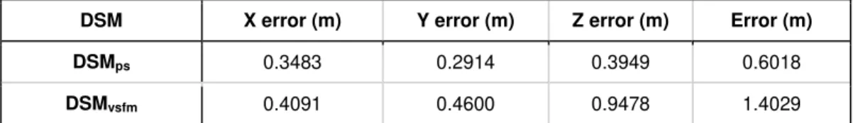
6.4 DSM results comparison ... 55
6.4.1 Georeferencing precision ... 55
6.4.2 Absolute and relative DSM precisions ... 56
6.5 Workflows comparison ... 59
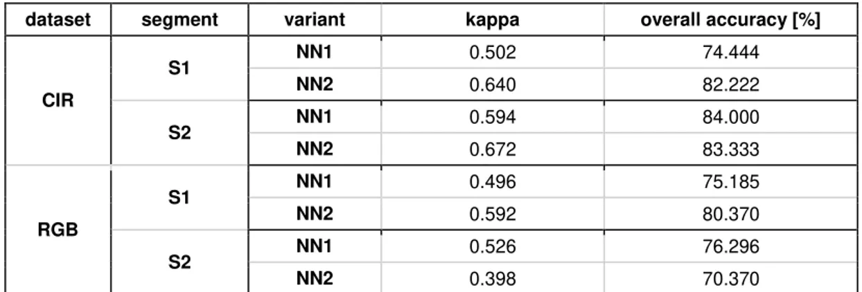
6.6 Classification results ... 61
7 Conclusion ... 64
References ... 65
Appendix A ... 71
x
INDEX OF TABLES
Tab. 1.: Detailed information of acquired imagery ... 24
Tab. 2.: Results of RGB imagery stitching using different variations of parameters using PhotoScan... 29
Tab. 3.: Results of CIR imagery stitching using different variations of parameters using PhotoScan... 30
Tab. 4.: Results of RGB imagery stitching using different variations of parameters in VisualSfM ... 37
Tab. 5.: Results of CIR imagery stitching using different variations of parameters in VisualSfM. ... 37
Tab. 6.: Details of point cloud densification using CMVS/PMVS2. ... 39
Tab. 7.: X.: X, Y, Z and total error of georeferencing the point clouds. ... 55
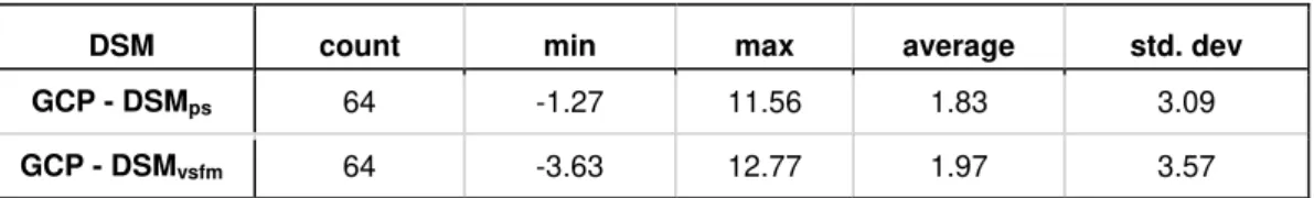
Tab. 8.: Difference statistics of both DSMs. ... 57
Tab. 9.: Summary of obtained results characteristics using different workflows. ... 60
Tab. 10.: Classification accuracies for all classification variants. ... 62
Tab. 11.: Classification and aggregation schema for RGB dataset. ... 74
Tab. 12.: Classification and aggregation schema for CIR dataset. ... 74
Tab. 13.: Results of georeferencing in PhotoScan-based workflow. ... 75
Tab. 14.: Results of georeferencing in VisualSfM-based workflow. ... 75
Tab. 15.: Confusion matrix S1NN1cir. ... 76
Tab. 16.: Confusion matrix S1NN2cir. ... 76
Tab. 17.: Confusion matrix S1NN1rgb. ... 76
Tab. 18.: Confusion matrix S1NN2rgb. ... 76
Tab. 19.: Confusion matrix S2NN1cir. ... 77
Tab. 20.: Confusion matrix S2NN2cir. ... 77
Tab. 21.: Confusion matrix S2NN1rgb ... 77
xi
INDEX OF IMAGES
Img.1.: Example of SfM workflow. Source: WESTOBY et al., 2012. ... 9
Img. 2: History of GPU languages development. Source: BRODTKORB et al., 2013. ... 10
Img. 3.: Spectral behavior of vegetation. Source: JENSEN, 2005. ... 16
Img. 4.: Principles of IHS transformation. Source: LILLESAND et al.,1994;DOBROVOLNY, 1998. ... 17
Img. 5.: Location of study area. ... 22
Img. 6.: Mussununga vegetation structure. Source: SAPORETTI-JUNIOR et al., 2012. ... 23
Img. 7.: DGPS Acacia measurements and location of segments. ... 25
Img. 8.: Workflow diagram of data pre-processing using PhotoScan. ... 28
Img. 9.: Sparse point cloud (a), dense point cloud (b) and mesh (c) created based on RGB imagery. ... 32
Img. 10.: Sparse point cloud (a), dense point cloud (b) and mesh (c) created based on CIR imagery. ... 32
Img. 11.: Schema of VisualSfM-based workflow. ... 34
Img. 12.: Diagram of Surface band extraction workflow. ... 41
Img. 13.: Spectraplot of classes defined in RGB dataset. ... 42
Img. 14.: Spectraplot of classes defined in CIR dataset. ... 43
Img. 15.: Influence of accuracy and point limit parameters on stitching results of CIR dataset... 48
Img. 16.: Influence of accuracy and point limit parameters on stitching results of RGB dataset... 48
Img. 17.: Processing times of each subprocess in RGB imagery stitching with respect to parameter setup. ... 50
Img. 18.: Processing times of each subprocess in CIR imagery stitching with respect to parameter setup. ... 50
Img. 19.: Influence of -TC2 and MaxSIFT parameters on image stitching in RGB dataset processing... 51
xii
Img. 21.: Processing times of each subprocess in RGB imagery stitching with respect to
parameter setup. ... 53
Img. 22.: Processing times of each subprocess in CIR imagery stitching with respect to parameter setup. ... 53
Img. 23.: Orthophotos capturing Segment 1 derived from both datasets. a) PhotoScan-based RGB result; b) VisualSfM-PhotoScan-based RGB result; c) PhotoScan-PhotoScan-based CIR result; d) VisualSfM-based CIR result. ... 54
Img. 24.: Elevation difference between GCP and DSMps. ... 56
Img. 25.: Elevation difference between GCP and DSMvsfm. ... 56
Img. 26.: DSMs created by different workflows; a) DSMps; b) DSMvsfm ... 57
Img. 27.: Difference between DSMps and DSMvsfm. ... 58
Img. 28.: Statistics of DSM differences. ... 58
Img. 29.: Cumulative processing times for both datasets and workflows. ... 59
Img. 30.: Comparisons of variant couples within CIR dataset type and segment. ... 62
Img. 31.: Comparisons of variant couples within RGB dataset type and segment. ... 63
Img. 32: Classification workflow for RGB dataset. ... 71
Img. 33: Classification workflow for CIR dataset. ... 72
xiii
INDEX OF FORMULAS
1
1
Introduction
Technical development and component miniaturization in the recent years allowed a rapid increase in usage of the Unmanned Aerial Systems (UAS) for various application purposes. In the field of Remote Sensing, UAS proved to be a feasible sensor platforms (WATTS et al., 2012; TURNER et. al, 2012; GUPTA et al., 2013). However, in contrast with conventional aerial imagery, UAS-based data posses a set of specific characteristics such as lack or low precision of the External or Internal parameters, high angular or rotational variability etc. (TURNER et al., 2012; ZHANG et al., 2011). Several algorithms developed in the field of computer vision in the recent years have been applied to process UAS data. In order to extract products from the data serving for further analysis, the camera parameters have to be estimated. A set of problems associated with such a goal was solved by multiple algorithms such as Scale Invariant Feature Transform (TURNER et al., 2012). Structure from Motion is a toolchain providing the solution utilizing various algorithms with purpose to detect features on the images, perform their matching and consequently estimate camera parameters (WESTOBY et al., 2012). Being implemented in various software, users have a set of possibilities how to process their UAS data. However, software solutions can vary in the quality of a result or processing time amount. Moreover, several difficulties in the image processing can raise, such as image blur decreasing the quality or small image overlaps. Such situations can occur due to a platform instability caused by external factors (e. g. wind) or deviations from flight plan caused by insufficient precision of an onboard GPS unit (HUNT et al., 2012; TURNER et al., 2012).
2
MUENSTER, 2015). A part of a project proposed by M.Sc. Jan Lehmann (Institute of Landscape Ecology, WWU Muenster, Germany) utilize the Remote Sensing technology. Imagery was collected using UAS technology. In this thesis, data collected by M.Sc. Jan Lehmann within the INSPECTED.NET project will be used in order to present raw image processing workflows and perform results comparison.
1.1
Problem statement and objectives
In order to extract as much information possible from the obtained imagery, raw data have to be processed - images have to be aligned, camera parameters have to be estimated and point clouds generated. Consequently, products such as Digital Surface Model (DSM) and orthophoto can be derived. Such a procedures can be executed using different software and different parameter setup. Finally, quality assessment has to be performed, in order to compare the results quality.
Main objectives of this thesis can be concluded as follows:
presentation of raw UAS imagery processing workflows using different software
estimation of optimal software parameter setup for camera parameters estimation within each workflow
comparison of the resulting products in terms of quality and accuracy
comparison of workflows feasibility with respect to resulting processing time and quality
Secondary objectives then can be concluded as:
demonstration of obtained product usage within Acacia classification
3
1.2
Text organization
4
2
Background
2.1
UAS in Remote Sensing applications
Unmanned Aerial System (UAS) consists of an aircraft, associated sensors and control equipment. The aircraft is not operated by a human operator, whereas it is controlled remotely or flies autonomously (GUPTA et al., 2013). UAS, also referred as UAVs (Unmanned Aerial Vehicles) have long military tradition. However, in 1990 numerous smaller organizations developed efforts, encouraged by technical improvements and miniaturization of components such as GPS (Global Positioning System) or Inertial Measurement Unit (IMU), in order to modify UAS for the research purposes. Vast variety of UAS is available nowadays for a palette of applications (WATTS et al., 2012; TURNER et. al, 2012). UAS became feasible solution for a range of applications such as search and rescue, real-time surveillance, reconnaissance operations, traffic monitoring, hazardous site inspection or agriculture monitoring (GUPTA et al., 2013).
UAS consists of a two main components: the unmanned aircraft (UA) and Ground Control Station (GCS). According to the different characteristics such as aerodynamics or size, it is possible to classify UA as follows (GUPTA et al., 2013):
Fixed-wing UA - unmanned airplane with wings, which requires a take-off and landing runway and flies with high cruising speeds and long endurance.
Rotary-wing UA - also referred as Vertical Take-Off and Landing (VTOL) does not require runway, has ability to hover and flies with high maneuverability. Different hardware configurations (number of motors) are possible (helicopter, coaxial-, tandem- or multi-rotor).
Blimps - balloons or airships flying at low speed with low maneuverability. Generally blimps have a large size.
5
Remote sensing is an established procedure of environmental analysis, performed either using satellite observations or aerial imagery (COLOMINA et al., 2014). However imagery obtained using such a platforms typically reaches spatial resolution between 20 - 50 cm/px. Data with such a resolution are still insufficiently fine for observing e.g. vegetation and its structure (TURNER et al., 2014).
In recent years the use of UAS as a platform for environmental remote sensing had grown rapidly in practical applications as well as in scientific research. Number of studies using imagery obtained by UAS have been conducted with focus on e. g. wildfire mapping, arctic sea ice studies or endangered species detection. In this applications, small user-grade cameras were often used due to the small payload capacity of UAS (LALIBERTE et al., 2011). Using such an approach, e.g. the Mediterranean forests were mapped (DUNFORD et al., 2009), field crops were monitored (HUNT et al., 2010) or mosses in Antarctica were mapped (TURNER et al., 2014).
Due to the lack of high-quality lightweight multispectral sensors suitable for UAS, the alternatives have been developed (LALIBERTE et al., 2011). A typical approach for vegetation detection using UAS is equipping the platform with adjusted camera, where infrared filter is removed and the infrared spectrum is stored in one of the sensors channels (TURNER et al., 2014).
2.2
Traditional Methods
6
et al., 2012). Spatial resolution, illumination and occlusion are also varying significantly. As those are typical features for terrestrial close range photogrammetry, UAV-based data has characteristics of both terrestrial and conventional aerial imagery (HUNT et al., 2012; BARAZZETTI et al., 2010).
Acquiring fine resolution imagery by the means of satellites or airplanes can get significantly expensive. Therefore UAS proved to provide smaller and affordable platform for remote sensing sensors (COLOMINA et al., 2014).
In order to extract 3D information from 2D imagery, several methods were developed in the field of photogrammetry, in which 3D information for image points occurring on at least two images can be retrieved. These methods, however, require images to have known Internal Orientation (IO) and External Orientation (EO) parameters (VERHOEVEN et al., 2012).
2.3
Structure from Motion
Recent advances in the field of Computer Vision brought new algorithms able to process terrestrial imagery (TURNER et al., 2012). Among them e. g. algorithms as Scale Invariant Feature Transform (SIFT) (LOWE, 1197), which is able to detect features from images or Structure from Motion (SfM) approach able to extract 3D positions of the features derived from imagery (TURNER et al., 2012).
Structure from Motion (ULLMAN, 1979) is a method for high-resolution surface reconstruction. It works on same principals as stereoscopic photogrammetry using overlap of imagery for 3D information extraction (WESTOBY et al., 2012). However, the key difference compared to conventional photogrammetry lies in ability to automatically solve the scene geometry, IO and EO parameters of imagery. These are solved simultaneously by iterative bundle block adjustment method (BBA) performed over a set of features extracted automatically from overlapping images (WESTOBY et al., 2012).
7
calculation of their relative positions and thus forming the 3D sparse point cloud representing the geometry. Camera IO and EO are calculated as well in local coordinate system (VERHOEVEN et al., 2012).
The resulting solutions for camera positions are organized in local coordinate system due to lack of spatial information provided by GPS measurements. Thus, the resulting point cloud has to be georeferenced from relative to absolute (space) coordinate system. This can be done using similarity transformation based on provided Ground Control Points (GCP) (WESTOBY et al., 2012).
2.3.1 Scale Invariant Feature Transform
SIFT algorithm can be used as a feature detector in SfM workflow being able to provide high number of features for Bundle Block Adjustment, thus improving the process result (TURNER et al., 2012). Stable points in the scale space are identified by stage filtering, based on identifying areas of local maxima or minima of a Difference-of-Gaussian function. A feature vectors of each point in image is describing the local image region, sampled relatively to its scale space. These vectors are called SIFT keys. Matching of the SIFT keys is performed by nearest neighbor approach. If at least three keys are matching with low residuals, the feature object (tie point) is probable to be present. More details about SIFT algorithm can be found in (LOWE, 1999).
2.3.2 Bundle Block Adjustment
8
the reconstruction. However there are features associated with these objects, their relative position compared to the other features is changing constantly (WESTOBY et al., 2012). Positions of the corresponding features create constraints on cameras EO, which is consequently calculated using similarity transformation. Least-square method is used to minimize the estimate of EO. Next, the features 3D position is calculated using triangulation and thus the point cloud is being reconstructed (WESTOBY et al., 2012). More in-detailed description of the procedure can be found in (SNAVELY et al., 2006; SNAVELY et al., 2007).
2.3.3 CMVS and PMVS2
Sparse point cloud produced by bundle adjustment can be densified using Clustering views for Multi-View Stereo (CMVS) and Patch-based Multi-View Stereo (PMVS2) algorithms (WESTOBY et al., 2012). CMVS takes the imagery and the camera positions produced by Bundler as an input and decomposes the images into a clusters of manageable size. It processes the clusters independently, without loss of detailed information (FURUKAWA et al., 2010a). CMVS should be used together with the PMVS2 algorithm which is a multi-view stereo software (FURUKAWA et al., 2010b). It reconstructs 3D structure of the scene from the imagery clusters produced by CMVS and outputs the densified point cloud (WESTOBY et al., 2012). More details about the algorithms can be found in (FURUKAWA et al., 2010a; FURUKAWA et al., 2010b).
9
Img.1.: Example of SfM workflow. Source: WESTOBY et al., 2012.
2.4
GPU-based processing
The trend of exponential Central Processing Unit (CPU) performance growth had stopped in the 2000s due to power consumption limitation, which is proportional to squared frequency. Cooling of such a power consumption became a limit, which forced the manufacturers to rise the performance by multiplying number of cores (BRODTKORB et al., 2013).
10
Operations have often large computational requirements.
High level of parallelism is present.
Latency of data is less important than throughput.
While CPU distributes its resources in time thus focusing on the data processing in consequent stages, GPU approaches processing by dividing the workflow in stages and in space - the stages are transferring its outputs between each other (OWENS et al., 2008). Operations benefiting from parallel processing can be speeded up by this approach while serial operations can still present a bottleneck. Thus heterogeneous computer concept was developed where applications take advantage of both CPUs serial and GPUs parallel computational power (BRODTKORB et al., 2013). The effort dedicated into development of high-level third-party programming languages able to simplify communication with GPU interface resulted into products such as CUDA, similar to C programming language (OWENS et al., 2008; BRODTKORB et al., 2013).
11
2.4.1 CUDA
One of the major vendors of high-performance GPUs nowadays is NVIDIA company (BRODTKORB et al., 2013) which developed and released in 2006 its Compute Unified Device Architecture (CUDA) language allowing to forward C, C++ or Fortran code directly to the GPU without a need of any assembly language. CUDA thus presents a programming language as well as computing platform for parallel processing, which has a significant popularity in scientific research (NVIDIA, 2015).
2.4.2 OpenCL
Open Computing Language (OpenCL) is a language tailored for parallel programming able to communicate with CPUs and GPUs of major producers. As it is a non-proprietary language based on public standard, products of companies such as AMD, NVIDIA or INTEL are supporting this language. It is used in a range of applications varying from entertainment to scientific purposes (SCARPINO, 2011).
2.4.3 OpenGL and GLSL
Open Graphics Library (OpenGL) is an Application Programming Interface (API) introduced by Silicon Graphics Computer Systems in 1994. This library supports wide range of rendering, texture, mapping etc. effects. Similarly to previously mentioned OpenCL, OpenGL is also cross-platform library independent on operating system or hardware configuration. The structures used in OpenCL-based programs are formed by 3D objects built from geometric primitives such as points, lines, triangles and patches (SHREINER et al., 2013; OPENGL, 2015a).
12
2.5
Software implementations of SfM
Currently SfM is being implemented by several softwares, providing different forms of processing approach. Generally, softwares can be grouped as an individual algorithms (SIFT), packed solutions (PhotoScan, VisualSfM, Pix4D) or web services (Photosynth, 123D Catch) (GREEN et al., 2014; TORRES et al., 2012).
2.5.1 PhotoScan
PhotoScan, a product of Russian company AgiSoft LLC., is a commercial software most directly comparable to the Bundler open-source software and the PMVS2 (GREEN et al., 2014). PhotoScan approaches image processing in a similar manner as the SfM approach. GUI guides user through the steps of processing which is thus becoming more convenient. During the workflow, PhotoScan allows user to specify several parameters influencing processing time and the result quality (VERHOEVEN, 2011).
Typical workflow in PhotoScan is divided into a few steps. First, imagery is loaded, then feature extraction, matching and bundle adjustment are performed resulting in a sparse point cloud, IO and EO camera parameters estimates (GREEN et al., 2014). After these steps are executed sparse point cloud can be georeferenced using GCPs. The GCPs can also serve for camera IO and EO optimization (AGISOFT LLC, 2015). Next, the dense point cloud is computed and consequently mesh can be approximated (GREEN et al., 2014). Having these products created, orthoimagery and DSM can be exported (AGISOFT LLC, 2015).
The exact modifications of algorithms that are implemented in Agisoft PhotoScan are not known (GREEN et al, 2014).
13
Recommended software configuration for version 1.0.0 is 64bit operating system (Windows XP or higher / Mac OS 10.6 or higher / Linux Debian/Ubuntu), decent multicore CPU (Intel Core i7) and 12 GB RAM. The amount of possibly processed photos as well as the parameter setting used during the processing are dependent on amount of RAM available (AGISOFT LLC, 2015).
2.5.2 VisualSfM
Open-source SfM workflow for obtaining results such as 3D model utilizes various different software such as Bundler or CMVS/PMVS2. Performing steps in SfM using these software separately one by one can be time consuming and inconvenient, especially compared to some of the commercial implementations (GREEN et al., 2014; TORRES et al., 2012).
One of the software options providing packed open-source solution is presented by VisualSfM (WU, 2013; WU et al., 2011). The software incorporates SfM chain using Graphical User Interface (GUI) which makes usage of the algorithms easier (GREEN et al., 2014). The algorithms leading to sparse point cloud reconstruction are implemented using multi-core parallelism, thus the computations are faster compared to standard implementations of respective algorithms (GREEN et al, 2014). Dense reconstruction is then performed using CMVS/PMVS2 package (WU, 2015f).
14 2.5.2.1 SiftGPU
SiftGPU algorithm implements SIFT (LOWE, 1999) for processing using GPU. Steps such as image up- or down-sampling, Gaussian pyramids or Difference-of-Gaussian building, key-point detection, feature list generation or feature orientation description can be performed using multi-core computation (WU, 2015a). Using multi-core computation the processes can be executed significantly faster compared to standard SIFT implementation. As not all of the steps can be performed faster compared to standard SIFT, SiftGPU also tries to find the optimal settings for each step (WU, 2015a). SiftGPU thus performs operations using both CPU and GPU (WU, 2015a). The algorithm also supports feature matching using GPU. Currently it supports both CUDA and GLSL languages (WU, 2015b).
2.5.2.2 Preemptive matching
15
for the matching as they are likely to be present also in lower image scales of Gaussian levels (WU, 2013).
2.5.2.3 Multicore Bundle Adjustment
Multicore Bundle Adjustment is an implementation of Bundle Adjustment algorithm utilizing both CPU and GPU cores for 3D model reconstructions of large image datasets. Parallel distribution of the processing workload provides significant time as well as memory savings (WU, 2015c).
Processing using VisualSfM requires decent GPU. The exact specifications are not provided however reasonable amount of GPU memory is required - 1GB of GPU at least. In particular, small GPU memory can cause problems while detecting the features (WU, 2015d).
2.6
Image enhancements
2.6.1 Vegetation indices
Extraction of vegetation biophysical properties such as chlorophyll content, percentage of cover or amount of biomass can be done using vegetation indices (JENSEN, 2005). Vegetation indices are arithmetic calculations over bands of multispectral image with purpose to enhance the vegetation content of the image (DOBROVOLNY, 1998). These calculations should maximize the biophysical element enhancement, eliminate external or internal effects such as illumination differences of scene or topography and should relate to the certain biophysical parameter, e. g. biomass amount (JENSEN, 2005).
16
transmitted or reflected (JACKSON et al., 1991). Spectral behavior of vegetation can be seen on Img. 3.
Img. 3.: Spectral behavior of vegetation. Source: JENSEN, 2005.
Normalized Difference Vegetation Index (NDVI) is a ratio of NIR and visible energy. It can be calculated using following formula (NASA, 2015):
NDVI = (NIR - VIS) / (NIR + VIS) (1)
NDVI is an important index due to its feasibility for vegetation seasonal changes monitoring or ability to reduce noise sources such as illumination, topography variability or shadows presence (JENSEN, 2005).
2.6.2 IHS transformation
17
image to RGB channels of color monitor (DUTRA et al., 1988). There are several techniques developed for better data color enhancements. One of them is IHS transformation, which is based on representing vectors of primary colors (Red, Green, Blue) by three independent attributes - Intensity, Hue and Saturation. Intensity is the amount of black and white, expressing the amount of energy reflected by the surface. Hue represents the amount of color and thus is expressing the dominant wavelength (DOBROVOLNY, 1998). Saturation is expressing the amount of grey in the natural color (DUTRA et al., 1988).
One of the methods to transform RGB color space to IHS space is by projecting RGB color cube to the plane, which is perpendicular to the cubes diagonal representing the amount of grey. Resulting hexagons cusps are representing RGB colors and supplementary Cyan, Magenta and Yellow colors. Position of the projection plane on the diagonal defines the Intensity, while Hue is defined by the angle on the hexagon and Saturation is defined as distance from the center of the hexagon (DOBROVOLNY, 1998). Explanation and definition of Saturation and Hue calculation can be seen on Img. 4.
18
User grade cameras typically used as a sensors due to payload capacity of the UAS platforms often provide limited spectral resolution. An option how to compensate lack of spectral and radiometric resolution of such a kind of imagery is to use Intensity, Hue and saturation information of the imagery (LALIBERTE et al., 2008; LALIBERTE et al., 2011). Inter-correlation between RGB bands is relatively high, while opposite situation is observed within IHS bands (LALIBERTE et al., 2007).
IHS transformation proved to be useful in analysis of RGB terrestrial imagery where e. g. Intensity band served as a tool for bare ground detection using thresholding (LALIBERTE et al., 2011). Laliberte et al. (2007) used Intensity band for shadow masking, which is often present in high-resolution imagery. Saturation and Hue bands were moreover used in the same study for vegetation and soil distinction, which allowed more precise classification between senescent and healthy vegetation. Next, IHS transformation was used by Karcher et al. (2003) for turf grass cover analysis or by Koutsias et al. (2000) for burned land mapping.
2.7
Surface elevation extraction
The height difference between Mean Sea Level (MSL) and the bare earth surface is referred as elevation. Digital representation of elevation is called Digital Elevation Model (DEM) (BANDARA et al., 2011). Digital Surface Model (DSM) represents surface of earth, including all objects existing on the surface, such as cars, trees and houses (PCI GEOMATICS, 2015). One of the issues associated with DEM extraction is the nature of known automated techniques for image matching which are percepting energy reflected from the top of the surface thus creating a DSM. If there is a need of DTM product, a technique for its extraction from DSM needs to utilized (BANDARA et al., 2011).
19
2.8
Object Oriented Image Analysis
Pixel based image classification performed over high-resolution imagery often suffers from inability to extract maximum desired information. Such a situation can occur in the case of spectrally complex areas of urban land cover, where per-pixel classification experiences specific limitations in human-made and natural surface distinction. Approach of the classification based on the spectral and spatial information is referred as Object Oriented Image Segmentation (JENSEN, 2005).
Basic building blocks of the Object Oriented Image Analysis (OBIA) are image segments (objects) - continuous homogenous areas of image (HOFMANN, 2001). Image objects provide much more descriptive power compared to standalone information contained in each pixel. Thus, it is possible to classify image using contextual information such as neighborhood relationships and information obtained by multiple scale objects (objects of different size) (TRIMBLE, 2011a).
One of the software able to perform OBIA is Definiens eCognition. Its multi-resolution segmentation algorithm is able to segment the image into objects and to organize them in hierarchical way (TRIMBLE, 2011a).
Typical workflow of OBIA in eCognition involves two steps. In the first step, so called segmentation, the image is cut into segments. This task can be performed using various algorithms. Next step is the classes assignment to these objects, based on objects attributes such as shape, color, position etc. Iterations of these two steps can be performed as many times as needed, dependent on desired detail level of the classification (TRIMBLE, 2011a).
In eCognition there are multiples algorithms available for segmentation execution (TRIMBLE, 2011b).
2.8.1 Multiresolution segmentation
20
consecutively merges pixels (or objects) while minimizing the internal objects heterogeneity and maximizing their homogeneity.
The process starts with single-pixel objects seeded on the image. These are repeatedly merged in a loop if they satisfy the constraint of the local homogeneity threshold. The seeds are searching for the most suitable neighbor candidate. If the suitability is not mutual, the candidate object becomes next seed object and searches for his most suitable neighbor. If the objects are suitable, they are merged. In every loop each object is manipulated only once. The iterations are terminated if there are no other objects to be merged (TRIMBLE, 2011b). The homogeneity criterion is formed by combination of shape and spectral homogeneity and its calculation can be controlled by the user, adjusting the scale parameter of the algorithm. Higher values of the parameter will allow to create larger objects and vice-versa. The advantage of this algorithm lies in its high quality of the results, the drawback is its slower performance. (TRIMBLE, 2011b). Parameters of multiresolution segmentation are listed below:
Layer weight specifies importance of the information contained in the band. The higher the weight, the more important will be the value of the used pixel (TRIMBLE, 2011b).
Scale controls the resulting size of the objects. This parameters determines the maximum allowed heterogeneity inside of an object, thus the size of the resulting objects depends also on the heterogeneity of the input data (TRIMBLE, 2011b).
Homogeneity is composed by the three criterions: color, smoothness and compactness (TRIMBLE, 2011b).
Shape adjusts the sensitivity to of the resulting objects towards the shape, while affecting the weight of the color parameter. By rising the shape parameter, the objects are created with respect to their shape, while being less formed based on their spectral characteristics (TRIMBLE, 2011b).
21
2.8.2 Classification in eCognition
There are several ways how to classify image objects in eCognition. The simplest option is to use an Assign Class algorithm. This algorithm is using threshold condition to evaluate membership of an object to a class. Another option is Nearest Neighbor Classification algorithm. It uses class descriptions to evaluate the membership of the objects. Classes are described by samples trained by user. Samples are image objects that are significant representatives of respective classes. The procedure consists of two steps. Firstly samples (training areas) for each class are provided by user. Next the algorithm classifies objects with respect to their nearest sample neighbor - it searches nearest sample in the feature space of the examined object (TRIMBLE, 2011a).
2.8.3 OBIA and UAV data
22
3
Resources
3.1
Study area
Study area of this work is situated in municipality of Caravelas, south of Bahia State, Brazil. Mussununga, an ecosystem associated with Atlantic Rainforests of southern Bahia and northern Espirito Santo states located in Brazil lies in the evergreen vegetation zone. This ecosystem hosts typical vegetation forms ranging from grasslands up to woodlands (SAPORETTI-JUNIOR et al., 2012).
Climate of the area is of Tropical monsoon type, classified as Am level in Köppens classification system. Thus, it is characterized as humid climate, with yearly mean precipitations of 1750 mm. Humid summers are changed by moderate dry winters. (SAPORETTI-JUNIOR et al., 2012).
Img. 5.: Location of study area.
Main vegetation type of this area is presented by rainforests, which are surrounding Mussununga areas consisting mainly of savannic vegetation. Typical are Eucalyptus plantations surrounding the areas of Mussununga (SAPORETTI-JUNIOR et al., 2012).
23
Img. 6.: Mussununga vegetation structure. Source: SAPORETTI-JUNIOR et al., 2012.
In this work, two subsets of the Caravelas Mussununga area were selected. Both subsets (segments) have area 2500m2 (50 x 50m) and capture main vegetation types present in the ecosystem. In this text, the segments will be referenced with abbreviations S1 and S2 respectively. Locations of the segments with respect to the study area can be seen on Img. 7.
3.2
Materials
All materials as well as the field work was done and provided by M.Sc. Jan Rudolf Karl Lehmann as part of his research project mentioned in Chapter 1.
3.2.1 Platform
24
3.2.2 Imagery and cameras
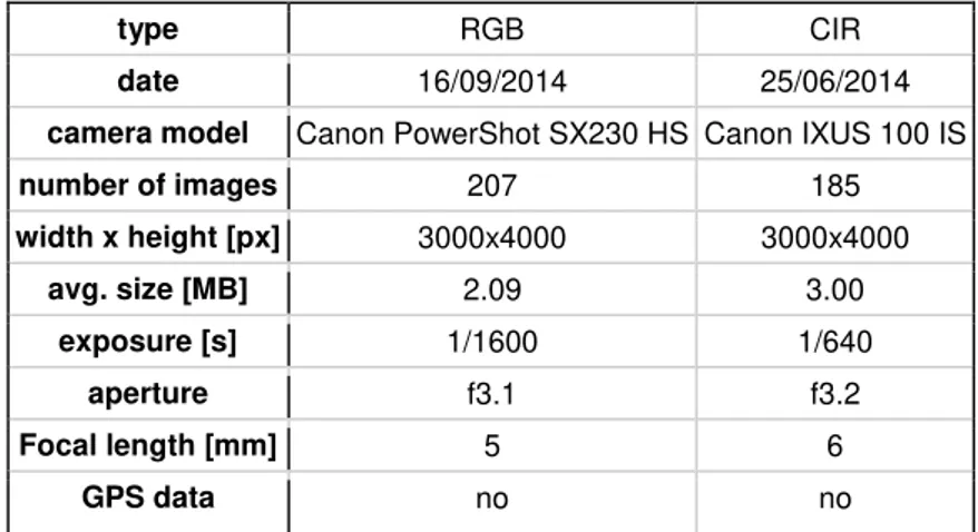
Imagery was obtained in different flight campaigns, using cameras able to capture RGB and NIR wavelengths. First campaign was performed by research team on 16/09/2014 using Canon PowerShot SX230 HS. 207 RGB images were collected. Second campaign was conducted by the team on 25/06/2014 using modified Canon IXUS 100 IS. The so called „hot filter‟ filtering NIR in most commercially available cameras was removed. Due to this modification, camera sensor was able to capture NIR wavelengths. The advantage of this modification consists in higher flexibility of image acquisition regimes, as user can decide in which mode the images will be taken by placing respective external filters in front of the camera (LEHMANN et al., 2015). As cameras usually do not have specified channel for NIR wavelengths, these have to be stored in one of the three channels of the sensor. Thus the camera used in this work had attached Cyan color filter to exclude the visible red light and allow the NIR radiation of up to 830nm to be recorded in Red band of the sensor. Camera captured visible and NIR wavelengths simultaneously. The Red light wavelengths were not captured anymore, thus the resulting false color composites were composed by captured NIR, Green and Blue bands. Similar approach was used by Hunt et al. (2010). More details about this technology can be found in (LEHMANN et al., 2015). 185 CIR images were collected using this camera during the second flight campaign. Details of the imagery can be found in Tab. 1.
type RGB CIR
date 16/09/2014 25/06/2014 camera model Canon PowerShot SX230 HS Canon IXUS 100 IS
number of images 207 185
width x height [px] 3000x4000 3000x4000
avg. size [MB] 2.09 3.00
exposure [s] 1/1600 1/640
aperture f3.1 f3.2
Focal length [mm] 5 6
GPS data no no
25
3.2.3 GPS data
There were two types of GPS data collected by the team. Firstly, 15 Ground Control Points (GCPs) were collected using GPS receiver with vertical accuracy of 8.5 cm and horizontal accuracy of 5.7 cm. Next, Differential GPS measurements of Acacia trees in the area were collected. 438 records were captured in the whole area. The overview of data and segments location can be seen on Img. 7.
26
4
Implementation
Workflow leading to the extraction of the products such as orthoimagery and digital surface elevation model suitable for further processing involves two main stages. First stage consists of a fieldwork - photo acquisition and GPS measurements (GCPs and DGPS acacia truthing collection). Second stage is then the processing of raw images and GPS data. DGPS measurements have to be corrected. Images of low quality have to be sorted in order to avoid false matches. Image matching is then performed using different software - PhotoScan and VisualSfM. Both workflows fundamentally present similar approach, however due to software capabilities there are some differences in the order of the performed steps - namely, georeferencing part in case of PhotoScan can be done immediately after sparse cloud reconstruction.
The processing steps were done using high-performance PC with NVIDIA Tesla C1060 GPU (4GB GPU memory, 240 cores).
4.1
Data preparation
4.1.1 Differential GPS correction
Acacia ground truthing DGPS records had to be corrected in order to reach higher accuracy. Corrected data were consequently used as GCPs as well as for visual detection of the Acacias on the imagery. The DGPS correction was performed using GTR Processor software package. Images were corrected using Brazilian Network for Continuous Monitoring of the GNSS Systems in real time (RBMC), real-time positioning service for DGPS measurements (IBGE, 2015). Finally, 438 records were corrected utilizing Teixeira de Freitas (BATF) reference station and exported into WGS84 / UTM 24 S coordinate system.
4.1.2 Image selection
27
UAS GPS module. The blurred images, high angle oblique images and images not covering the area of interest were filtered resulting in dataset of 195 RGB images and 143 CIR images.
4.2
Image processing using Agisoft PhotoScan
28
Img.
8.: Workflow diagram of data pre-processing using PhotoScan.
4.2.1 Feature detection and matching
After loading the images into PhotoScan, the first step is to align the images. This procedure is based on the feature detection and matching allowing to estimate positions of the cameras. Thus, this step is important, as point cloud densification can perform good only if sufficient amount of the cameras have known IO and EO parameters. The three involved processes are implemented in PhotoScan as a single step. PhotoScan provides three parameters influencing the final result of the image stitching. Meaning of the parameters is presented below:
Accuracy - controls the accuracy of camera position estimates. Lower accuracy results in lower precision and shorter computation time (AGISOFT LLC., 2014).
29
their position. Generic option chooses overlapping images by matching them firstly using low accuracy (AGISOFT LLC., 2014).
Point limit - upper limit of the feature points detectable in the image (AGISOFT LLC., 2014).
In order to estimate a parameter setup with the best performance, feature detection, matching and bundle adjustment were performed using various combinations of the parameters. As mentioned before, number of images with successfully estimated IO and EO parameters is important in order to perform further steps, thus this is the main criterion for the assessment of the process quality. In terminology of PhotoScan, images with known IO and EO estimates are called "aligned".
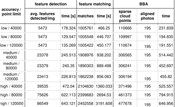
Images of both datasets were matched using Generic method. In both datasets matching was tested using different values of Accuracy parameter (low/medium/high) and different values of Point limit parameter (40000/80000/120000). Consequently the best matching results were taken for further processing. The results of stitching using different parameters can be seen in Tab. 2. and Tab. 3.
accuracy / point limit
feature detection feature matching BBA
avg. features
detected/img time [s] matches time [s]
sparse cloud points
aligned
photos time
low / 40000 5473 178.324 1005761 466.25 110666 195 231.839
low / 80000 5473 129.547 1005548 446.707 109997 195 194.835
low / 120000 5473 135.269 1005422 450.177 110674 195 191.551 medium /
40000 23378 245.513 1908976 938.202 306565 195 514.442 medium /
80000 23379 240.35 1890303 889.498 306241 195 452.697 medium /
120000 23413 226.813 1862238 856.063 306194 195 455.82 high / 40000 39535 472.04 2104630 1360.033 371496 195 525.557
high / 80000 75626 622.113 2399683 2694.53 461373 195 794.915
high / 120000 86549 643.121 2452558 3191.608 477678 195 646.956
30
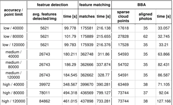
accuracy / point limit
featrue detection feature matching BBA
avg. features
detected/img time [s] matches time [s]
sparse cloud points
aligned
photos time [s]
low / 40000 5621 99.778 175581 216.138 17618 35 33.057
low / 80000 5621 101.79 175889 215.655 27828 62 32.745
low / 120000 5621 99.783 175939 216.376 17528 35 33.21 medium /
40000 26743 180.211 362748 311.86 54593 35 63.866 medium /
80000 26743 186.29 362666 337.874 54702 35 82.431 medium /
120000 26743 184.545 362662 328.77 54591 35 86.587 high / 40000 39972 348.567 399670 390.281 63469 38 71.105
high / 80000 78011 494.318 436569 799.127 73744 37 92.04
high / 120000 84862 461.015 437898 733.281 73744 38 127.166
Tab. 3.: Results of CIR imagery stitching using different variations of parameters using PhotoScan.
The decision of the final parameters chosen for the stitching was based on Tab. 2., Tab. 3. and visual assessment of the camera positions estimation quality. For the RGB dataset the parameters setup of Accuracy: high; Pair selection: Generic; Point limit: 80000 was chosen. Option using Point limit: 120000 parameter value returns similar performance, however processing time is higher. In case of CIR dataset, the setup of Accuracy: low; Pair selection: Generic; Point limit: 80000 was chosen as a suitable configuration due to nearly doubled amount of aligned imagery compared to other cases.
31
4.2.2 Georeferencing and camera optimization
Georeferencing was done using provided DGPS measurements. In order to perform comparison of the results later in this work, subset of DGPS measurements was used, as the different workflows and datasets do not provide exactly the same extend of area covered. Thus a set of Acacia measurements were used in the both datasets. However, it was not possible to use exactly the same points in both cases. Both datasets were georeferenced in WGS84 / UTM 24 S projection. In case of the RGB dataset, 14 GCPs were used. While working with CIR dataset 10 GCPs were placed successfully. Consequently, based on provided GCPs the IO, EO parameters and point coordinate estimates were optimized.
4.2.3 Point cloud densification
Next step in the workflow was the point cloud densification. This step creates dense point cloud based on the sparse cloud reconstructed in previous step. Agisoft offers two parameters to control this process: Quality and Depth Filtering Mode. While Quality parameter provides control over the quality of resulting cloud (higher quality brings higher computation time), Depth Filtering Mode controls outliers filtering (AGISOFT LLC., 2014). In case of the both datasets the parameters were set according to the software recommendations and time processing constraints as follows: Quality: Medium, Depth Filtering Mode: Aggressive. The occurring outliers were removed by manual editing.
4.2.4 Mesh reconstruction
32
With respect to the software recommendations the parameters for both datasets were set to: Interpolation: enabled, Source data: dense point cloud, Polygon count: high, Surface type: height field.
After the mesh reconstruction the DSM and orthophoto export is enabled. For the RGB dataset, both of these were exported, while for the CIR dataset only latter of the two, as during the previous processing the RGB dataset showed higher number of aligned imagery caused by sufficient image overlap. DSM and orthophotos were exported as .TIFF format files with spatial resolution 5 cm/pix. Img. 9. and Img. 10. are showing the sparse point cloud, dense point cloud and mesh of the both datasets.
Img. 9.: Sparse point cloud (a), dense point cloud (b) and mesh (c) created based on RGB imagery.
33
4.3
Image processing using VisualSfM
VisualSfM software presents GUI approach for SfM algorithms execution. In contrast with the previous solution algorithms used in the software are publicly known. General workflow involves image loading followed by the feature detection, matching and bundle adjustment resulting in a sparse point cloud. Once the cloud is generated additional cloud densification can be performed in case the CMVS/PMVS2 software library was previously installed. VisualSfM however provides only limited option for georeferencing, thus in this workflow additional open-source software combination was used for this task. Next, VisualSfM does not provide an option to generate and edit mesh nor export DSM and orthophoto directly. Due to this reasons, the workflow includes usage of CloudCompare (CLOUDCOMPARE, 2015) software in combination with GRASS GIS in order to georeference the point cloud. After the cloud is transformed, interpolation can be performed either using open-source QGIS or commercial ArcGIS software. Orthoimagery generation was achieved using CloudCompare which undistorts input imagery based on camera parameters estimated by VisualSfM. Images processed in this manner can be stitched using free tool MicrosoftICE or similar. Additional georeferencing of the created orthoimagery has to be performed. VisualSfM allows to adjust some of the processing parameters directly from GUI, however full parameter list is stored in nv.ini file. Both datasets were processed in the same manner. DSM export was performed only for RGB data due to the same reasons as in the previous workflow. VisualSfM 0.5.26 (64bit) version was used in this workflow. Schema of proposed workflow can be seen on Img. 11.
34
Img. 11.: Schema of VisualSfM-based workflow.
4.3.1 Feature detection
35 4.3.1.1 DIM parameter
DIM parameter, in VisualSfM nv.ini file internally called maximum_working_dimension adjusts the dimensions of imagery in case a higher from its two dimensions exceeds given threshold (WU, 2015d). This adjustment is performed due to processing time savings. The parameter can be adjusted manually in case of a higher precision demands and suitable hardware equipment. Dimensioning principle in SiftGPU works as shown below (WU, 2015d):
d = max(width, height);
sz = 2*d
sz' = max{sz / 2i | sz / 2i <= DIM, int i >= 0}
Thus, images are down-sampled or up-sampled prior to the processing dependent on their size. Default value of the DIM parameter is set to 3200. In such a case, imagery with dimension e. g. 1600 x 800px (d = 1600) would be up-sampled to 3200, while imagery of d = 4000 would be down-up-sampled to 2000. As the data used in this work are of the dimension 3000x4000px, the DIM parameter was set to a value 4096. Another possibility is to down-sample the data to 3200px however this would lead to a loss of information (WU, 2015d).
4.3.1.2 TC parameter
TC parameter represents approximate limit of detectable features per image. It comes with 4 options where (WU, 2015a):
-TC, -TC1 option keeps the amount of detected features high above the given limit set by numeric value.
-TC2 is similar to -TC and -TC1, however processing should be performed faster.
36
Setting the value to -1 allows detection without any limitation. Default value of the parameter is set to -TC2 7680, meaning that the amount of detected features should exceed the given value.
The feature detection was performed using CUDA. VisualSfM stores detected features in binary format .SIFT, thus the features can be used or extracted by external program. In this work, TC2 parameter values of the feature detection were set to 4000, 8000, 12000 and -1 (no limit).
4.3.2 Feature matching
Feature matching was performed by the SiftGPU as well. User can choose between CPU or GPU (CUDA or GLSL) implementations. Instead of the full matching, Visual SfM provides option to execute the preemptive version of the matching approach. Additionally software allows to compute matches for a given pairs and to visualize matching matrix expressing intensity of matching relation between all images.
4.3.3 MaxSIFT parameter
Main parameter influencing matching result is the MaxSIFT, in nv.ini referenced as param_gpu_match_fmax. This parameter determines the number of features per image used in matching (WU, 2015d). As the preemptive matching is in use, the features are sorted by scale in a decreasing order. Rising the parameter value thus allows to match also features in a smaller scales. Default value of this parameter is set to 8192, however according to the authors recommendation value 4000 would be sufficient in most of the cases (WU, 2015d).
37
4.3.4 Sparse cloud reconstruction
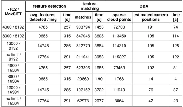
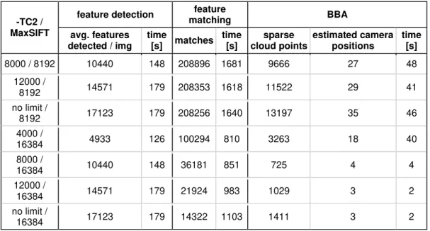
Consequent step after the matching is the bundle adjustment resulting in camera positions estimation and sparse cloud reconstruction. In this step VisualSfM allows to adjust a set of parameters related to the number of iterations in bundle adjustment, frequency of global or partial adjustment execution, MSE threshold or number of imagery used in every partial bundle iteration (WU, 2015d). Sparse cloud reconstruction for every parameter combination described above was performed without adjustment of the BBA parameter. Results of the feature detection, matching and sparse cloud reconstruction are shown in Tab. 4. and Tab. 5.
-TC2 / MaxSIFT
feature detection matching feature BBA
avg. features detected / img
time
[s] matches time [s] sparse cloud points estimated camera positions time [s] 4000 / 8192 4765 257 903794 1453 72700 191 74
8000 / 8192 9685 315 847046 3608 113450 195 114 12000 /
8192 14745 285 812779 3884 114310 195 125 no limit /
8192 17764 291 211041 3958 115327 195 122 4000 /
16384 4765 257 523396 1685 73463 192 81 8000 /
16384 9685 315 20869 190 1768 14 4 12000 /
16384 14745 285 102152 3722 11949 76 37 no limit /
16384 17764 291 62973 2077 3064 42 23
Tab. 4.: Results of RGB imagery stitching using different variations of parameters in VisualSfM.
-TC2 / MaxSIFT
feature detection feature
matching BBA
avg. features detected / img
time
[s] matches time [s] sparse cloud points estimated camera positions time [s] 4000 / 8192 4933 126 100294 802 8045 27 41
8000 / 8192 10440 148 208896 1681 9666 27 48
38
-TC2 / MaxSIFT
feature detection feature
matching BBA
avg. features detected / img
time
[s] matches time [s] sparse cloud points estimated camera positions time [s] 8000 / 8192 10440 148 208896 1681 9666 27 48
12000 /
8192 14571 179 208353 1618 11522 29 41 no limit /
8192 17123 179 208256 1640 13197 35 46 4000 /
16384 4933 126 100294 810 3263 18 40 8000 /
16384 10440 148 36181 851 725 4 4 12000 /
16384 14571 179 21924 983 1029 3 2 no limit /
16384 17123 179 14322 1103 1411 3 2
Tab. 5. - continue: Results of CIR imagery stitching using different variations of parameters in VisualSfM.
Based on the Tab. 4. and Tab. 5. results with the highest number of camera parameter estimations were taken for further processing. In case of the both datasets this was achieved by using -TC2 / MaxSIFT parameters setup values no limit / 8192.
Prior to the cloud densification, tools for manual alignment of the cameras without estimated parameters were used. VisualSfM provides Spanning Forest tool allowing to visualize the matching relationships between imagery. According to the settings, the software can search either for only one model or for several models during the sparse cloud reconstruction. If only one model is searched the result with the highest amount of solved cameras is provided. In case of the multiple search all models are returned, however disconnected. Spanning tree tool allows to detect visually the images between models with a weak links. After the pairs of images with the weak linkage are detected, additional feature detection and matching for the given pairs can be executed. In this manner CIR model was manually edited resulting in a merge of two models providing totally 46 solved cameras.
39
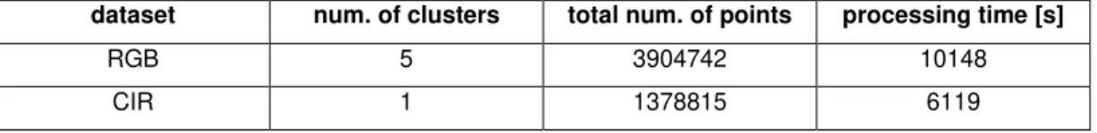
4.3.5 Cloud densification
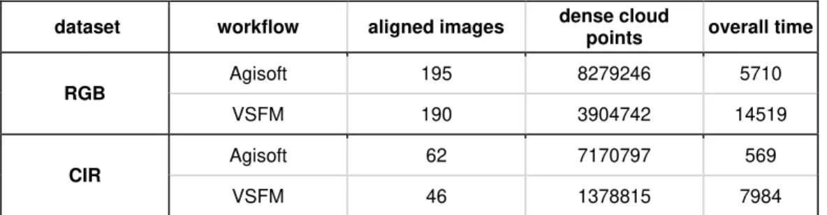
Cloud densification was performed using the CMVS/PMVS2 package. In VisualSfM both softwares are used in one step, however the process can be divided into two parts. First CMVS decides the amount of clusters in which the input data are divided. Those are then passed to the PMVS2 for cloud densification. Output is then stored in .PLY files, which amount depends on the amount of the clusters. Densification of RGB dataset results can be seen in Tab. 6.
dataset num. of clusters total num. of points processing time [s]
RGB 5 3904742 10148
CIR 1 1378815 6119
Tab. 6.: Details of point cloud densification using CMVS/PMVS2.
4.3.6 Point cloud georeferencing and DSM export
As VisualSfM does not support direct export of the DSM nor orthoimagery, both products can be obtained using third party software. DSM export was performed only for point cloud derived from the RGB dataset, as more cameras were solved and thus the point cloud provides better area coverage.
40
Transformed point cloud was imported into ArcGIS software, where ASCII 3D to Feature Class tool was used to export the point cloud into GIS format (.SHP file). The same can be achieved using Add Delimited Text Layer tool in QGIS. After the import, Inverse Distance Weighted (IDW) interpolation was used for the DSM interpolation.
4.3.7 Orthophoto export and georeferencing
Due to the lack of orthophoto export feature in VisualSfM, additional software pipeline had to be utilized. The CloudCompare software allows to import the output file of VisualSfM containing camera parameters estimation (.OUT format). As a part of the import, CloudCompare provides option to undistort imagery based on the parameters contained in the file. Imagery of the both datasets was undistorted in this manner. Consequently, image stitching software Microsoft ICE was used in order to stitch the images together.
41
5
Acacia tree classification
In this chapter the practical usage of extracted DSM and orthophoto will be demonstrated on the Acacia detection. Products will be enhanced and different classification workflows will be proposed using the RGB and CIR datasets respectively. Classification based on RGB dataset will use the DSM elevation data, while classification using CIR data will use BNDVI. Both classifications will be tested with and without inclusion of the IHS bands in order to examine its contribution to the classification accuracy. Two areas will be chosen for classification model development and testing (Segment 1 and Segment 2 respectively). Workflows will use data derived from PhotoScan-based workflow. Classification rulesets were developed using Trimble eCognition Developer 8 software.
5.1
Data enhancements
In order to get advantage of the information provided by NIR band in the CIR dataset, NDVI based on Blue band (referenced as BNDVI) was calculated following the formula (1). Blue band was chosen due to the lack of a Red band in the imagery. Another enhancement was done by transforming both datasets to the IHS color space. Software used for performing these steps was PCI Geomatica (Raster Calculator and RGB to IHS tools).
Next, absolute height data extracted from the RGB dataset had to be transformed into relative information. Absolute information provided by DSM would produce false assumptions about vegetation height, as the terrain slope would influence final vegetation height. Transformation can be done by subtracting absolute heights of terrain (DTM) from absolute heights of the surface model (DSM) resulting in the Surface band. The DTM was generated using PCI Geomatica‟s DSM2DTM algorithm. Raster-to-raster calculation was performed
using Raster Calculator tool in ArcGIS.
42
5.2
Classification schema and spectral behavior
Classification schema was defined based on a main land cover types and their illumination properties observable on the imagery. The classification followed hierarchical structure thus the classes for the both classifications were organized in hierarchies. Each hierarchy consists of two levels: Classification Level 1 and Classification Level 2. Class definitions differ for each dataset.
Classification Level 1 of CIR dataset is formed by two main land cover types present on the imagery - Non-vegetation and Vegetation superclasses. The former was not examined more in detail, however classes of Soil and Shadows can be implicitly included in this superclass. Vegetation superclass consists of following classes: Acacia bright, Acacia dark, Shrub bright, Shrub dark, High grass bright, High grass dark, Dry grass/soil mix medium, Dry grass/soil mix strong.
Classification schema for RGB dataset differ in structure as the classification is based on surface elevation (Surface band). Classification Level 1 is formed by Low vegetation and High vegetation superclasses. While the former is not a subject of the interest, latter one is subdivided into Acacia bright, Acacia dark, Shrub bright and Shrub dark children classes. Finally in both workflows classes were aggregated into Acacia and Non-Acacia classes. The classification and aggregation schema can be seen in Tab. 11. and Tab. 12., Appendix B. In order to get insight into spectral behavior of different classes, spectra plots for both datasets were created (Img. 13 and Img. 14.).