ISSN 0101-8205 / ISSN 1807-0302 (Online) www.scielo.br/cam
An overview of flexibility and generalized
uncertainty in optimization
∗WELDON A. LODWICK
University of Colorado Denver, Department of Mathematical and Statistical Sciences Campus Box 170, P.O. Box 173364, Denver, CO 80217-3364, U.S.A.
E-mail: [email protected]
Abstract. Two new powerful mathematical languages, fuzzy set theory and possibility theory,
have led to two optimization types that explicitly incorporate data whose values are not real-valued nor probabilistic: 1) flexible optimization and 2) optimization under generalized uncertainty. Our aim is to make clear what these two types are, make distinctions, and show how they can be applied. Flexible optimization arises when it is necessary to relax the meaning of the mathematical relation of belonging to a set (a constraint set in the context of optimization). The mathematical language of relaxed set belonging is fuzzy set theory. Optimization under generalized uncertainty arises when it is necessary to represent parameters of a model whose values are only known partially or incompletely. A natural mathematical language for the representation of partial or incomplete information about the value of a parameter is possibility theory. Flexible optimization, as delin-eated here, includes much of what has been called fuzzy optimization whereas optimization under generalized uncertainty includes what has been called possibilistic optimization. We explore why flexible optimization and optimization under generalized uncertainty are distinct and important types of optimization problems. Possibility theory in the context of optimization leads to two dis-tinct types of optimization under generalized uncertainty, single distribution and dual distribution optimization. Dual (possibility/necessity pairs) distribution optimization is new.
Mathematical subject classification: 90C70, 65G40.
Key words: fuzzy optimization, possibility optimization, interval analysis, generalized
uncertainty.
#CAM-702/12. Received: 22/IX/12. Accepted: 28/IX/12.
1 Introduction
between classical deterministic linear programming and what is actually done in practice.
Secondly, many data of parameters to an optimization problem are described by incomplete, poorly specified, imprecise data. We will limit ourselves to in-complete information in the data that generate pairs of functions that bound the imprecision arising from the partial information. When this is the case in the con-text of optimization, we will argue that optimization that takes into consideration the entire set of functions delineated by the pair of bounding possibility func-tions is a useful way to optimize. Generalized uncertainty that lead to bounding possibility pairs are fuzzy intervals (defined below), interval-valued probability [35], belief/plausibility measures over nested focal elements [2, 17, 29], clouds [26], p-boxes [7], and random sets [27] over nested focal elements.
Thus, our contribution in this overview is to present flexible optimization and optimization under generalized uncertainty in a clear way, highlighting their im-portance, illustrating their applicability, distinguishing flexible and possibilistic optimization, and introducing a new approach to optimization under generalized uncertainty, the dual distribution optimization.
We conclude our introduction with a short description of fuzzy set theory, pos-sibility theory, generalized uncertainty, and the statement of our optimization problem. The second section looks at the entities most relevant in flexible and generalized uncertainty optimization. The third section addresses the optimiza-tion types themselves and we make concluding remarks in the fourth secoptimiza-tion.
1.1 Fuzzy sets
Fuzzy sets encode transitional or gradual set belonging.
Definition 1.Fuzzy set: [36] A fuzzy set is a set whose elements possess a degree of belonging to the set, where the degree is given by a value in the interval [0,1]. A fuzzy set is uniquely defined by a membership function μA : X → [0,1], A ⊆ X,whereμA(x)denotes the degree to which the element x belongs to the fuzzy set A. We adopt the convention that the membership function of the empty set is zero.
or not. Thus, a set is a fuzzy set if belonging is transitional rather than Boolean. Practically speaking, since we are interested in quantitative optimization, we are interested in fuzzy sets over the real numbers and we will assume that the universal set from which we define a fuzzy set is the set of real numbers. A fuzzy set, say A, is uniquely defined by a continuous concave function μA whose
support is compact and whose range is a subset of[0,1]. That is, given a support of[a,b], μAis a continuous concave function on[a,b]where
y =μA(x)=
(
y∈ [0,1] for a≤ x ≤b y=0 otherwise .
There are generalizations to the assumptions made on the membership function such as upper semi-continuity rather than continuity, but we will not pursue these for this exposition. What is important to note is that in the language of fuzzy sets, μA(x)=1 means thatx belongs to the setAin the classical sense of belonging
(belongs for sure) andμA(z) =0 means thatz does not belong to set Ain the
classical sense of not belonging (does not belong for sure). All values between 0 and 1 denote the transition from belonging to not belonging. The mathematical language of flexibility and the associated algebra and analysis of this language is fuzzy set theory. The flexibility as developed here is modeled in its native setting as transitional set membership (belonging). To be sure, one translates the problem into a approximate real-valued problem. This type of translation is also done in stochastic optimization problems.
1.2 Generalized uncertainty
membership functionμA(x)and so is distinct from uncertainty which models
partial or incomplete information.
Generalized uncertainty is uncertainty that is not only tied to information deficiency but is any uncertainty that is non-deterministic and non-unique prob-abilistic. Generalized uncertainty has an associated set of distributions (bounded above and below) that contains the unknown distribution. It is uncertain because it is not known which of the distributions in the set is the appropriate one(s). It is generalized uncertainty since it includes more than deterministic uncertainty (error) and probabilistic uncertainty. We will pay special attention to possibility as one type of generalized uncertainty which is particularly useful since it is rela-tively easy to use in optimization, has a rich semantic with an algebraic structure that is able to model problems in which the data arises from partial/incomplete information.
There are four generalized uncertainty types that can be transformed into possibility/necessity pairs: 1) intervals, 2) interval-valued probability distribu-tion (IVPD) pairs [35], 3) clouds [26] Figures 3, and 4) fuzzy interval (see Fig. 2). More general forms of generalized uncertainty exist, for example be-lief/plausibility pairs [29] and random sets [27] whose focal elements are nested, but our focus here are these four types (intervals, IVPDs, clouds, fuzzy intervals) because there exist methods to directly translate these into possibility/necessity pairs. Possibility, generally speaking, is a term that we use as the model of lack of information about the value of an entity. Its definition, is as follows.
Definition 2. Apossibility measureis a set-valued function over theσ-field of a universal set X ,
P : A⊂σ (X)→ [0,1]such that
Pos(∅) = 0, Pos(X)=1, (1)
Pos(A∪B) = max{Pos(A),Pos(B)}. (2)
There are some continuity assumptions that sometimes are made such as:
Given A1⊆ A2⊆. . .⊆ An⊆. . .such that lim
n→∞An = A, then
lim
Remark 1. Given (1) and (2), we can show: 1) monotonicity, that is,A⊆ B⇒
P(A) ≤ P(B), 2) an underlying nested set of subsets ofσ (X)exists such that beginning with the nested set, we can define the possibility for all sets of our σ-field. Moreover, given a possibility on a nested set of sets of theσ-field (with the boundary conditions), we can define a possibility on all of theσ-field such that the possibility of a union of two sets is equal to the maximum of the two possibilities (see [17, 33]). Therefore, given (1) and (2) a generating nested set of subsets can be constructed so that on this nest (1) and (2) hold. On the other hand, given a nested set of subsets on which (1) and (2) hold, we can define a possibility measure on the entireσ-field such that (1) and (2) holds on theσ -field. The significance of this fact in terms of optimization is that when a random set or a belief/plausibility measure has nested focal elements, we can define a bounding pair of possibility measures that encloses the uncertainty as defined by the random set (or belief/plausibility).
Given a possibility measure (function on sets), apossibility distribution is a function (on elements of the universal set)
p(x):X → [0,1],p(x)= P({x}).
Since we will be dealing, in optimization, with existent objects, there is at least onex ∈ X such p(x) =1. Given apossibility measure, its dual N ec, called a
necessity measure, is defined by
N ec(A)=1−Pos(AC), (3)
for any measurable set A ⊂ X, where AC is the complement of A. Given (1), (2) and (3), it is easily shown that,
N ec(∅) = 0,N ec(X)=1,
N ec(A∩B) = min{N ec(A),N ec(B)}.
The dual of a possibility distribution, called anecessity distribution, is the func-tion
n(x): X → [0,1],n(x)=N ec({x}).
If we know the possibility of a set A, the possibility of the complement of A,
Pos(AC), is not derived as Pos(AC) = 1 − Pos(A) in contradistinction to probability, its dual, necessity is required [3]. That is,N ec(A)=1−Pos(AC),
1.3 Optimization
A real-valued (deterministic) optimization problem has the general form:
z = min f(c,x), (4)
subject to gi(a,x) ≤ b i =1, . . . ,M1, (5)
hj(d,x) = e j =1, . . . ,M2. (6) The constraint set is denoted by
= {x|gi(x,a)≤bi, i =1, . . . ,M1,hj(x,d)=ej, j =1, . . . ,M2}.
It is assumed that 6= ∅. The values of a,b,c,d and e are data, parame-ters. Thus, to highlight the main thesis of this study, our general model can be reformulated as
z = min f(x,c)
x ∈ (a,b,d,e),
where we denote the constraint set as a function of the input parameters for emphasis. From our point of view, when the ∈of “element of ” is relaxed, then we have flexible optimization. The constraint setiscrisp,real-valued, but belonging tois soft, transitional, or gradual. From the point of view of generalized uncertainty, data,a,b,d,e, that arises from incomplete, imprecise information generate a constraint setthat is defined by aset of distributions. Likewise, if data elementc is a generalized uncertainty type, the objective is a sets of enclosed functions.
2 Fundamental entities of generalized uncertainty analysis
We outline the relationship between fuzzy intervals and possibility distributions next.
2.1 Intervals
An interval is a compact connected set of real numbers X = [x,x] = {x|x ≤
distributions and indeed level sets of fuzzy numbers are intervals. In particular, one way to compute with generalized uncertainties is via intervals arising from level sets and hence we discuss intervals in a little bit of detail next.
An interval may be considered as a type of fuzzy interval (see Fig. 1). An interval possesses a triple nature, that of an interval number [x] ≡ {x,x} con-sisting of two elements (and ordered pair of numbers(x,x),x ≤x), that of aset
[x] = {x|x ≤x ≤x}, or that of a single-valued linear function with non-negative slope over the compact real set[0,1],
f(λX)=wXλX+x, 0≤λX ≤1, wX =x −x ≥0. (7)
This third view we call aconstrained interval(see [18]) because the variableλX
is constrained to be in[0,1]. This point of view means that intervals belong to a space of linear single-valued function over compact domains with non-negative slopes which is distinct from the space of interval numbers which is the upper left half-plane inR2determined byy ≥x. We favor this third view of intervals since it yields a richer algebraic structure. Intervals may model non-specificity or information deficiency. At the same time, intervals may also represent a fuzzy set, a fuzzy interval (number), with a membership function
μ[a,b]= (
1 x ∈ [a,b]
0 otherwise . (8)
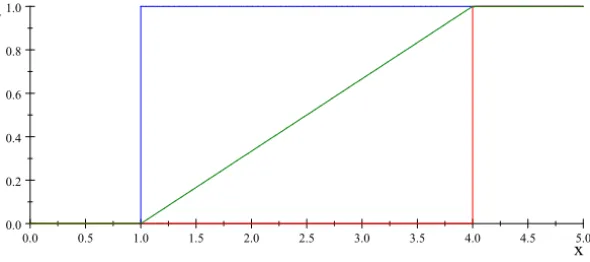
For example, if we have an interval [1,4], then it can represent a fuzzy set μ[1,4] in the sense of (8) (see Fig. 1). However, the interval [1,4] as a piece
of partial or incomplete information of an unknown value, defines upper and lower possibilities that bound all (cumulative) distributions whose supports are in[1,4]. That is, in the context of sets of probabilities, if all that is known is that the support of the probability lies in the interval[1,4], the possibility
p(x)= (
1 if x ∈ [1,∞)
0 if x ∈(−∞,1) (9)
and necessity
n(x)= (
1 if x ∈ [4,∞)
pair boundall cumulative probability distributions that have support in[1,4]. Note that the middle possibility distribution
u(x)=
1 3x −
1
3 if x ∈ [1,4] 1 if x ∈ [4,∞) 0 otherwise
(11)
is the cumulative of the uniform distribution whose support is[1,4]and corre-sponds to choosing a “midpoint”. The cumulative representing the entire prob-ability being 1 (the real number 1), is the possibility (9). The cumulative repre-senting the entire probability being 4 (the real number 4), is the necessity (10). We prove that this is true in the general case of an arbitrary fuzzy interval in the next section.
0.0 0.5 1.0 1.5 2.0 2.5 3.0 3.5 4.0 4.5 5.0
0.0 0.2 0.4 0.6 0.8 1.0
x y
Figure 1 – An interval as a possibility/necessity pair.
2.2 Fuzzy intervals
The entities of analysis that are used in flexible and generalized uncertainty optimization are calledfuzzy numbersand their generalizations are calledfuzzy intervalswhich we formally define next.
0 1 2 3 4 5 6 7 0.0
0.2 0.4 0.6 0.8 1.0
1
y
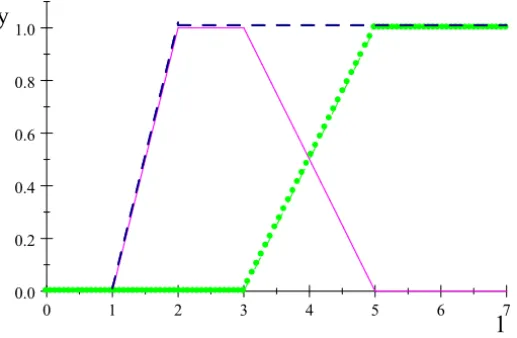
Figure 2 – Fuzzy interval – possibility, necessity.
There are various views and applications of fuzzy intervals. A fuzzy interval can be used to enclose a set of probability distributions where the bounds are constructed from the fuzzy interval (dashed black line being the possibility and dotted gray line being the necessity in Fig. 2). To prove this, let μ(x)be the membership function of a fuzzy interval and Pr(A)be probability measures for which
sup
a∈A
μ(a)≥Pr(A) (12)
whereA=(−∞,x]forx ∈R. Define
Pos(A)=sup
a∈A
μ(a). (13)
Pos(A)so defined, is a possibility measure since
Pos(∅) = sup
a∈∅
μ(a)=0
Pos(X) = sup
a∈X
μ(a)=1, and
Pos(A∪B) = sup
x∈A∪B
μ(x)
= sup
x∈A
μ(x)or sup
x∈B
μ(x)
= max{sup
x∈A
μ(x), sup
x∈B
μ(x)}
Thus,Pos(A)defined by (13) satisfies (1) and (2) and so it is a possibility. Given this definition of possibility (13), the following holds.
Pos(A) = sup
a∈A
μ(a)≥Pr(A)for all measurableA.
N ec(A) = 1−Pos(AC)or
Pos(AC) = 1−N ec(A). Now,
Pos(AC) ≥ Pr(AC)=1−Pr(A)or
Pr(A) ≥ 1−Pos(AC)= N ec(A). Thus,
N ec(A) ≤ Pr(A)≤ Pos(A). (14)
That is, when we define a possibility by (13), we generate a possibility/necessity dual pair of bounding measures for all probabilities that satisfy (12). Therefore, a fuzzy interval can be viewed as encoding a family of probabilities, the set of probability measures Pr(A) defined by (12). Thus, a fuzzy interval, as a piece of incomplete information, encodes a family of probability bounded by a possibility/necessity pair (14).
2.3 Possibility intervals
The mathematical structure of possibility theory was first developed by [37] and more extensively articulated in [3, 4]. There are several ways to construct possibility and necessity distributions from generalized uncertainty types. We highlight four ways one can generate possibility/necessity pairs.
1. [22] Given a set of probability measures 4 = {pr obα(A),pr obα(A) ∈ L⊆R, α ∈ I,where I is an index set,La set of measurable subsets of R},
Pos1(A) = sup
α∈I
pr obα(A),pr obα(A)∈4, (15) N ec2(A) = inf
α∈I pr obα(A),pr obα(A)∈4. (16)
(ap-box, [7]), we can construct necessity and possibility (not necessarily duals) distributions such that the probability measure is bounded by
Pr(A)∈ [N ec2(A),Pos1(A)], (17) for all measurable setsA.
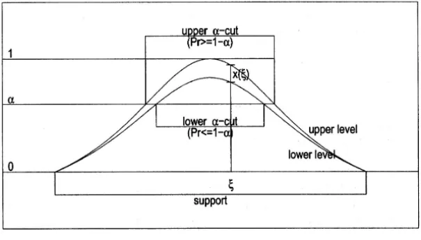
3. [26] Given a cloud (see Fig. 3), it can be translated into a possibility/ne-cessity pair (see [19]) where a cloud over a set M is a mapping x that associates with eachξ ∈ Ma (non-empty, closed and bounded interval)
x(ξ ), such that,
(0,1)⊆ [
ξ∈M
x(ξ )⊆ [0,1]. (18)
A real cloudy number is a cloud over the set Rof real numbers. χ[a,b] (χbeing the characteristic function) is the cloud equivalent to an interval [a,b]. That is, an interval provides only information about the support without additional probabilistic content. A cloudy vector is cloud overRn, where each component is a cloudy number. In many applications the level
x(ξ )may be interpreted as giving lower and upper bounds on thedegree of suitabilityofξ ∈ Mas a possible scenario for data modeled by the cloud
x. This degree of suitability can be given a probability interpretation by relating clouds to random variables, (19).We say that a random variablex
with values inMbelongs to a cloud xoverM, and writex ∈x, if Pr(x(x)≥α)≤1−α ≤Pr(x(x) > α) ∀α ∈ [0,1]. (19) This approach gives clouds an underlying interpretation as the class of random variablesx withx ∈x.
4. Given a fuzzy interval, one can generate a possibility/necessity pair using (13) and (3) such that (14) holds.
Figure 3 – Cloud.
3 Intervals, fuzzy set theory, and possibility theory in optimization
We next look at optimization according to the nature of the constraint set. Intervals can represent uncertainty in a parameter value (a,b,c,d,e of (4), (5) and (6)). This is the point of view of [8, 11, 21, 22]. However, [24] and [30] approach interval linear programs from a strictly interval perspective, where [8] uses both views. Historically, intervals have been used in global optimization [16]. In fact, many interval analysis researchers maintain that interval analysis in optimization is part of deterministic global optimization. Its aim is finding good, provable bounds on ranges of functions that contain the global optima.
Our point of view for this exposition is that intervals may be used in and of themselves to represent uncertainties when all that is known are the bounds on parameters in which case an interval can model transitional set belonging (8) or the lack of information or specificity (9), (10).
3.1 Fuzzy and possibility optimization and semantics
Next what is meant by decision-making in the presence of flexibility and gener-alized uncertainty is defined [20].
That is,
sup
x∈
hF˜1(x), . . . ,F˜n(x)
, (20)
whereh : [0,1]n → [0,1] is an aggregation operator [17] often taken to be theminoperator, andF˜i(x) ∈ [0,1] is the fuzzy membership ofx
in fuzzy set F˜i. The decision space is a set of real numbers, and the
optimal decision satisfies a mutual membership condition defined by the aggregation operator h. This is the method of Bellman and Zadeh [1], Tanaka, Okuda and Asai [31, 32], and Zimmermann [38], who were the first (in this order) to develop fuzzy mathematical programming. While the aggregation operatorh historically has been theminoperator, it can be, for example, any t-norm that is consistent with the context of the problem and/or decision methods [15].
2. Possibility decision making: Given the set of real-valued decisions, , and the set of possibility distributions representing the uncertain out-comes from selecting decisionxE=(x1, . . . ,xn)T denoted9x = { ˆFxi,i =
1, . . . ,n}, find the optimal decision that produces the best set of possible outcomes with respect to an orderingUof the outcomes. That is,
sup
9x∈9
U(9x), (21)
whereU(9x)represents an “evaluation function” (loosely, utility) of the
set of distributions of possible outcomes9 = {9x|x ∈}. The decision
space9is aset of possibility distributions9x :→[0,1] resulting from
taking decisionx ∈ . For example, if Fˆx = ˆ2x1+ ˆ3x2, where2 andˆ 3ˆ are the possibility numbers 2 and 3, then eachxE=(x1,x2)T generates the possibility distributionFˆx = ˆ2x1+ ˆ3x2.
Remark 2. For fuzzy sets F˜i,i = 1, …,n, givenx,[ ˜F1(x), . . . ,F˜n(x)]Tis a
real-valuedvector. Thus, we need a way to aggregate the components of the vectors into a single real-value. This is done by a t-norm, min for example. For possibility, givenx, 9x = { ˆFxi,i = 1, . . . ,n}is a set of distributions, so we
3.2 Fuzzy decision making using fuzzy optimization – flexible optimization
Fuzzy decision making using fuzzy optimization was first operationalized by Tanaka, Okuda, and Asai [31, 32], and then by Zimmermann [38]. This approach, based on Bellman and Zadeh [1], transforms systems of inequalities Ax ≤ b
and the objective function into aspirations. The results are what is commonly calledsoft constraints, where the number b to the right of the inequality is a target such that, if the constraint is less than or equal to b, the membership value is one (the constraint is satisfied with certainty), and, if the constraint is greater thanb+d, (for ana-priori given d ≥ 0), the membership is zero (the constraint is not satisfied with certainty). Here, the objective function is translated into a target, sayz= f(x,c)≥t∗, andt∗translated into an aspiration. In between, the membership function is interpolated so that it is consistent with the definition of a fuzzy interval membership function in the context of the problem. Linear interpolation was the original form [38]. This models a fuzzy meaning of inequality that is translated into a fuzzy membership function and is the source of our use of the designation of flexible programming for these classes of optimization problems. Theα-level represents the degree of feasibility of the constraints, consistent with the aspiration that the inequality be less thanbbut definitely not more than b+d. Thus, the objective, according to [38], is to simultaneously satisfy all constraints at the highest possible level of preference as measured by theα-levels of the membership functions. The approach of [38] is not always Pareto optimal. It must be iterated – fix the constraints at bounds and re-optimize.
Another related form of flexibility is allowing constraint violations to be mea-sured by a possibility (necessity) or probability distribution [9]. These methods fall within a goal satisfaction approach in optimization in which the highest degree of feasibility (the goal in this case) is sought.
A different method is that of aggregate goal attainment which maximizes an overall measure of aggregate goal satisfaction. The aggregate sum of goal attainment focuses on maximizing the cumulative satisfaction of the goals. The surprise function [23, 25] is one such measure for an aggregate set of (fuzzy) goals. If
where the right-hand side values of the soft constraint are fuzzy intervals, the transformation into a set of aggregate goal satisfaction problem using the surprise function as the measure for the cumulative goal satisfaction is attained as follows. A (soft) fuzzy inequality (22) is translated into a membership function,μi(x)of
the fuzzy set{(Ax)i ≤ ˜bi}. The associated surprise function is
si(x)=
1 μi(x)
−1 2
. (23)
These functions are added to obtain a total surprise
S(xE)=X
i
si((AxE)i)=
X
i
1 μi(x)
−1 2
. (24)
Note that (24) is an aggregation operator. A best compromise solution based on the surprise function is given by the nonlinear optimization problem
min z = S(Ex)=X
i
1 μi(x)
−1 2
, (25)
subject to x ∈ (possibly hard constraints). (26) The salient feature is that surprise uses a dynamic penalty for falling outside pre-ferred membership values of one. The advantage is that the individual penalties are differentiable convex functions which become infinite as the values approach the endpoints of the support. Moreover, the sum of convex functions is convex so that a local optimal of (25), (26) is a global optimum. Additionally, this approach is computationally tractable for very large problems [23] and is Pareto optimal.
3.3 Single possibility distribution decision making
One method of generalized uncertainty optimization [13] allows all constraint violations at an established cost or penalty and minimizes the expected average, a generalization of expected value [12, 13]. This approach considers all possible outcomes as a weighted expected average penalty. The expected average may be considered to be a type of evaluation function (utility). This particular evaluation function takes violations as penalties on all outcomes of the constraints. It optimizes over sets of possibility distributions that define the preferred levels of violation. The approach used in [13] is a possibility generalization of the
3.4 Dual possibility distribution decision making under uncertainty
Dual distribution optimization is an optimization in which both upper and lower bounds on expectation given the uncertainty are constructed. Given the upper and lower expectation, methods that yield minimum maximum regret have been developed by [33] and [34] to obtain a satisficing compromise solution.
3.5 Mixed fuzzy and possibility decision making: mixed possibility and probability optimization methods
An optimization problem containing a mixture of uncertainty together in one or more constraints we calledmixed optimization. Problems in which one type of uncertainty or flexibility occurs in a parameter of a constraints and another uncertainty or flexibility parameter occurs in another constraint (each constraint having a single type of uncertainty or flexibility) have been studied by [21]. There are other problems in which two or more types of uncertainty occur in two or more parameters of a single constraint. Thus, within a quantitative setting, there are two cases for the mixed problem.
1. A problem that contains flexible constraints and generalized uncertainty parameters, but each type is in one constraint and each constraint has only one type:
(a) The flexible constraints can be translated using the surprise method according to [25] or by using theα-levels according to [38]
(b) The generalized uncertainty can be translated, for example, into pos-sibility constraint penalties according to [13]. The resulting trans-lated system is then optimized such that if α-levels are used one obtains a Pareto optimal by fixing constraints at bounds and re-optimizing. With the surprise approach, this is unnecessary. 2. Two or more uncertainty parameters appear in the same constraint: One
4 Conclusion
The data which goes into a flexible optimization and generalized uncertainty optimization problem were delineated and specified. Each type of data not only is comprised of a membership or possibilistic function, but possesses a semantic which is the crucial key in determining the optimization type with its associated solution method. It is not the functional representation (membership function, possibility distribution) of the data entity that determines the optimization type, it is the semantic, since the functional representation of a member function is indistinguishable from a possibility distribution. Moreover, our exposition em-phasized and delineated the differences between fuzzy set theory and possibility as it impacts optimization problems that use these entities. We indicated how the semantics are important in distinguishing which of the various approaches must be used in obtaining a solution.
REFERENCES
[1] R.E. Bellman and L.A. Zadeh,Decision-making in a fuzzy environment. Manage-ment Science, Serial B,17(1970), 141–164.
[2] A.P. Dempster,Upper and lower probabilities induced by a multivalued mapping. Annals of Mathematical Statistics,38(1967), 325–339.
[3] D. Dubois and H. Prade,Possibility Theory.Plenum Press, New York (1988).
[4] D. Dubois and H. Prade (eds.),Fundamentals of Fuzzy Sets.Kluwer Academic Press (2000).
[5] D. Dubois and H. Prade, Formal representations of uncertainty. Chapter 3 in. D. Bouyssou, D. Dubois and H. Prade (eds.), Decision-Making Process, ISTE, London, UK & Wiley, Hoboken, N.J., USA (2009).
[6] G. Fandel, PPS-Systeme: Grundlangen, Methoden, Software, Markanalyse. Springer-Verlag, Heidelberg, Germany (1994).
[7] S. Ferson, V. Kreinovich, L.R. Ginzburg, K. Sentz and D.S. Myers,Constructing Probability Boxes and Dempster-Shafer Structures.Sandia National Laboratories, Technical Report SAND2002-4015, Albuquerque, New Mexico (2003).
[9] M. Inuiguchi, H. Ichihashi and Y. Kume, Relationships between modality con-strained programming problems and various fuzzy mathematical programming problems.Fuzzy Sets and Systems,49(1992), 243–259.
[10] M. Inuiguchi, H. Ichihashi and H. Tanaka, Fuzzy programming: A survey of recent developments, in: R. Slowinski and J. Teghem (eds.), Stochastic versus Fuzzy Approaches to Multiobjective Mathematical Programming under Uncer-tainty, Kluwer Academic Publishers, Dordrecht (1990), 45–68.
[11] M. Inuiguchi and M. Sakawa, An achievement rate approach to linear pro-gramming problems with interval objective functions.Journal of the Operational Research Society,48(1997), 25–33.
[12] K.D. Jamison,Modeling uncertainty using probability based possibility theory with applications to optimization.Ph.D. Thesis, UCD Department of Mathematics (1998).
[13] K.D. Jamison and W.A. Lodwick, Fuzzy linear programming using penalty method. Fuzzy Sets and Systems,119(2001), 97–110.
[14] K.D. Jamison and W.A. Lodwick.The construction of consistent possibility and necessity measures.Fuzzy Sets and Systems,132(2002), 1–10.
[15] U. Kaymak and J.M. Sousa,Weighting of constraints in fuzzy optimization. Con-straints,8(2003), 61–78.
[16] R.B. Kearfott,Rigorous Global Search: Continuous Problem.Kluwer Academic Publishers, Boston (1996).
[17] G.J. Klir and B. Yuan,Fuzzy Sets and Fuzzy Logic: Theory and Applications. Prentice Hall, New Jersey (1995).
[18] W.A. Lodwick,Constrained Interval Arithmetic.CCM Report,138(1999), Febru-ary.
[19] W.A. Lodwick and K.D. Jamison,Interval-valued probability in the analysis of problems that contain a mixture of fuzzy, possibilistic and interval uncertainty, in K. Demirli and A. Akgunduz (editors), 2006 Conference of the North American Fuzzy Information Processing Society, June 3-6, 2006, Montréal, Canada.
[20] W.A. Lodwick and K.D. Jamison,Theory and semantics for fuzzy and possibility optimization.Fuzzy Sets and Systems,158(17) (2007), 1861–1871.
[22] W.A. Lodwick and K.D. Jamison,Interval-valued probability in the analysis of problems containing a mixture of possibility, probabilistic, and interval uncer-tainty.Fuzzy Sets and Systems,159(1), 1 November (2008), 2845–2858.
[23] W.A. Lodwick, A. Neumaier and F.D. Newman,Optimization under uncertainty: methods and applications in radiation therapy.Proceedings 10th IEEE Interna-tional Conference on Fuzzy Systems,3(2001), 1219–1222.
[24] F. Mráz,The exact lower bounds of optimal values in interval LP, in G. Alefeld, A. Frommer and B. Lang (eds.), Scientific Computing and Validated Numerics, Berlin, Akademie Verlag,90(1987), 214–220.
[25] A. Neumaier, Fuzzy modeling in terms of surprise. Fuzzy Sets and Systems,
135(1) (2003), 21–38.
[26] A. Neumaier,Structure of clouds, downloadable
http://www.mat.univie.ac.at/∼neum/papers.html, (2005).
[27] H.T. Nguyen,Introduction of Random Sets.Chapman & Hall/CRC, Boca Raton, FL (2006).
[28] H.J. Rommelfanger,The advantages of fuzzy optimization models in practical use. Fuzzy Optimization and Decision Making,3(2004), 295–309.
[29] G. Shafer,Belief functions and possibility measures, in Chapter 3 of Analysis of Fuzzy Information, Volume 1, Mathematics and Logic, James C. Bezdek (editor), CRC Press, Inc., (1987), 51–84.
[30] A.L. Soyster, Convex programming with set-inclusive constraints and applica-tions to inexact linear programming.Operations Research,21(5) (1973), 1154– 1157.
[31] H. Tanaka, T. Okuda and K. Asai K,On fuzzy mathematical programming. Trans-actions of the Society of Instrument and Control Engineers,9(5) (1973), 607–613 (in Japanese).
[32] H. Tanaka, T. Okuda and K. Asai, On fuzzy mathematical programming.J. of Cybernetics,3(1974), 37–46.
[33] P. Thipwiwatpotjana,Linear programming problems for generalized uncertainty. Ph.D. Thesis, University of Colorado, Department of Mathematical and Statistical Sciences (2010).
[35] K. Weichselberger,The theory of interval-probability as a unifying concept for uncertainty. International Journal of Approximate Reasoning, 24 (2000), 149– 170.
[36] L.A. Zadeh,Fuzzy Sets.Information and Control,8(1965), 338–353.
[37] L.A. Zadeh, Fuzzy sets as a basis for a theory of possibility. Fuzzy Sets and Systems,1(1978), 3–28.