ISSN 0101-8205 / ISSN 1807-0302 (Online) www.scielo.br/cam
How good are MatLab, Octave and Scilab
for computational modelling?
ELIANA S. DE ALMEIDA, ANTONIO C. MEDEIROS and ALEJANDRO C. FRERY
Laboratório de Computação Científica e Análise Numérica (LaCCAN) Centro de Pesquisas em Matemática Computacional (CPMAT)
Universidade Federal de Alagoas
BR 104 Norte Km 97, 57072-970 Maceió, AL, Brazil
E-mails: [email protected] / [email protected] / [email protected]
Abstract.
In this article we test the accuracy of three platforms used in computational mod-elling: MatLab, Octave and Scilab, running on i386 architecture and three operating systems (Windows, Ubuntu and Mac OS). We submitted them to numerical tests using standard data sets and using the functions provided by each platform. A Monte Carlo study was conducted in some of the datasets in order to verify the stability of the results with respect to small departures from the original input. We propose a set of operations which include the computation of matrix determinants and eigenvalues, whose results are known. We also used data provided by NIST (National Institute of Standards and Technology), a protocol which includes the computation of basic univariate statistics (mean, standard deviation and first-lag correlation), linear regression and extremes of probability distributions. The assessment was made comparing the results computed by the platforms with certified values, that is, known results, computing the number of correct significant digits.Mathematical subject classification:
Primary: 06B10; Secondary: 06D05.Key words:
numerical analisys, computational platforms, spectral graph analysis, statistical computing.1
Introduction
Mathematical modelling aims at solving complex problems which can be
de-scribed in a rigorous mathematical way that enables the use of computers for
finding the solution.
Many mathematical models which arise in diverse areas as engineering,
bioin-formatics and ecology rely on partial differential equations (PDE) or ordinary
differential equations (ODE), where the high number of variables requires strong
computational effort in their solution.
The final output is the result of a myriad of often disregarded intermediate
computations. To illustrate this, when a finite element mesh is used to perform a
structural analysis, computing matrix inversions and determinants are important
commonplace operations which are rarely checked.
The search for best approximate solutions, considering some reasonable
bounds of errors, imposes tight accuracy requirements on the computational
platforms and its libraries or functions. When dealing with huge structures
de-scribed by irregular meshes, for instance, algorithms for domain partitioning
and parallel computing are often needed, and the correctness of the results is
still more critical. Such partitioning algorithms are usually based on either
topo-logical or spectral methods, which assess the algebraic properties of the graph
associated to the mesh [1, 16]. That is, the mesh can be associated to a dual
graph, such that the vertices correspond to the finite elements and the edges
rep-resent the connectivity of the elements which share common boards. If a graph
is connected, then it is shown that the second eigenvalue of its Laplacian matrix
is positive [7]. The components of the second eigenvector are associated with
the corresponding vertices of the graph and can be used to assign weights for
partitioning of the graph.
In complex problems with many variables and values, minute errors in
obtain-ing the eigenvalue and eigenvector or a matrix determinant, in calculatobtain-ing an
average, a standard deviation or a correlation coefficient, can lead to erroneous
decisions. Computational platforms offer libraries and functions for carrying out
these calculations. When it comes to modelling large problems, with complex
variables, good, or at least controlled, responses are fundamental.
Examples of such assessments are found in [3, 4, 6, 9]. Most of these studies,
usually limited to spreadsheets, follow the methodology suggested by
McCul-lough [10, 11, 12, 13, 14]: constasting results with the certified values provided
by the Statistical Reference Datasets (StRD) produced by the National Institute
of Standards and Technology (NIST) [15]. We add a Monte Carlo study to the
protocol in some of the datasets in order to verify the stability of the results
with respect to small departures from the original input. Besides statistical tests,
in [8] we proposed additional tests that employ operations on matrices in order
to assess the scientific platforms from this viewpoint.
In this work we test three numerical scientific platforms: Octave 3.2.4,
Scilab 5.3 and Matlab R2011a, under the three well known operating systems:
Windows XP Professional SP 2, Linux Ubuntu 10.4 and Mac OS X
Leop-ard 10.5.6, whenever the former are avaliable. In all cases, i386 architecture
hardware was employed, and double precision computation was enforced.
Outline.
The remainder of this work is organized as follows. Section 2
dis-cusses how accuracy is measured. Section 3 presents the results obtained
assess-ing basic statistics (subsection 3.1), probability distribution functions
(subec-tion 3.2), linear regression (subsec(subec-tion 3.3) and opera(subec-tions on matrices
(subsec-tion 3.4). Sec(subsec-tion 4 concludes the paper.
2
Measuring accuracy
Errors in computational simulations can occur and arise from diferents sources.
They range from modelling errors, defined by the difference between real world
and the computable model, to numerical errors introduced in the solution of
the problem. The latter are (i) round-off errors, (ii) truncation and
discretiza-tion errors, or (iii) numerical instability.
Usually the availability to
imple-mentation details of the algorithms is very limited and, even when available,
other factors, like hardware, compiler, operational system, may compromise
the software accuracy.
the
Statistical Reference Datasets
from the National Institute of Standards and
Technology (NIST) [15]. We also measure the stability of the results by Monte
Carlo, and propose a strategy that considers the results of operations on matrices.
In the first strategy, statistical descriptive measures are assessed: the mean, the
standard deviation and the first lag coefficient of autocorrelation. Linear
regres-sion and quantiles of tail probabilities of usual distributions are also computed.
The LRE (base-10 logarithm of the absolute value of the relative error) is
computed as a measure of the accuracy of the functions. LRE is approximately
the number of matching significant digits between the certified and obtained
values:
LRE
(
x
,
c
)
=
(
−
log
10 |x−c||c|
if
c
6=
0
,
−
log
10|
x
|
otherwise
,
(1)
where
x
is the result of evaluation function computed by the software under
assessment and
c
is the certified value.
The following convention was adopted: when LRE
(
x
,
c
)
≥
1 we consider
only one decimal place. If 0
≤
L R E
(
x
,
c
) <
1, it is assumed zero, that is,
no correct digit was found. If the value was very far from the certified, “–” is
used; the word ‘Inf’ is used to mean that there is a perfect match, and when the
platform returns an error, it is denoted by ‘NA’.
LREs were computed using the R platform (
http://www.r-project.org/),
whose excellent numerical properties were checked in [3].
In order to assess the stability of the results, we propose a Monte Carlo
pro-cedure for some of the datasets used to compute the precision of statistical
de-scriptive measures. A bootstrap estimate of the
L R E
produced by each platform
for each measure (mean, standard deviation and first lag coefficient of
autocor-relation) was computed for each of the four real-world datasets plus
PiDigits.
One hundred independent vectors of the same size of the original ones were
obtained sampling with reposition from each original data set. Certified values
were computed using R. These vectors were submitted to each platform, and the
resulting observed quantities were contrasted with the certified values producing
100
L R Es for each quantity of interest. These last values were used to compute
an estimate of the standard deviation:
s
L R E=
v
u
u
t
1
99
100X
r=1
where
L R E
denotes the “true” logarithm of the absolute value of the relative
error, which was observed with the original dataset. This procedure does not
belong to the original protocol, but it allows verifying how stable the resuts are
with respect to relatively small perturbations of the dataset.
The second strategy deals with operations on matrices. We propose two
assess-ments: the first is to compute the determinant of a 2
×
2 matrix whose certified
value is zero
|
M
| =
0. Consider the matrix
M
=
b
b
ε
s
/ε
s
!
,
with arbitrary values
b
,
s
, ǫ
.
The numerical computation of the determinant with built-in functions will
guarantee that the intermediate values
(
b
ε)
and
(
s
/ε)
are evaluated. The values
we proposed to be assessed are
b
=
10
jand
s
=
10
−j, with
j
∈
0
,
1
, . . . ,
15,
and
ε
=
0
.
9
| {z }
∙ ∙ ∙
9
ktimes
,
k
∈ {
1
, . . . ,
15
}.
The measure of accuracy is the result of the logical comparison of the computed
value and zero in the platform under assessment. That is, the interest in such
case is not the value itself but the result of comparison.
We also propose another assessment considering spectral graph theory. The
interest in this proposal is that the Laplacian matrix is directly related to many
properties of the graph as, for instance, connectivity [5].
Let
G
=
(
V
,
E
)
be a non-directed finite graph without loops such that
V
=
{w
1, w
2, . . . , w
n}
is the set of vertices and
E
is the set of edges. Denote by
deg
(w
i)
the degree of vertex
w
i. Let
D
be the diagonal degree matrix with
entries deg
(w
i)
and
A
be the adjacency matrix with elements
a
i j, which take
value 1 if there is an edge between
w
iand
w
j. The Laplacian matrix
L(
G
)
of
G
is the difference between
D
and
A, i.e.,
L(
G
)
=
D
−
A. Fiedler [7] noted that:
• The number of zero eigenvalues of
L(
G
)
is the number of connected
components in the graph;
• If
λ
1, . . . , λ
nare the eigenvalues of
L(
G
)
, then 0
=
λ
1≤
λ
2≤ ∙ ∙ ∙ ≤
λ
n.
Considering algebraic connectivity, we propose an accuracy assessment based
on the class of complete bipartite graphs. In such graphs we have two subsets
of vertices, say
V1
and
V2, such that no connections exists between vertices
belonging to the same subset, and each vertex from
V1
is connected to every
vertex from
V2. Let
m
and
n
be the cardinality of
V1
and
V2, respectively. If we
denote this bipartite graph by
K
m,n, its Laplacian matrix has the following form:
L
(
K
m,n)
=
n
0
∙ ∙ ∙
0
−
1
∙ ∙ ∙
−
1
0
n
∙ ∙ ∙
0
−
1
∙ ∙ ∙
−
1
..
.
. ..
..
.
..
.
..
.
0
∙ ∙ ∙
0
n
−
1
∙ ∙ ∙
−
1
−
1
∙ ∙ ∙
−
1
−
1
m
∙ ∙ ∙
0
..
.
. ..
..
.
..
.
..
.
−
1
∙ ∙ ∙
−
1
−
1
0
∙ ∙ ∙
m
.
(2)
For this Laplacian matrix, Bolloboas [5] showed that the eigenvalues are
λ
1=
0,
λ
m+n=
m
+
n
and there are
n
−
1 eigenvalues whose value is
m, and
m
−
1
eigenvalues whose value is
n.
In order to do the assessment, we considered two special cases: one with
almost perfect balance
K
m,m+1, and other with almost the worst possible balanceK2
,2m−1, wherem
∈ {
9
,
99
,
999
}
. We formed examples of three sizes of graphs:
small, medium and big. The assessment is based upon the observation of seven
quantities:
(i) the LRE of the smallest eigenvalue (
λ
1=
0) denoted
ℓ
1,(ii) the LRE of the biggest eigenvalue (
λ
m+n=
m
+
n) denoted
ℓ
m+n,
(iii) the LRE of the sum of the eigenvalues (
P
mi +nλ
i=
2mn) denoted
ℓ
S,
(iv) the minimum LRE of those eigenvalues that should take value
n
(there are
m
−
1 of them) denoted
ℓ
n,
(v) the minimum LRE of those eigenvalues that should take value
m
(there
are
n
−
1 of them) denoted
ℓ
m, and
3
Results
In this section we present the results of applying the two strategies described
in the previous section. The tables present the accuracy of the three
program-ming ambients under assessment running (whenever available) under Windows
(‘Win’), Linux (‘Lin’) and Mac OS (‘Mac’), in 32 and 64 bits architecture.
3.1
Basic statistics
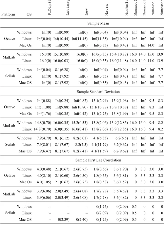
The univariate summary statistics we assessed are the sample mean, the sample
standard deviation and the sample first lag correlation of nine datasets (Table 1).
These datasets are classified by NIST in three levels of numerical difficulty:
low,
average
and
high. The datasets with low difficulty are
Lew,
Lottery,
Mavro,Michelso(these four datasets come from real world experiments),NumAcc1 andPiDigits. The average difficulty datasets areNumAcc2andNumAcc3, while NumAcc4is the only high difficulty dataset. The certified values were calculated using multiple precision arithmetic to obtain 500 digits answers.
The commandmeanis common to all platforms. The standard deviation in Octave and MatLab is computed with the commandstd, whereas the Scilab command is st_deviation. For computing the correlation, Scilab provides the functioncorrel which, surprisingly and in spite of what is informed in the documentation, returns the covariance rather than the correlation; the correlation was obtained dividing this result by the product of the sample standard deviations of the subvectors. In Octave we used the commandCorrel(v(1:n-1), v(2:n)), and in Matlab the command applied wascorr(v(1:n-1), v(2:n)), considering in both the vectorvof sizen≥3.
The values in parenthesis are the bootstrap estimates of the standard deviation of L R Es,sL R E. Whenever ‘Inf’ was observed, L R E = 16, i.e., the highest possible accuracy in double precision, was used.
3.2
Statistical functions
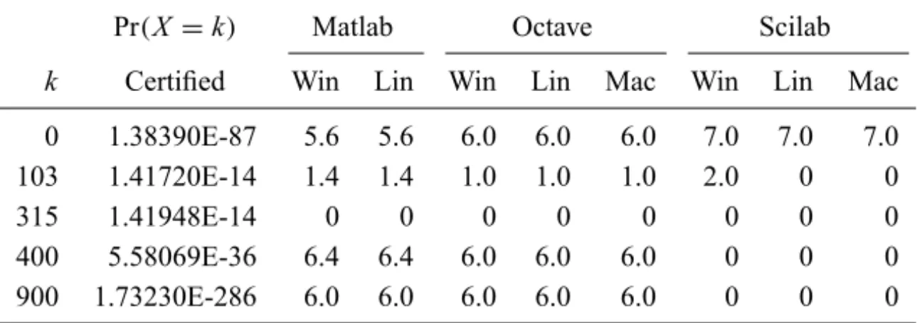
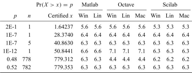
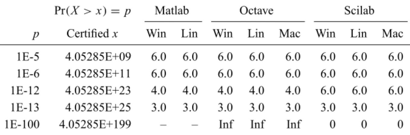
The distributions herein assessed are the binomial (Table 2), Poisson (Tables 3 and 4), gamma (Table 5), normal (Table 6),χ2(Table 7), beta (Table 8), t-Student (Table 9) and F(Table 10).
Platform OS Pi D i g i t s L o t t e r y L e w M a v r o M i c h e l s o N u m a c c 1 N u m a c c 2 N u m a c c 3 N u m a c c 4 Sample Mean Octave
Windows Inf(0) Inf(0.99) Inf(0) Inf(0.04) Inf(0.04) Inf Inf Inf Inf Linux Inf(0.04) Inf(10.44) Inf(11.45) Inf(11.35) Inf(10.94) Inf Inf Inf Inf Mac Os Inf(0) Inf(0.99) Inf(0) Inf(0.33) Inf(0.43) Inf Inf 14.0 Inf
MatLab Windows 16.0(0) 15.1(0.89) 16.0(0) 16.0(0.35) 15.4(10.87) 16.0 14.0 15.0 13.9 Linux 16.0(0) 16.0(0.03) 16.0(0) 16.0(0.35) 16.0(11.48) 16.0 14.0 14.0 13.9
Scilab
Windows Inf(0.04) 8.1(6.28) Inf(0) Inf(0.04) Inf(0.04) Inf Inf Inf 7.7 Linux Inf(0) 8.1(7.92) Inf(0) Inf(0.33) Inf(0.43) Inf Inf Inf 7.7 Mac OS Inf(0) 8.1(7.92) Inf(0) Inf(0.33) Inf(0.43) Inf Inf Inf 7.7
Sample Standard Deviation
Octave
Windows Inf(0.88) Inf(0.24) Inf(0.87) 13.1(2.94) 13.9(1.96) Inf Inf 9.5 8.3 Linux Inf(11.08) Inf(9.88) Inf(10.80) 13.1(10.88) 13.9(10.88) Inf Inf 8.3 Inf Mac Os Inf(1.76) Inf(0.35) Inf(0.42) 13.1(2.75) 13.8(1.99) Inf Inf 9.5 8.3
MatLab Windows 14.8(0.70) 16.0(0.35) 15.2(0.53) 13.8(2.06) 13.9(12.85) 16.0 16.0 9.4 8.2 Linux 14.8((0.70) 16.0(0.35) 16.0(0.41) 13.8(2.06) 13.9(12.85) 16.0 16.0 9.4 8.2
Scilab
Windows 7.9(4.79) 8.1(6.12) 8.2(6.01) 4.1(6.33) 6.2(6.5) Inf Inf Inf Inf Linux 7.9(8.01) 8.1(7.67) 8.2(7.5) 4.1(11.79) 6.2(9.62) Inf Inf Inf Inf Mac OS 7.9(6.47) 8.1(7.67) 8.2(7.41) 4.1(11.59) 6.2(9.62) Inf Inf Inf Inf
Sample First Lag Correlation
Octave
Windows 4.0(0.48) 2.1(0.67) 2.6(0.75) 1.8(0.56) 3.6(1.90) 0 3.0 3.0 3.0 Linux 4.0(2.10) 2.1(0.60) 2.6(0.50) 1.8(0.55) 3.6(1.81) 0 3.3 3.3 3.3 Mac Os 4.0(1.05) 2.1(0.67) 2.6(0.75) 1.8(0.58) 3.6(1.52) 0 3.0 3.0 3.0
MatLab Windows 3.9(6.06) 2.0(3.49) 2.6(4.08) 1.7(2.78) 3.5(4.82) 0 3.3 3.3 3.3 Linux 3.9(6.06) 2.0(3.49) 2.6(4.08) 1.7(2.78) 3.5(4.82) 0 3.3 3.3 3.3
Scilab
Windows – – – 0(1.75) 0(2.09) 0.5 0 0 0
Linux – – – 0(2.09) 0(2.09) 0.5 0 0 0
Mac OS – 0(2.39) 0(2.40) 0(1.75) 0(2.09) 0.5 0 0 0
Octave, while Matlab provides the commandbetainv. Scilab provides cdfbin, cdfpoi,cdfgam,cdfnor,cdfchi,cdfbet,cdftandcdfffor computing the binomial, Poisson, gamma, normal,χ2, beta, t-Student andFquantiles, respectively.
Pr(X≤k) Matlab Octave Scilab
k Certified Win Lin Win Lin Mac Win Lin Mac
1 8.96114E-308 3.0 3.0 0 0 0 Inf Inf Inf
2 4.61499E-305 3.0 3.0 0 0 0 8.0 8.0 8.0
100 1.39413E-169 1.0 1.0 0 0 0 7.0 7.0 7.0
300 2.91621E-42 0 0 0 0 0 7.0 7.0 7.0
400 3.89735E-13 0 0 0 4.0 4.0 6.0 6.0 6.0
410 3.19438E-11 0 0 0 6.0 6.0 6.0 6.0 6.0
Table 2 – Binomial distribution,n=1030 and p=1/2.
Pr(X =k) Matlab Octave Scilab
k Certified Win Lin Win Lin Mac Win Lin Mac
0 1.38390E-87 5.6 5.6 6.0 6.0 6.0 7.0 7.0 7.0
103 1.41720E-14 1.4 1.4 1.0 1.0 1.0 2.0 0 0
315 1.41948E-14 0 0 0 0 0 0 0 0
400 5.58069E-36 6.4 6.4 6.0 6.0 6.0 0 0 0
900 1.73230E-286 6.0 6.0 6.0 6.0 6.0 0 0 0
Table 3 – Poisson probabilities,λ=200.
3.3
Linear regression
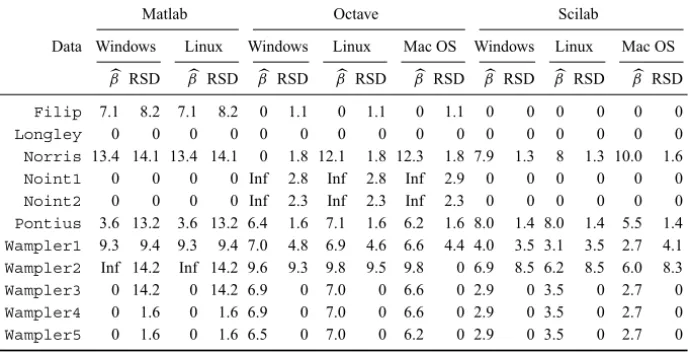
NIST offers eleven datasets to perform linear regression analysis. The datasets are divided into numerical difficulty levels: two of low level, (NorrisandPontius), two of average level, (Noint1andNoint2) and seven of high level. Table 11 presents the smallest LRE of each regression, and the LRE of the residual standard deviation (RSD) of each fit.
Pr(X ≤k) Matlab Octave Scilab
k λ Certified Win Lin Win Lin Mac Win Lin Mac
1E+05 1E+05 0.500841 1.0 1.0 1.0 1.2 1.0 7.0 7.0 7.0
1E+07 1E+07 0.500084 7.0 7.0 7.0 7.0 7.0 6.0 6.0 6.0
1E+09 1E+09 0.500008 7.0 7.0 7.0 7.0 7.0 6.0 6.0 6.0
Table 4 – Poisson distribution functions,λ=200.
Pr(X≤x) Matlab Octave Scilab
x α Certified Win Lin Win Lin Mac Win Lin Mac
0.1 0.1 0.827552 7.0 7.0 7.0 7.0 7.0 7.0 7.0 7.0
0.2 0.1 0.879420 6.0 6.0 6.0 6.0 6.0 6.0 6.0 6.0
0.2 0.2 0.764435 6.0 6.0 6.0 6.0 6.0 6.0 6.0 6.0
0.4 0.3 0.776381 6.0 6.0 6.0 6.0 6.0 6.0 6.0 6.0
0.5 0.4 0.748019 6.0 6.0 6.0 6.0 6.0 6.0 6.0 6.0
Table 5 – Gamma distribution functions,β =1.
Matlab Octave Scilab
p Certifiedzp Win Lin Win Lin Mac Win Lin Mac
5E-1 0 Inf Inf Inf Inf Inf 0 0 0
1E-198 -30.0529 7.0 7.0 7.0 7.0 7.0 3.0 3.0 3.0
1E-300 -37.0471 7.0 7.0 7.0 7.0 7.0 1.0 1.0 1.0
Table 6 – Normal quantiles,μ=0 andσ =1.
Pr(X >x)=p Matlab Octave Scilab
p n Certifiedx Win Lin Win Lin Mac Win Lin Mac
2E-1 1 1.64237 5.6 5.6 5.6 5.6 5.6 5.3 5.3 5.3
1E-7 1 28.3740 6.4 6.4 6.4 6.4 6.4 6.4 6.4 6.4
1E-7 5 40.8630 6.3 6.3 6.3 6.3 6.3 6.3 6.3 6.3
1E-12 1 50.8441 6.6 6.6 7.1 7.1 7.1 6.3 6.3 6.3
0.48 778 779.312 6.3 6.3 4.4 4.4 4.4 6.2 6.2 6.2
0.52 782 779.353 6.3 6.3 6.3 6.3 6.3 6.3 6.3 6.3
Matlab Octave Scilab
p Certified Win Lin Win Lin Mac Win Lin Mac
1E-2 2.94314E-01 6.0 6.0 6.0 6.0 6.0 6.0 6.0 6.0
1E-3 1.81386E-01 6.1 6.1 6.0 6.0 6.0 6.0 6.0 6.0
1E-4 1.12969E-01 5.4 5.4 5.0 5.0 5.0 5.0 5.0 5.0
1E-5 7.07371E-02 6.2 6.2 6.0 6.0 6.0 6.0 6.0 6.0
1E-6 4.44270E-02 6.0 6.0 6.0 6.0 6.0 6.0 6.0 6.0
1E-7 2.79523E-02 5.9 5.9 6.0 6.0 6.0 6.0 6.0 6.0
1E-8 1.76057E-02 6.3 6.3 6.0 6.0 6.0 6.0 6.0 6.0
1E-9 1.10963E-02 5.5 5.5 5.0 5.0 5.0 5.0 5.0 5.0
1E-10 6.99645E-03 6.7 6.7 7.0 7.0 7.0 7.0 7.0 7.0
1E-11 4.41255E-03 6.7 6.7 7.0 7.0 7.0 7.0 7.0 7.0
1E-12 2.78337E-03 5.9 5.9 6.0 6.0 6.0 6.0 6.0 6.0
1E-13 1.75589E-03 6.1 6.1 6.0 6.0 6.0 6.0 6.0 6.0
1E-100 6.98827E-21 6.8 6.8 7.0 0 0 7.0 7.0 7.0
Table 8 – Beta quantiles,α=5 andβ =2.
Pr(X >x)=p Matlab Octave Scilab
p Certifiedx Win Lin Win Lin Mac Win Lin Mac
1E-8 3.18310E+07 0 0 0 0 0 6.0 6.0 6.0
1E-11 3.18310E+10 0 0 0 0 0 6.0 6.0 6.0
1E-12 3.18310E+11 – – – – – 6.0 6.0 6.0
1E-13 3.18310E+12 0 0 0 0 0 6.0 6.0 6.0
1E-100 3.18310E+99 – – – – – 8.0 8.0 0
Table 9 – The t-Student distribution,n=1.
Pr(X >x)=p Matlab Octave Scilab
p Certifiedx Win Lin Win Lin Mac Win Lin Mac
1E-5 4.05285E+09 6.0 6.0 6.0 6.0 6.0 6.0 6.0 6.0
1E-6 4.05285E+11 6.0 6.0 6.0 6.0 6.0 6.0 6.0 6.0
1E-12 4.05285E+23 4.0 4.0 4.0 4.0 4.0 6.0 6.0 6.0
1E-13 4.05285E+25 3.0 3.0 3.0 3.0 3.0 3.0 3.0 3.0
1E-100 4.05285E+199 – – Inf Inf Inf 0 0 0
Matlab Octave Scilab
Data Windows Linux Windows Linux Mac OS Windows Linux Mac OS b
β RSD βbRSD βbRSD βbRSD bβ RSD bβ RSD bβ RSD bβ RSD
Filip 7.1 8.2 7.1 8.2 0 1.1 0 1.1 0 1.1 0 0 0 0 0 0
Longley 0 0 0 0 0 0 0 0 0 0 0 0 0 0 0 0
Norris 13.4 14.1 13.4 14.1 0 1.8 12.1 1.8 12.3 1.8 7.9 1.3 8 1.3 10.0 1.6 Noint1 0 0 0 0 Inf 2.8 Inf 2.8 Inf 2.9 0 0 0 0 0 0 Noint2 0 0 0 0 Inf 2.3 Inf 2.3 Inf 2.3 0 0 0 0 0 0 Pontius 3.6 13.2 3.6 13.2 6.4 1.6 7.1 1.6 6.2 1.6 8.0 1.4 8.0 1.4 5.5 1.4 Wampler1 9.3 9.4 9.3 9.4 7.0 4.8 6.9 4.6 6.6 4.4 4.0 3.5 3.1 3.5 2.7 4.1 Wampler2 Inf 14.2 Inf 14.2 9.6 9.3 9.8 9.5 9.8 0 6.9 8.5 6.2 8.5 6.0 8.3 Wampler3 0 14.2 0 14.2 6.9 0 7.0 0 6.6 0 2.9 0 3.5 0 2.7 0 Wampler4 0 1.6 0 1.6 6.9 0 7.0 0 6.6 0 2.9 0 3.5 0 2.7 0 Wampler5 0 1.6 0 1.6 6.5 0 7.0 0 6.2 0 2.9 0 3.5 0 2.7 0
Table 11 – LRE of linear regression results.
3.4
Results on decisions based on matrices
The commanddetis used by all three platforms under assessment to compute determi-nants. As proposed Section 2, the evaluation is based on comparing the results with the certified value zero, rather than on the numerical value itself. This is due to the fact that more often than not what users are interested upon is a decision, and not a numerical value.
Curiosily, the number of correct results of comparing|gM|with zero was the same, that is, exactly 146 for the three platforms under assessment.
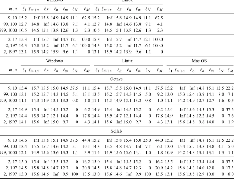
The results of computing spectral graph analyses are presented in Table 12.
4
Conclusions
Regarding the computation of basic statistics, Table 1 shows that the mean poses little difficulty for the platforms, with the exception of Octave for Linux, which presented the smallest number of LRE in five of the nine datasets (LRE(x,c)≤7). Surprisingly, these five datasets offer low numerical difficulty.
When computing the standard deviation, Octave presented the bests results when comparing with others two platforms. The version tested here was better than the one tested before (see [8]). Scilab presented an unacceptable low accuracy in a single dataset, for which LRE(x,c)≤5.
E L IA N A S . D E A L M E ID A , A N T O N IO C . M E D E IR O S and A L E JA N D R O C . F R E R Y 535
m,n ℓ1 ℓm+n ℓS ℓn ℓm ℓN ℓM ℓ1 ℓm+n ℓS ℓn ℓm ℓN ℓM
9,10 15.2 Inf 15.8 14.9 14.9 11.1 62.5 15.2 Inf 15.8 14.9 14.9 11.1 62.5 99,100 12.7 14.8 Inf 14.6 13.8 7.1 4.1 12.7 14.8 Inf 14.6 13.8 7.1 4.1 999,1000 10.5 14.5 15.1 13.8 12.6 1.3 2.3 10.5 14.5 15.1 13.8 12.6 1.3 2.3
2,17 15.3 Inf 15.7 Inf 14.7 12.1 100.0 15.3 Inf 15.7 Inf 14.7 12.1 100.0 2,197 14.3 15.8 15.2 inf 11.7 6.1 100.0 14.3 15.8 15.2 inf 11.7 6.1 100.0 2,1997 13.1 15.9 14.2 15.9 9.6 1.1 0 13.1 15.9 14.2 15.9 9.6 1.1 0
Windows Linux Mac OS
m,n ℓ1 ℓm+n ℓS ℓn ℓm ℓN ℓM ℓ1 ℓm+n ℓS ℓn ℓm ℓN ℓM ℓ1 ℓm+n ℓS ℓn ℓm ℓN ℓM
Octave
9,10 15.4 15.7 15.5 15.0 14.9 37.5 11.1 15.4 15.7 15.5 15.0 14.9 11.1 37.5 15.2 Inf Inf 14.8 15.1 12.5 22.2 99,100 13.1 15.2 15.7 14.3 14.5 5.1 13.1 13.5 15.2 15.7 14.3 14.5 5.0 9.2 13.0 15.3 15.4 13.9 14.1 8.0 7.1 999,1000 11.1 14.3 14.9 13.1 13.3 0.8 1.0 11.1 14.3 14.9 13.1 13.3 0.8 1.0 11.1 14.2 14.9 12.7 12.7 1.6 0.5
2,17 14.9 15.4 Inf 14.5 15.2 0 6.2 14.9 15.4 Inf 14.5 15.2 0 6.2 15.4 Inf 15.6 14.3 15.3 0 37.5 2,197 14.4 15.9 14.7 12.1 14.4 0 17.8 14.4 15.9 14.7 12.1 14.4 0 17.8 14.9 Inf 14.8 12.2 14.5 0 7.6 2,1997 14.1 15.6 Inf 15.0 9.7 0 4.3 14.1 15.6 Inf 15.0 9.7 0 4.3 13.1 15.6 14.8 9.6 14.0 0 1.9
Scilab
9,10 14.6 Inf 15.8 15.1 14.9 37.5 44.4 15.2 Inf 15.8 15.4 15.0 25.0 44.0 15.2 Inf Inf 14.8 15.1 12.5 22.2 99,100 13.4 15.5 15.7 14.6 14.2 5.1 10.1 14.3 15.5 14.8 14.7 Inf 7.1 6.1 13.0 15.4 15.7 13.8 13.8 4.1 5.0 999,1000 12.1 14.9 15.6 13.6 13.3 1.1 3.9 11.4 14.9 15.6 13.6 14.1 1.0 1.8 10.9 14.2 14.8 13.1 13.1 1.3 1.1
2,17 15.0 15.4 Inf 15.5 15.2 0 16.2 15.0 15.4 Inf 15.5 15.2 0 16.2 15.5 Inf 15.7 15.4 14.4 0 37.5 2,197 14.5 15.8 14.8 14.7 12.3 0 20.9 14.5 15.8 14.8 14.7 12.3 0 20.9 14.2 15.6 14.3 14.0 12.0 0 17.3 2,1997 13.0 15.6 14.6 Inf 9.9 100 13.5 13.0 15.6 14.6 Inf 9.9 100 13.5 13.1 15.6 13.5 12.9 10.0 0 8.0
Table 12 – Accuracy computing spectral graph analyses.
Scilab is also the worst platform with respect to the stability of the results, as measured by estimated standard variation of the observedL R E. As can be noted in Table 1, all conclusions about the standard deviation may be reverted with small perturbations of the original input, e.g., the best results which were produced for theLewdataset can be turned into unacceptable by subtractingsL R Efrom the observed L R E.
Two other cases are notorious for their instability: the sample mean and the sample standard deviation, both computed by Octave under Linux. In most of the other cases, small perturbations of the original input do not change the conclusion about the precision. Scilab presented the best performance when dealing with the binomial and t-Student distributions, and also when computing the cumulative distribution function of the Pois-son law (LRE(x,c)≥6). In this last, Octave and MatLab presented better results that their previous versions (see [8]).
When computing the F distributions, Octave produced the best results, mainly if compared with its previous version; as presented by Frery et al. [8], this platform had produced the worst answers. But Octave fails to produce acceptable results when deal-ing with the binomial and t-Student laws. Regarddeal-ing the normal distribution, MatLab and Octave obtained the same good results, while Scilab produced bad results. The three platforms were acceptable when dealing with the gamma law, that is, in this case LRE(x,c)≥6.
Matlab and Octave failed at computing the t-Student distribution; in every assessed case, there was no match or they returned an error message. This is a serious issue due to the widely spread use of this distribution in statistical tests.
Six out of eleven linear regression datasets were not adequately dealt with by any of the considered platforms. Only Matlab provided acceptable results forFilip,Norris, Wampler1and forWampler2.Wampler2was acceptably treated by Octave under Windows and Linux and Scilab under the three operational systems. Again, no single platform can be advised as safe for the linear regression problems here considered.
Suprisingly, the same results were provided by the three platforms when making decisions about the determinant of ill-conditioned matrices under the three operating systems. The number of erroneus result was acceptable, that is only 94 in 240 logical comparisons with the value zero. Nevertheless, users are advised to be very careful when testing equality between a value of interest and a numerical computation involving determinats in these platforms.
The assessment based on spectral graph analysis presented a very consistent behavior with respect to the problem size (the bigger the graph, the worse the answer), being
precision, being the latter consistently more precise than the former. The balance of bipartite connected graphs did not have a strong impact on the results, except for the percentage of correct eigenvalues.
Extreme care must be taken when making decisions about graphs based on their spectral properties. As a rule of the thumb, double-precision computation is advised, but the comparison to known values should be made rounding or, at most, using at most floating point representation.
Regarding the variability among operating systems, MatLab and Octave were equiv-alent and more consistent than Scilab in most of the situations under assessment.
The results are the same in platforms under 32 and 64 bits operating systems, so the latter were not reported in the tables.
REFERENCES
[1] M. Al-Nasra and D.T. Nguyen,An algorithm for domain decomposition in finite element analisys.Computers & Structures (1991).
[2] M. Almiron, B.L. Vieira, A.L.C. Oliveira, A.C. Medeiros and A.C. Frery,On the numerical accuracy of spreadsheets.Journal of Statistical Software,34(4) (2010), 1–29.
[3] M.G. Almiron, E.S. Almeida and M.N. Miranda,The reliability of statistical func-tions in four software packages freely used in numerical computation.Brazilian Journal of Probability and Statistics,23(2) (2009), 107–119.
[4] M.G. Almiron, B. Lopes, A.L.C. Oliveira, A.C. Medeiros and A.C. Frery,On the numerical accuracy of spreadsheets. Journal of Statistical Software,34(4) (2010), 1–29.
[5] B. Bollobas,Modern Graph Theory. Springer (1998).
[6] O.H. Bustos and A.C. Frery,Statistical functions and procedures in IDL 5.6 and 6.0.Computational Statistics & Data Analysis,50(2), 301–310, January (2006). [7] M. Fiedler,Algebraic connectivity of graphs.Czechoslovak Mathematical Journal,
23(98) (1973), 298–305.
[9] K.B. Keeling and R.J. Pavur,A comparative study of the reliability of nine statis-tical software packages.Computational Statistics & Data Analysis,51(8), 3811– 3831, May (2007).
[10] B.D. McCullough,Assessing the reliability of statistical software: Part I.American Statistician,52(4), 358–366, November (1998).
[11] B.D. McCullough and B. Wilson,On the accuracy of statistical procedures in Microsoft Excel 97.Computational Statistics & Data Analysis,31(1), 27–37, July (1999).
[12] B.D. McCullough and B. Wilson,On the accuracy of statistical procedures in Microsoft Excel 2000 and Excel XP.Computational Statistics & Data Analysis,
40(4), 713–721, October (2002).
[13] B.D. McCullough and B. Wilson,On the accuracy of statistical procedures in Microsoft Excel 2003.Computational Statistics & Data Analysis, 49(4), 1244– 1252, June (2005).
[14] B.D. McCulluogh,The accurary of Mathematica 4 as a statistical package. Com-putational Statistics,15(2) (2000), 279–299.
[15] National Institute of Standards and Technology, Statistical reference datasets, 2010. URL http://www.itl.nist.gov/div898/strd/general/dataarchive.html.