IMPROVED
H
2AND
H
∞CONDITIONS FOR ROBUST ANALYSIS AND
CONTROL SYNTHESIS OF LINEAR SYSTEMS
Alexandre Trofino
∗Daniel F. Coutinho
†Karina A. Barbosa
‡∗Dept. Automation and Systems, UFSC, PO Box 476, 88040-900, Florianópolis, SC, Brazil.
†Dept. Electrical Engineering, PUCRS, Av. Ipiranga 6681, 90619-900, Porto Alegre, RS, Brazil.
‡Dept. of Systems and Control, LNCC/MCT, Av. Getúlio Vargas 333, 25651-070, Petrópolis, RJ, Brazil
ABSTRACT
This paper proposes improved H-2 and H-infinity conditions for continuous-time linear systems with polytopic uncertain-ties based on a recent result for the discrete-time case. Basi-cally, the performance conditions are built on an augmented-space with additional multipliers resulting in a decoupling between the Lyapunov and system matrices. This nice prop-erty is used to develop new conditions for the robust stability, performance analysis, and control synthesis of linear systems using parameter dependent Lyapunov functions in a numeri-cal tractable way.
KEYWORDS: Robustness, H2/H∞ norms, convex opti-mization.
RESUMO
Este artigo propõe novas condições para as normas 2 e H-infinito para sistemas lineares incertos utilizando as idéias originalmente propostas para sistemas discretos. Basica-mente, as condições de desempenho são obtidas em espaço de estados aumentado onde novas variáveis livres são
adi-ARTIGO CONVIDADO:
Versão completa e revisada de artigo apresentado no CBA-2004 Artigo submetido em 15/12/04
1a. Revisão em 21/06/05
Aceito sob recomendação do Ed. Assoc. Prof. Liu Hsu
cionadas ao problema resultando em uma separação entre as matrizes do sistema e de Lyapunov. Este propriedade é utilizada no desenvolvimento de novos critérios para análise de estabilidade robusta e desempenho, e síntese de controle para sistemas lineares utilizando funções de Lyapunov de-pendente de parâmetros que podem ser resolvidas através de problemas de otimização convexa.
PALAVRAS-CHAVE: Robustez, normasH2eH∞, otimiza-ção convexa.
1
INTRODUCTION
discrete-time systems. In other words, the following usual condition
A′P A−P <0 (1) is replaced by the following improved condition
P+G+G′ A′G′
GA −P
<0. (2)
Notice that the termA′P Ain (1) is the main source of con-servativeness when dealing with uncertain system and robust design with mixed performance specifications. The reason is that robust performance tests are less conservative when
Pis parameterized in terms of the uncertainties and the per-formance indexes, but the robust controller parametrization requires a singleP to be used. The improved condition in (2) eliminates the constraint of a single Lyapunov function because the controller parametrization does not depend on
P.
Since the publication of the aforementioned paper, several researchers have tried to get a similar result for linear contin-uous time systems. However, the proposed results are not convex, as for instance the techniques in (Shaked, 2001), (Trofino and de Souza, 2002), and even the convex approach proposed by Apkarian et al. (2001) has shown to be more conservative than the usual quadratic stability test in many cases. At the same time, Ebihara and Hagiwara (2002) have proposed a dilated LMI version of the standard LMI tests for robust control synthesis under mixed performance spec-ifications by means of parameter-dependent Lyapunov func-tions. As in the previous references, the method is not convex when solving robust control problems because a scalar must be tuned using a line search procedure. Some nice properties of this line search problem are presented in the paper.
From the above scenario, this paper aims to present new LMI conditions forH2andH∞analysis of linear uncertain con-tinuous time systems. Similarly to Apkarian et al. (2001) and (Ebihara and Hagiwara, 2002), the proposed approach is convex but in some cases may be more conservative than the usual LMI conditions based on quadratic stability, this behavior relies on the fact that the dilated conditions only re-cover the standard LMI quadratic stability tests for the nom-inal case. A strong argument to use the improved conditions instead of the usual LMI tests is its application for designing robust controllers with parameter-dependent Lyapunov func-tions consideringH2orH∞specifications and even mixed performance criteria. Aiming to stress that the proposed re-sults can lead to less conservative upper bounds of the per-formance criteria for uncertain systems, this paper focus on the performance analysis and the results illustrated through exhaustive numerical tests. Basically, the numerical experi-ments reported in Section 6 reveals that over 16000 randomly generated systems the proposed methodology has achieved a
better result in about83%of cases in the robustH2 norm against the usual quadratic stability tests and the approach of Apkarian et al. (2001) that surprisingly has got a better result for only one system. The results for the H∞ norm of uncertain systems are yet conservative and require further improvements. Section 7 presents the control results for both
H2andH∞performance specifications.
Notation. The notation used throughout this paper is stan-dard. Rn denotes the set of n-dimensional real vectors, Rn×m is the set of n×m real matrices, I
n is the n×n
identity matrix,0n is then×nmatrix of zeros. For a real
matrixS,S′denotes its transpose, andS >0means thatS is symmetric and positive-definite. The symbol⋆for a block matrix represents its symmetrical block outside the main di-agonal. Matrix and vector dimensions are omitted whenever they can be inferred from the context.
2
PROBLEM STATEMENT
Consider the following time-invariant system
S:
˙
x = Ax+Bw,
z = Cx+Dw, (3)
wherex ∈ Rn denotes the state,w ∈ Rm the disturbance
input vector, z ∈ Rq the performance vector, A, B, C, D
are real matrices of compatible dimensions. To represent some system dynamics and parameters that are not precisely known or are difficult to be exactly modelled, suppose the matrices of the systemScan take any value in a given poly-topeΠas indicated below (Boyd et al., 1994):
Π =Co
Ai Bi Ci Di
, i= 1, . . . , p
(4)
whereCo{·}refers to the convex hull of {·}. For
conve-nience, we may alternatively represent the uncertain system
Sby the notationS ∈Swhere the setSis as follows:
S :=
Sin (3):
A B C D
∈Π
(5)
One can characterize the system performance in terms of input-to-output experiments by means of the H2 and H∞ norms. When the disturbance signal is impulsive, theH 2-norm is the most indicated (assuming that D = 0), on the contrary for square integrable signals theL2-gain of the input-to-output operator (or simplyH∞-norm) can be used. For completeness, we provide the following definitions of system norms.
Definition 1 TheH2-norm of systemSis given by
kSk2,sup S∈S
m
X
i=1
wherez¯i(t)is the system response to a unitary impulse in the i−thinput channel withx(0) = 0andD= 0.
If the disturbance signalw(t)is a white noise with zero mean value and unitary power density spectra, theH2-norm may be interpreted as follows
kSk2 2,sup
S∈S
ε
(z(t)′z(t))where
ε
(z(t)′z(t))denotes the mathematical expectation ofthe random variablez(t)′z(t).
Alternatively, supposingx(0) = 0, the greatest energy gain that can be obtained from the disturbance signalw(t)∈ L2to the outputz(t)corresponds to theH∞-norm of the uncertain systemSleading to the following definition.
Definition 2 TheH∞-norm of systemSis given by
kSk∞, sup
S ∈S, 06=w∈ L2
kz(t)k2
kw(t)k2
(7)
whereL2denotes the space of square integrable vector func-tions on[0,∞).
From the above scenario, the problem to be addressed in this paper is to obtain a new set of less conservative LMI condi-tions to compute theH2andH∞system norms in a numeri-cal tractable way.
3
H
2ANALYSIS
Assuming thatD = 0, a bound on theH2-norm of system
S can be computed by the following standard result from the LMI theory and the observability Gramian (Boyd et al., 1994).
Lemma 1 Consider systemSwithD= 0. Suppose there ex-ist symmetric matricesPandNwith appropriate dimensions satisfying the follow optimization problem for allS ∈S.
min
P,Ntrace(N) :
P >0, N−B′P B >0,
A′P+P A+C′C <0. (8)
Then,Sis quadratically stable and the following holds:
kSk2
2<trace(N), ∀ S ∈S. (9)
From above, notice that the decision variableP multiplies the system matrix, and whenAis an affine function of an-other decision variable, as for instance the control-gainKin design control problems, Lemma 1 can be easily applied for
control design if the system matrices are perfectly known. However, for the class of systems considered in this paper a robust controller can be obtained only by considering a sin-gle Lyapunov matrixP (Shaked, 2001) which may be very conservative. To overcome this problem, an augmented-LMI version of Lemma 1 is proposed in the following.
Theorem 2 Consider systemS withD = 0. Suppose there exist positive definite matricesW, N and a free matrixG, with appropriate dimensions, satisfying the following opti-mization problem for allS ∈S.
min
W,N,Gtrace(N) :
N B′G′
GB W
>0,
W+ ˜A′G′+GA˜ Aˆ′G′ C′
GAˆ −W 0 C 0 −Iq
2
<0.
(10)
whereAˆ=A+InandA˜=A−In.
Then,Sis quadratically stable and the following holds:
kSk2
2<trace(N), ∀ S ∈S. (11)
Proof: Suppose there existW, G, N such that optimization problem (10) is satisfied.
Applying the Schur complement to the first LMI of (10) leads to
N−B′G′W−1
GB >0
Now, defining the Lyapunov matrix as
P,G′W−1
G, (12) we getN−B′P B >0.
Consider the second LMI of (10) and applying the Schur complement yields
ˆ
A′G′W−1
GAˆ+ (W + ˜A′G′+GA) + 2C˜ ′C <0. (13) From the fact that1
W+ ˜A′G′+GA˜+ ˜A′G′W−1
GA˜≥0,
condition (13) implies
ˆ
A′PAˆ−A˜′PA˜+ 2C′C= 2(A′P+P A+C′C)<0 taking into account the definition ofPin (12).
Finally, the rest of the proof follows from Lemma 1. ✷
Remark 1 The advantage of considering Theorem 2 instead of Lemma 1 is obvious for polytopic systems, since we can employ parameter-dependent Lyapunov matrices in Theorem 2 by only considering thatW = Wi (fori = 1, . . . , p) in
(10).
4
H
∞ANALYSIS
From the following LMI version of the Bounded Real Lemma (Boyd et al., 1994), an upper bound on theH∞-norm of systemScan be determined.
Lemma 3 Consider system S. Suppose there exist a sym-metric matrixP with appropriate dimension and a scalarγ
satisfying the follow optimization problem for allS ∈S.
min
P γ: P >0,
A′P+P A P B C′
B′P −γI m D′ C D −γIq
<0.
(14)
Then,Sis quadratically stable and the following holds:
kSk∞< γ,∀ S ∈S. (15)
From the same arguments of Section 3, the above Lemma may be conservative for control design of polytopic systems and also for multi-objective performance criteria (Apkarian et al., 2001). To overcome this problem, we give the follow-ing improvedH∞condition.
Theorem 4 Consider system S and suppose there exist a positive definite matrixW, a free matrixG and a positive scalarγsatisfying the following optimization problem for all
S ∈S.
min
W,G,γγ: W >0,
WG GB Aˆ′G′ 0 C′ B′G′ −2γI
m B′G′ 0 D′ GAˆ GB −W 0 0
0 0 0 −2γIm 0
C D 0 0 −γ2Iq
<0
(16)
whereWG=W+GA˜+ ˜A′G′,Aˆ=A+InandA˜=A−In.
Then,Sis quadratically stable and the following holds:
kSk∞< γ,∀ S ∈S. (17)
Proof: Suppose that Theorem 4 is satisfied. Also, for conve-nience, define the following notation:
Wa=
W 0 0 2γIm
, Ga=
G 0 0 γIm
ˆ Aa=
ˆ
A B 0 0m
, A˜a=
˜
A B 0 −2Im
,
Aa=
A B 0 −Im
, Ca = C D ,
Pa =G′aW−
1
a Ga =
P 0 0 γ2Im
(18)
From above, notice that we can recast (16) as follows
Wa+GaA˜a+ ˜A′aG′a Aˆ′aG′a Ca′ GaAˆa −Wa 0
Ca 0 −γ2Iq
<0
From Theorem 2, the above implies the following
A′
aPa+PaAa+ 1 γC
′ aCa<0
Finally, the above LMI is equivalent to (14) and the rest of
this proof follows from Lemma 3. ✷
Observe that the 4-th row and column of (16) can be re-moved, without loss of generality, reducing the size of the LMI.
Remark 2 From the same arguments of Remark 1, the improvement of Theorem 4 over the standard Bounded Real Lemma (BRL) is clear when we consider parameter-dependent Lyapunov matrices by takingW = Wi (fori = 1, . . . , p) in (16).
5
CONSERVATIVENESS
To show the source of conservativeness of the proposed method, consider the following identity:
Φ := 2(A′P+P A) = ˆA′PAˆ−A˜′PA.˜ (19) Without loss of generality let us decompose P as P = G′W−1G
for some free matrixGand someW >0to get
Φ = Aˆ′G′W−1
GAˆ−A˜′G′W−1
GA˜ (20)
≤ Aˆ′G′W−1
GAˆ+ ˜A′G′+GA˜+W (21) Using the last inequality as an upper bound for2(A′P+P A) we get the following LMI with the Schur complement
˜
A′G′+GA˜+W Aˆ′G′
GAˆ −W
<0 (22)
Clearly (22) implies Φ < 0. However, the converse is not true in general. An exception occurs when the choiceG = −WA˜−1
is possible. In this case we get
−W −Aˆ′( ˜A′)−1
W −WA˜−1Aˆ −W
<0 (23)
which in turn yields
ˆ
A′PAˆ−A˜′PA˜= 2(A′P+P A)<0
The choices G = −WA˜−1
and P = ( ˜A′)−1WA˜−1 are possible whenever the matrix A is not uncertain, because otherwiseP, G will depend on the same uncertain parame-ters leading (22) to be non-convex in these parameparame-ters. This shows that (22) is equivalent to the usual LMI quadratic sta-bility testΦ <0in the nominal case but it may be conser-vative in the uncertain case. The same conclusion follows from the results in Section 3, i.e. they may be conservative in the uncertain case but not in the nominal case. However, due to the particular structure of the matrices in (18) the re-lationGa =−WaA˜−a1is no longer possible which suggests
the results in section 4 may have an additional degree of con-servatism. This point needs further investigation.
6
NUMERICAL EXAMPLES
This section reports a conservativeness analysis of the pro-posed improved conditions by means of exhaustive tests over 16000 linear uncertain systems which are randomly gener-ated using Gaussian distribution with zero mean and unitary variance. Let us start with the results from Theorem 2. For each systemS, the robustH2norm is compute by:
(i) Theorem 2 with parameter-dependent Lyapunov func-tions (see Remark 1), refereed to as (N);
(ii) The approach of Apkarian et al. (2001), refereed to as (T);
(iii) The standard H2-norm computation of Lemma 1 (quadratic stability approach) which is referred to as (Q).
The robust methods to compute theH2-norm can be applied whenever the underlying system is robustly stable. In this sense, it is required the Hurwitz stability of each matrixA
generated from the convex combination ofA1, . . . , Apto
nu-merically verify kSk2 by means of a fine grid procedure. In addition, whenever necessary, we have to modifyA so that the Hurwitz stability is guaranteed for all A ∈ ΠA ,
Co{A1, . . . , Ap}. To minimize the computational burden,
such procedure has been applied only to the extreme values ofA. Specifically, whenever the randomly generated matrix
Aiis not Hurwitz stable,(σ+ 1)Inhas been subtracted from Ai, whereσis the maximum real part of the eigenvalues of Ai. Although the later procedure cannot ensure the Hurwitz
stability ofAoverΠA, it can significantly reduce the number
of generated systems that are not asymptotically stable over
ΠA.
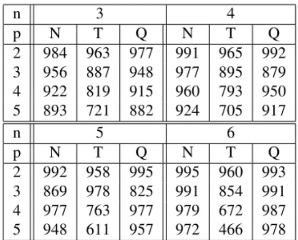
To carry out the statistical tests, we assume four different val-ues fornandpwhich are respectively the state vector dimen-sion and the vertex number. Precisely, we have taken 1000
n 3 4
p N T Q N T Q
2 984 963 977 991 965 992
3 956 887 948 977 895 879
4 922 819 915 960 793 950
5 893 721 882 924 705 917
n 5 6
p N T Q N T Q
2 992 958 995 995 960 993
3 869 978 825 991 854 991
4 977 763 977 979 672 987
5 948 611 957 972 466 978
Table 1: Number of systems for which the methods success-fully found a solution for theH2case
systems for each situationn = 3, . . . ,6andp = 2, . . . ,5, and our attention is focused on comparing:
(a) The number of times that each method provides a feasi-ble solution; and
(b) The number of times that each method achieve the best performance.
Table 1 shows the number of systems that lead to feasible solutions to the methods (N), (T) and (Q). Observe that, the new method (N) and the approach (Q) present similar num-ber of feasible solutions. Moreover, one can note that the approach (T) has worse performance.
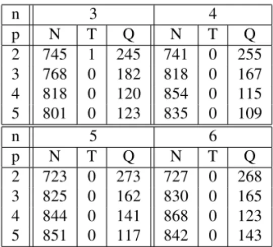
Table 2 shows the number of systems in which the ap-proaches (N), (T) and (Q) achieved the lowest upper-bound onkSk2. It turns out that the proposed H2 condition has achieved the best performance in a large majority of cases, and the improvement is even better with the increasing of the number of vertices, even though the standard quadratic stability test demonstrates a better performance in some sit-uations. In addition, the methodology proposed by Apkar-ian et al. (2001) has outperformed our approach and the quadratic method for only one system.
A similar study is now carried out to analyze the conserva-tiveness of the proposedH∞condition. To this end we solve the robustH∞problem by using the following approaches:
(i) Theorem 4 with parameter-dependent Lyapunov func-tions, refereed to as (N∞);
n 3 4
p N T Q N T Q
2 745 1 245 741 0 255
3 768 0 182 818 0 167
4 818 0 120 854 0 115
5 801 0 123 835 0 109
n 5 6
p N T Q N T Q
2 723 0 273 727 0 268
3 825 0 162 830 0 165
4 844 0 141 868 0 123
5 851 0 117 842 0 143
Table 2: The number of systems corresponding to the ap-proach achieving the lowest bound onkSk2.
To the authors’ knowledge, there is no other convex approach to robustH∞-norm computation in the continuous-time con-text.
Assumingn= 5,p= 3the number of feasible solution over 1000 systems are985with the proposed method (N∞) and
986with the usual method (Q∞). The quadratic approach (Q∞) has achieved the best performance in 542 cases, and the new approach (N∞) in303cases. The sameH∞upper bound was obtained with both methods in 141 cases. The sit-uation is similar for other values ofpandn. These numerical experiments confirm the claim in the previous section that the results forH∞are yet conservative and need to be improved.
7
STATE-FEEDBACK CONTROL
One of the most advantages of the proposedH2 and H∞ conditions is the possibility of designing a robust state-feedback control law considering parameter-dependent Lya-punov functions. Notice that convex conditions for control design can be easily obtained from the Dual version of The-orems 2 and 4. To extend these theThe-orems for control design, considerSas defined in (3) with an additional control input
u(t)∈Rr, i.e.:
S:
˙
x = Ax+Bw+Eu, z = Cx+Dw+F u, u = Kx,
(25)
where K ∈ Rr×n is the control-gain to be determined, E ∈ Rn×r, andF ∈ Rq×r are uncertain matrices.
Simi-larly to Section 2, the uncertain systemS is represented by the notationS ∈S, where the setSis redefined accordingly
to (25).
7.1
H
2Design
Setting D = 0, a state-feedback control law that stabilizes systemS(while minimizing an upper-bound on itsH2-norm for allS ∈S) can be obtained by means of the dual version
of Theorem 2.
The dual version of the improved H2 condition is de-vised from the controllability Gramian (Green and Lime-beer, 1995) leading to the following result.
Theorem 5 Consider systemS withD = 0. Suppose there exist symmetric matrices Wi, N (i = 1, . . . , p), and
non-symmetric onesG, Y with appropriate dimensions satisfying the following optimization problem for allS ∈S.
min Wi,N,G,Y
trace(N) :
N CG+F Y ⋆ Wi
>0,
Wi+ ˜AG+G′A˜′ +EY +Y′E′
⋆ ⋆
G′Aˆ′+Y′E′ −W i 0 B′ 0 −Im
2 <0. (26)
wherei= 1, . . . , p.
Then,Sis asymptotically stable with
u(t) =Y G−1
x(t),
andkSk2satisfies (11) for allS ∈S.
Proof: The proof of above Theorem is straightforward from the controllability Gramian and the control parametrization
Y =KG. ✷
Example 1 Consider a mass/spring/damper system given by the following representation (Zhou, 1998):
˙
x=A(k1, k2)x+Bw+Eu, z=Cx+F u, (27) where x = [ x1 x2 x3 x4 ]′, k1 ∈ [ 0.8,1.2 ],
k2 ∈ [ 3.2,4.8 ], and
A=
0 0 1 0
0 0 0 1
−k1 k1 −0.2 0.2
k1
2 −
k1+k2
2 0.1 −0.15
, B=
0 0 0 0.5 , E= 0 0 1 0 , C=
1 0 0 0 0 0 0 0
, F= 0 1 .
Applying Theorem 5, we get an upper-bound on the system 2-norm (in closed-loop) ofλ= 0.3478with a control matrix
K=−
0.4839 0.2348 0.6042 0.2929
It turns out that our approach has lead to a better result than the one proposed in (Apkarian et al., 2001) which get an upper-bound ofλ= 0.3959.
7.2
H
∞Design
Similarly to theH2case, one can obtain a (robust) stabiliz-ing state-feedback controller such that an upper-bound on the
H∞-norm ofS is minimized by means of a dual version of Theorem 4.
Basically, we redefine the BRL in terms of the Lyapunov ma-trix inverse and then apply standard results from the mama-trix theory. These manipulations yields the following result.
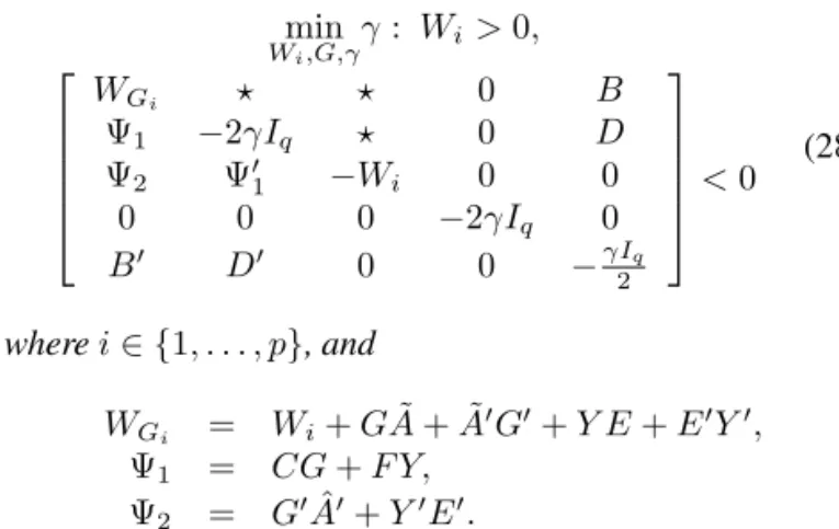
Theorem 6 Consider systemSand suppose there exist sym-metric matricesW1, . . . , Wp, non-symmetric ones,GandY,
and a positive scalarγsatisfying the following optimization problem for allS ∈S.
min Wi,G,γ
γ: Wi>0,
WGi ⋆ ⋆ 0 B
Ψ1 −2γIq ⋆ 0 D
Ψ2 Ψ′1 −Wi 0 0
0 0 0 −2γIq 0
B′ D′ 0 0 −γIq 2
<0 (28)
wherei∈ {1, . . . , p}, and
WGi = Wi+GA˜+ ˜A
′G′+Y E+E′Y′,
Ψ1 = CG+F Y,
Ψ2 = G′Aˆ′+Y′E′.
Then,Sis asymptotically stable with
u(t) = Y G−1
x(t),
and (17) is satisfied for allS ∈S.
Proof: The proof of above Theorem is straightforward from the dual version of Theorem 4, i.e., by setting P = P−1, G = G−1, A = A′, B = C′ andC = B′, and then applying the control parametrizationY =KG. ✷
Example 2 Consider the following linear time-invariant sys-tem borrowed from (Gahinet et al., 1994):
˙ x=
0 0 1 0
0 0 0 1
−k k −f f
k −k f −f
x+
0 0 0 0 0 1 1 0
w u
,
z=
0 1 0 0 0 0 0 0
x+
0 0.01
u
Approach BRL Shaked Proposed
γ 1.557 1.478 1.498
Table 3: Comparative closed-loopH∞-norms.
wherex = [ x1 x2 x3 x4 ]′, k ∈ [ 0.09,0.4 ], and
f ∈[ 0.0038,0.04 ].
The problem to be addressed is to design a state-feedback law u = Kx such that the closed-loop system is robustly stable while minimizing an upper-bound on the worst-case
H∞-norm of the above system.
Applying Theorem 6, we get an upper-boundγ= 1.498with a control-gain given by
K=−
51.523 399.593 22.331 664.714
.
Table 3 shows a comparative study among the standard Bounded Real Lemma (BRL) in (Boyd et al., 1994), the im-proved LMI test of (Shaked, 2001, Lemma 3.1), and our ap-proach. In spite of the fact that our approach seems to be more conservative than the Shaked’s one, we stress the fact that our approach is convex while in (Shaked, 2001) a param-eterǫhas to be optimized.
8
CONCLUDING REMARKS
This paper have proposed improvedH2andH∞conditions for continuous-time linear systems with polytopic uncertain-ties. Basically, the performance conditions are built on an augmented-space with additional multipliers resulting in a decoupling between the Lyapunov and system matrices. This nice property can be used to design robust state-feedback controllers with parameter dependent Lyapunov functions taking into account bothH2 andH∞norms. Statistical nu-merical tests have proven the advantage of the proposedH2 approach over previous results from the robust control liter-ature. In addition, we have presented theH2andH∞ con-ditions for state-feedback design also considering parameter-dependent Lyapunov functions and a robust control law. Fu-ture research will concentrate on improving theH∞results that are yet conservative and extend the results for filtering and control problems.
ACKNOWLEDGMENTS
REFERENCES
Apkarian, P., Tuan, H. D. and Bernussou, J. (2001). Continuous-Time Analysis, Eigenstructure Assign-ment, andH2Synthesis With Enhanced Linear Matrix Inequality (LMI) Characterizations,IEEE Transactions on Automatic Control46(12): 1941–1946.
Boyd, S., Ghaoui, L. E., Feron, E. and Balakrishnan, V. (1994). Linear matrix inequalities in systems and con-trol theory, SIAM books.
de Oliveira, M. C., Bernussou, J. and Geromel, J. C. (1999). A New Discrete-Time Robust Stability Condition, Sys-tem & Control Letters37: 261–265.
Ebihara, Y. and Hagiwara, T. (2002). Robust Controller Synthesis with Parameter-Dependent Lyapunov Vari-ables: A Dilated LMI Approach, Proceedings of the 41st IEEE Conference on Decision and Control, Las Vegas, pp. 4179–4184.
Gahinet, P., Nemirovskii, A., Laub, A. J. and Chilali, M. (1994).LMI Control Toolbox, The Mathworks Inc.
Green, M. and Limebeer, D. J. N. (1995). Linear Robust Control, Prentice Hall.
Shaked, U. (2001). Improved LMI Representations for the Analysis and the Design of Continuous-Time Systems with Polytopic Type Uncertainty,IEEE Transactions on Automatic Control46(4): 652–656.
Trofino, A. and de Souza, C. E. (2002). H2 Control of Rational Parameter-Dependent Continuous-Time Sys-tems: A Parametric Lyapunov Function Approach, Pro-ceedings of the 15th IFAC World Congress, Barcelona, Spain, pp. 2344–2349.