Ariel Fraidenraich
Departamento de Matemática Facultad de Ingeniería Universidad de Buenos Aires Av. Paseo Colón 850 1063 Buenos Aires. Argentina afraide@ fi.uba.ar
Pablo M. Jacovkis
Departamento de Matemática Facultad de Ingeniería Universidad de Buenos Aires Departamento de Computación Universidad de Buenos Aires Ciudad Universitaria 1428 Buenos Aires. Argentina [email protected]
Fernando Roberto de A. Lima
Centro Regional de Ciências Nucleares Comissão Nacional de Energia Nuclear Av. Prof. Luiz Freire, 200 Cidade Universitária 50740-540 Recife, PE, Brazil [email protected]
Sensitivity Analysis of Shallow Water
Problems via Perturbative Methods
We applied the perturbative theory to perform sensitivity analysis of the shallow water equations. The numerical solution of these equations was found via the mass lumping finite element technique. Then, the adjoint system of the shallow water equations was derived for the one-dimensional case and the expression of the sensitivity coefficient of a generic functional with respect to a generic parameter (Chézy resistance coefficient, solitary wave amplitude and bed channel slope) was obtained, using the differential formalism. The sensitivity of the mean functional, representing the first approximation of the velocity and the depth, was analyzed with regard to these parameters. Results of the sensitivity coefficients obtained via the perturbative methodology satisfactorily matched the values computed by the direct method, i.e., by means of the direct solution of the shallow water equations changing the values of input parameters for each case considered.
Keywords: Sensitivity analysis, shallow water equations, perturbative methods, mass lumping technique
Introduction
The one-dimensional unsteady shallow water open channel flow is governed by the mass and conservation-of-momentum Saint-Venant quasilinear hyperbolic partial differential equations; see for instance Stoker (1957). The numerical solution can be obtained, for instance, via the “mass lumping” finite element technique, see Kawahara et al. (1978), Kawahara and Yokoyama (1980), Kawahara et al. (1982). Now, one of the main problems when implementing a shallow water mathematical model is the calibration of its many parameters. An estimation of the sensitivity of the parameters allows the user to decide wich parameters are worth improving, and wich are too insensitive, therefore reducing considerably the amount of calibration runs. The perturbation theory may be applied to perform sensitivity computations in many models, saving a lot of simulation work. The theory has been used mainly in nuclear reactor problems; in fact, an adjoint sensitivity analysis of the RELAP5/PANBOX2/COBRA3 (R/P/C) code comprising several tens of coupled partial differential equations, including phase change, is carefully described in Ionescu-Bujor and Cacuci (2000a), Ionescu-Bujor and Cacuci (2000b), or in Cacuci (2000).
This code is an impressive work that represents “a major and very useful development toward establishing a general-purpose code system for the analysis of postulated accident scenarios”, as Cacuci and Ionescu-Bujor say in their paper.1
Other application may be mentioned, namely in Baliño et al. (2001) sensitivity analysis is applied to waterhammer problems in hydraulics networks. Besides, Burg (1999) uses discrete sensitivity analysis to optimize the design of supercritical channel contractions,
Paper accepted July 2006. Technical Editor: Atila P. Silva Freire.
expansions, circular bends and bridge piers and to optimize the design of an airfoil.
Our purpose is to apply this methodology (perturbative procedure) to other problems in fluid dynamics. In Fraidenraich et
al. (2003a) we implemented an adjoint sensitivity analysis of the
advection-diffusion-reaction linear equation of pollutant transport. The sensitivity analysis implementation was generalized to the nonlinear Burgers equation; see Fraidenraich et al. (2001). As far as we know, no references exist on perturbative methods applied to study shallow water parameters. We also applied the perturbative methodology to the viscous kinematic wave as can be seen in Fraidenraich et al. (2003b).
The purpose of this paper is to study the behavior of the one-dimensional shallow water open channel flow through prismatic channels with rectangular cross-sections when the source term and the initial condition are perturbed. We use the solitary wave propagation because it is possible to match it with the numerical solution given by Zienkiewicz et al. (1993). Then we apply the differential formalism to perform sensitivity analysis of the shallow water one-dimensional equations.
To quantify the height h and the velocity u, one functional is considered, the mean value, in the time-space domain. To implement the perturbative method, the adjoint operators, the adjoint equations with the general form of the boundary conditions, and the general form of the bilinear concomitant are calculated. With these tools we analyze the variation of the mean height and velocity with respect to the following parameters: Chézy resistance coefficient, solitary wave amplitude and bed channel slope.
once. As a result, we obtain the first order sensitivity coefficients of the perturbative method. In the next section, we describe the mathematical model and the discretization procedure. In section 3 we present the sensitivity analysis. Results obtained by the first order perturbative method are computed in section 4 and discussed. Finally, in section 5, conclusions are discussed.
Nomenclature
h(x,t) = height from the bed channel to the free surface, m Hb(x) = (fixed) bottom height, m
S = constant free surface, m
H(x) = height from the bottom to the constant free surface, m u(x,t) = longitudinal velocity, m/s
η
(x,t) = fluctuation from a constant free surface S, m
amp = soltary wave amplitude, m g = acceleration of gravity, m/s2
c = Chézy coefficient, m½/s
ip = bottom variation parameter
φ
i = convenient boundary functions (i =1,…,4)
e = lumping coefficient Ms = selective mass matrix
Ml = lumping mass matrix
MG = Galerkin mass matrix
N = Galerkin linear shape function
M1 = terms that incluyes the presion gradients
M2 = represents the linear part of the tangential uniform stresses
M3 = term that includes the resistance and convective effects
uin = discretized velocity evaluated at time tn and at point xi ,
m/s
Un = unknown nodal vector evaluated at time tn
φ 1
m = mean height values in the phase space
φ
2m= mean velocity values in the phase space
H* = adjoint operator
Lc = channel length, m
CI = coefficient that takes into account the effect of variations of
η
and topography Hm = implicit equation pi = generic parameter
P(φ *
, φ
/I) = binlinear concomitant
R = generic response functional H0 = nonlinear operator
S+ = source term of the adjoint equation
S(i) = source term of the derivative equation t = time, s
T = total time simulation, s x = position, m
Greek Symbols
✄
t = time step, s
τ
= friction parameter
φ *
= adjoint function of φ
m
✆
= spatial domain, m2
Subscripts i = spatial index Superscripts n = time index
Methodology
Now we study the solution of the coupled system of momentum and mass equations in a fluid medium that satisfies the incompressibility equation.
Theoretical Model:
The one-dimensional shallow water equations for unsteady flow over open prismatic channels with rectangular cross-sections can be written as
∂
h/
∂
t +
∂
(hu)/
∂
x = 0 ≡
m1, (1)
∂
u/
∂
t + ½
∂
u2/
∂
x +
∂
(h + Hb)/
∂
x + u u/(c2h) = 0 ≡
m2, (2)
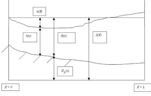
where h = h(x,t) is the height from the bed channel to the free surface, u = u(x,t) is the longitudinal velocity, g is the acceleration of gravity, c is the Chézy resistance coefficient, x is the longitudinal coordinate and t is the time. If Hb = Hb (x) is the (fixed) bottom height, measured from a constant reference plane, and if we are interested in the fluctuation η = η (x,t) from a constant free surface
S, we shall have Hb (x) + H(x) = S, where H(x) is the height from
the bottom to the constant free surface, and h(x,t) + η (x,t) = H(x); besides, amp will be the solitary wave amplitude; see Fig.
Figure 1. Longitudinal description of the channel.
We shall also take the spatial bottom variation as
H(x) = ip (1 + (x/Lc)2), (3)
where Lc is the length of the open channel and ip is the bottom
variation parameter.
The initial and boundary conditions of the problems are
η
(x, 0) = φ
1(x), 0 < x < Lc ,
u(x, 0) = φ
2 (x), 0 < x < Lc , (4)
u(0, t) = φ
3 (t) , 0 < t < T ,
η
(Lc,t) =
φ
4 (t) , 0 < t < T,
where ϕ1,ϕ2,ϕ3, and ϕ4 are convenient functions. In fact, we have assumed known the velocity at the left boundary and the fluctuation at the right boundary, but of course other combinations of boundary conditions are also possible, provided that – if the flow is subcritical – one boundary condition is given at each boundary point.
Numerical Solution of the Direct Problem:
The standard Galerkin finite element method is employed for the spatial discretization, as we show in Eq. (6) and Eq. (7). To solve this system of ordinary differential time equations it is necessary to introduce a numerical integration scheme in time; see Kawahara et
al. (1982). The scheme employed in this paper is the selective
Ms = eMl + (1-e)MG (5)
where Ms is the selective mass matrix, Ml is the lumping mass
matrix, MG is the Galerkin mass matrix and e is the lumping
coefficient. These matrices are presented in Kawahara et al. (1982) for the shallow water problem. We have considered 40 elements with a spatial step equal to 4m, and a time step of 0.05s. Kawahara
et al. (1978) created this explicit sequence in two time steps
evolutions, based on the Lax- Wendroff technique.
Spatial -Galerkin Numerical Solution:
To obtain the integration of the shallow water problem we started with the system of Eq. (1), and Eq. (2) in order to apply the Galerkin methodology but doing a splitting respect to the main operator: a linear and a nonlinear part remain; see Patil and Rao (1997). In this system H=h+η , so that
A0 d
φ
/dt = (A1 + A2)
φ
+ R(Un) (6)
With
A0 =
M 0 0 M
, A1 =
2 1 2 M M C 0
, A2 =
3 M 0 0 CI (7)
This system of ordinary differential equations represents the mass and the momentum nodal integrated equation. φ
= (η
, u) t is the vector of the unknown functions, R = (R1 ,R2 ) is the source term which includes the gradient of the bottom variation in the nonlinear part. The elements of the matrices A 1 and A2 are
M=
∫☎
NtN d✆ , C 2=-∫☎
Ntx(Nh)N d✆ ,M1=-g ∫☎
NtNx d✆ (8)
Un is the global unknown nodal vector evaluated at t
n and ✆ is the
spatial domain of integration. M2=
∫☎
Nt (Nτ ) Nu d✆ represents the
linear part of the tangential uniform stresses, N is a linear shape function in the Galerkin method and
CI=
∫☎
Nt (Nxh)Nu d✆ ,
M3=
=-∫☎
Nt(Nτ )Nu d✆ -∫☎
Nt (Nu)Nx d✆ , (9)
where M is the mass matrix system, CI takes into account the effect of variations of
η
and topography H which influences the mass equation and the momentum equations, M3 includes the resistanceand convective effects,
τ
= u /(c2H) is the friction parameter and cis the Chézy resistance coefficient.
We implemented two temporal discrete evolutions. The first one is the solution of the linear part divided in two time steps; a similar approach was taken for the nonlinear part.
First Half Time Step of the Linear Part:
ui
n +½
=(1–e)uni-1/6+(2+e)ui
n
/3+
+(1–e)uni+1/6–
✞
g(-½uni-1+½uni+1)/2-
-✞ τ (u
n
i-1/6+uin/3+uni+1/6)/2, (10)
η
in+½=(1–e)
η n
i-1/6+(2+e)
η
in/3+ +(1–e)η n
i+1/6–
✞
(auni-1+buin+d ui+1)/2, (11)
where uin+½ and
η
i n+½ are the discretized velocity and height
evaluated at tn +½ and at the spatial point xi. For each node, the
coefficients a, b and d are determined by the bottom variation.
Second Half Time Step of the Linear Solution:
In this case, the discretization according to the linear part of Eq. (6) renders the following equations:
ui
n + 1
= (1 – e)uni+1/6 + (2 + e)ui n
/3 +
+ (1 – e)un i+1/6 –
✞
g(- ½un
i-1 + ½uni+1) -
-✞ τ (u
i-1 n+½
/6 + ui
n+½
/3 + ui+1 n+½
/6) (12)
η
in+1 = (1 – e)
η n
i-1 + (2 + e)
η
in/3 +
+ (1 – e)η n
i+1 -
✞
(aui-1n+½ + buin+½ + dui+1n+½) (13)
where ✞
= ✟ t/✟ x .
First and Second Time Steps of the Nonlinear Part Evolution:
In this part of the solution we show the following explicit solution for the nonlinear operator, from tn+1 through tn+3/2 until tn+2
with a time step equal to ✟ t /2.
η
in+3/2 = (1 – e)/6
η
i-1n+1+(2 + e)/3
η
in+1+ (1 – e)/6
η
i+1n+1-
- ✞
/2 (p11η
i-1n+1+ p12
η
in+1+p22
η
i+1n+1
)-✞
/2 R1n (14)
Vin+3/2 = (1 – e)/6
η
i-1n+1+(2 + e)/3 Vin+1+
+(1 – e)/6 Vi+1n+1-
✞
/2 (p11 Vi-1n+1+ p12 Vin+1+p22 Vi+1n+1)-
- ✞
/2 (m11 Vi-1n+1+ m12 Vin+1+m22 Vi+1n+1) (15)
Vin+2 = (1 – e)/6 Vi-1n+1+(2 + e)/3 Vin+1+ (1 – e)/6 Vi+1n+1-
-✠
/2 (p11 Vi-1n+3/2+ p12 Vin+3/2+p22 Vi+1n+3/2)-
-✡
/2 (m11 Vi-1n+3/2+ m12 Vin+3/2+m22 Vi+1n+3/2) (16)
n
V is an auxiliary variable to find the discrete solution at step n+2,
i
a
is a subindex that refers to the spatial point i and nl indicates anonlinear discretization term.
η
in+2 = (1 – e)/6
η
i-1n+1+(2 + e)/3
η
in+1+ (1 – e)/6
η
i+1n+1-
- ✠
/2 (p11
η
i-1n+3/2+ p12
η
in+3/2+p22
η
i+1n+3/2)
-✡
/2 R1n
(17)
The coefficients m and p and the source terms are obtained by
numerical integration using the Gauss-Legendre method.
Sensitivity Analysis
Let us consider a functional response given by
R = <S+ , φ > (18)
where R is the response functional, S+ is the source term of the adjoint differential equation, <, > is the inner product in an adequate functional space and φ is the variable under study. The mean
values of height and velocity in the phase space are defined, respectively, by
1
m
ϕ = 1/LT ∫∫x,th(x, t) dt dx ,
2
m
ϕ = 1/LT ∫∫x,tu(x, t) dt dx (19)
As we can see in Lima et al. (1998), Eq. (1) to Eq. (2) can be
written
m = Hoφ = 0, (20)
where H0 is a nonlinear operator which applied to φ reproduces Eq.
generic parameter pi, (see Oblow (1976), Cacuci et al. (1980), Lima
and Alvim (1986), we obtain
∂
m1/pi =
∂
(h/i)/
∂
t+
∂
((u h)/i)/
∂
x
∂
m2/pi =
∂ (u/i)/ ∂ t+ ∂ (0.5 ∂
u2/
∂
x)/
∂
pi+
+g
∂
((h–H)/i)/
∂
x+((2u/c2)(u/i)/h sgn(u)–
-((u/c)2(h/i)/h2sgn(u)) (21)
( . )/i is the partial derivative of the function ( . ) respect to the
independent parameter
p
i
.Adjoint Function:
The adjoint system is given by
∂ϕ1*/∂ t=-u∂ϕ1*/∂ x-g ∂ϕ2*/∂ x–sgn(u)u2ϕ2*/(ch)2– S+ (22) ∂ϕ2*/∂ t=-h∂ϕ1*/∂ x u ∂ϕ2*/∂ x+2 sgn(u)uϕ2*/(c2h)–S+ (23) where sgn(u) indicates the sign of u, and the sources terms are
S+=1/(L
cT) (24)
where Lc is the channel length and T is the total simulation time.
The source terms of the adjoint equations (the mean heights and velocities) are the weight functions of Eq. (22) and Eq. (23), respectively. Then, the units of the the source terms depend on each analyzed adjoint functional; the correspondent units of ϕ* will be
define to make the adjoint differential equation H*ϕ*=S+
dimensionally right.
The initial and boundary conditions are given by
ϕ1*(Lc,t)=0, ϕ2*(Lc,t)=0, 0< t <T , (25)
ϕ1*(x,T)=0, ϕ2*(x,T)=0, 0<x<Lc , (26)
The conditions for the solution of the adjoint equation are chosen in order to cancel the unknown terms of the bilinear concomitant P between φ /i and φ . The bilinear concomitant is
given by
P1=∫x
T * φ h/i 0 1 dx+ ∫x T * φ u/i 0 2
dx+
+ g∫T
(
)
L * φ /i H h 0 2 − dt + ∫T
L u/i * φ h 0 1
dt, (27)
P2=∫T
T * φ h/i u 0 1 dt+ ∫T T * φ u/i u 0 2 dx ∫T L u/i * φ 0 2
dt, (28)
P=P1 + P2. (29)
We follow the procedure described in Baliño et al. (2001). For
this particular case P is given by
P=
∫
xφ*
1(x=0) ∂ h/∂ pi (t=0) dx
-∫
T ∂(h-H)/∂ pi (x=0) *φ
2(x=0) dt. (30)
X is the one-dimensional spatial domain and x=0 is the origin.
Sensitivity Coefficient:
The general sensitivity coefficient is given by
Si = < ϕϕϕϕ* , S(i) > = ϕ1* S1(i) + ϕ2* S2(i) + P (ϕ /i, ϕϕϕϕ) . where φ
*=(
φ
1*, φ
2*) is the adjoint functional vector. The first coordinate is associated to heights and the second to velocities. S1(i) and S2(i) are the source terms corresponding to Eq. (22) and Eq. (23). The sensitivity coefficients are taken with respect to the analyzed parameters, namely the Chézy resistance coefficient (c), the bottom parameter (ip) and the solitary wave amplitude coefficient (amp) which are given, respectively, by
S1 = < (φ *
1 , *
φ
2), (0,-2u 3
/c3h sign(u))>+P(φ /i,φ ) =
=
∫∫
x,t
*
φ
2 -2 u2/c3h sign(u) dx dt+P(φ /i, φ ) (31)
S2 =< ( *
φ
1 , *
φ
2 ), (0,-g)>+P(
φ /i,φ )=
=
∫∫
x,t
*
φ
2 -g 2 x/Lc2 dx dt+P(φ /i, φ ) (32)
S3= -
∫
x *
φ
1 (x=0) ∂ h/∂ pi(t=0) dx +
+
∫
T - ∂ (h-H)/ ∂ pi(x=0) *
φ
2(x=0) dt (33)
Results and discussion
Direct Computation:
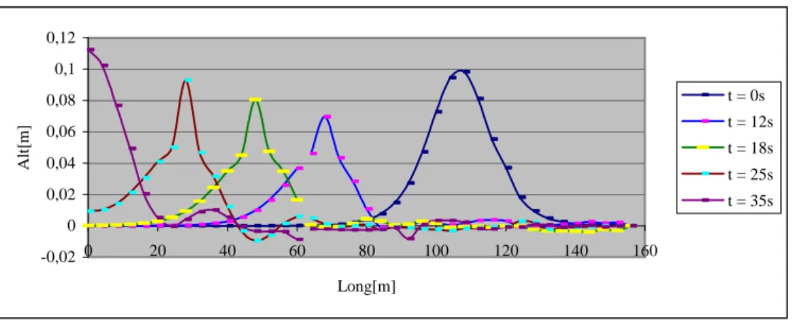
To evaluate the direct solution given in Fig. 2 we have considered the entrance of the solitary wave to a 160m long channel. This problem was solved by Zienkiewicz et al. (1993), Zienkiewicz and Ortiz (1995) and Kawahara et al. (1978, 1982). In spite of the channel length, the characteristics of the bottom resistance and the topography are very different, but the qualitative form of the solitary wave propagation results similar. Another alternative is to obtain the solution by a splitting method as in Patil and Rao (1997). We can solve the linear part by the “mass lumping” methodology which is an initial condition to the second half time step that we can solve by the same methodology, as we showed before. The friction (in the initial times) softens the solitary wave more than is shown in the results found by Kawahara et al. (1978), Kawahara and Yokoyama (1980), Kawahara et al. (1982), Zienkiewicz et al. (1993) and Zienkiewicz and Ortiz (1995). These effects are due to the large channel length, four times larger than that used by Zienkiewicz and his colleagues. These differences are also influenced by the concavity of the quadratic bottom variation. Besides this fact, we have taken, as initial velocities, a quiet lake condition different from what we found in the previous literature. As velocities are not significant we may neglect them, as we can see in the previously mentioned works by Zienkiewicz and his colleagues. We have preferred to maintain the open channel length equal to 160m at the opposite direction of the flow. The bottom variation adopted corresponds to Eq. (3). The system considered is given by Eq. (1) and Eq. (2) with all the nonlinear terms. The initial and boundary conditions are given by
η
(x,0)=a sec h2 (3½ a/2(x–1/
α )), 0<x<160m,
u(0,t)=0 , 0<t<T, u(x,0)=0 , 0<x<160m ,
η
-0,02 0 0,02 0,04 0,06 0,08 0,1 0,12
0 20 40 60 80 100 120 140 160
Long[m]
A
lt
[m
]
t = 0s
t = 12s t = 18s
t = 25s t = 35s
Figure 2. Direct solution.
Table 1 shows the physical and geometrical parameters which are being used int the direct and adjoint numerical computation.
Table 1. Physical and Geometrical parameters.
Total time simulation T=35.0s Channel length Lc=160.0m Chézy resistance coefficient c=60.0m1/2s-1 Solitary wave amplitude amp=0.1m Elemental length ∆x=4.0m
Time step ∆t=0.05 s
Coefficient of bottom variation ip=1.0 Gravity acceleration g=9.81m/s2 Stabilization factor e=0.675
Figure 3 shows the mean functional variation of the height function versus the initial amplitude of the solitary wave. We can observe small divergences between the calculated values through the direct and perturbative methodologies. We can also observe a functional increment with this parameter and an asymmetry between
these differences in both curves. To the left region with respect to the reference point (around 0.1m), these differences are more significant. This asymmetry shows a selected region near the reference point to calculate the sensitivity coefficient
0,019 0,0195 0,02 0,0205 0,021 0,0215
0,09 0,095 0,1 0,105 0,11
am [m]
Direct Perturbat ive
Figure. 3. Mean height functional corresponding to the solitary wave amplitude.
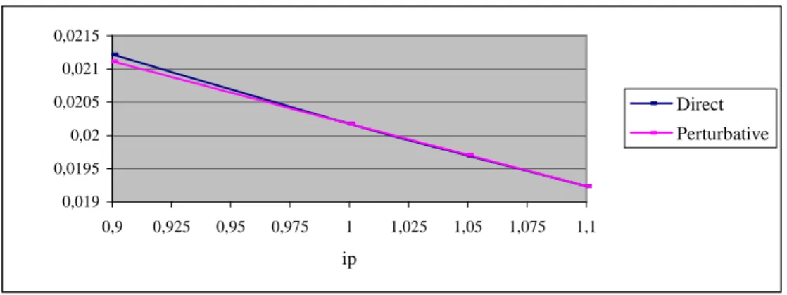
Figure 4 shows the mean height function corresponding to the quadratic bottom variation and is given by the already proposed equation H(x) = ip(1+(x/Lc)2). Both methodologies (differential and
direct) are similar and the results are coincident in ip=1. The monotonic decay characteristically happens when the flow direction is opposite to positive bottom slope. According to the calculated values and the height curvature indices of the bottom function (near
ip=1.1) it produces a minimum point that means a modified
hydrodynamics regime.
0,019 0,0195 0,02 0,0205 0,021 0,0215
0,9 0,925 0,95 0,975 1 1,025 1,05 1,075 1,1
ip
Direct Perturbative
Figure 4. Mean height functional corresponding to the quadratic bottom variation.
Table 2 shows the errors in the sensitivity coefficients corresponding to both parameters in study. As these coefficients have been calculated normalizing them so that they are dimensionless, the errors can be compared. The error in the
computation of the solitary wave amplitude sensitivity coefficient is very small; both parameters are important to be considered for sensitivity studies. The signs of the sensitivity coefficients show concordance with the physical meaning.
Table 2. Sensitivity coefficients.
Funcionales Parámetros ∆ p (φm)dir (φm)dif (CS)dir (CS)dif Errores%
amp 5% 0.020617 0.0206167 0.088000 0.087950 0.053 (φm)ref= 0.020177
ip 5% 0.019695 0.0197071 -0.009140 -0.009364 2.440
Conclusions
We applied the “mass lumping” methodology to solve the solitary wave propagation (direct method). The problems considered are: simplified model with horizontal and quadratic bottom variation and model with all nonlinear terms and linear and quadratic bottom variation. All of these cases constitute a direct validation. These results were compared with results in other papers (Zienkiewicz et
al. (1993), Zienkiewicz and Ortiz (1995), Bemansour and Wrobel
(1997), Patil and Rao (1997)) and the comparison was satisfactory. Particularly we see that the bottom and its concavity have a great influence in the open surface distribution. Also, the independence of this mean functional respect to the Chézy resistance coefficient was observed. For this reason we do not present a sensitivity analysis respect to this parameter. The methodology described in this paper for the sensitivity analysis allows us to obtain sensitivity coefficients respect to the mean height without building a response surface used in the direct methodology. So, we solve only one time the problem of the one-dimensional shallow water equation. We conclude that the mean height functional is more sensitive respect to the initial solitary wave amplitude than to the bottom parameter distribution. Also, the mean height functional is not affected by the velocity variations and, then, this problem is not good enough to study the variation of the functional respect to the resistance parameter. On the other hand, to continue studying the sensitivity of the mean height functional we prefer to choose the entrance of the tidal wave to the open channel with a quadratic bottom distribution. Finally, it is important to emphasize that the perturbation method may be applied to sensitivity studies in more complex situations. Some works (Ionescu-Bujor and Cacuci (2000a), Ionescu-Bujor and Cacuci (2000b), Cacuci (2000)) are examples of an application to a very sophisticated case. Our aim is to continue this approach to eventually apply the method to the complete shallow water equation and so to substantially improve the efficiency of model calibration,
always a difficult inverse problem in fluvial and maritime hydraulics.
Acknowledgements
The authors would like to acknowledge the Conselho Nacional de Desenvolvimento Científico e Tecnológico-CNPq (National Agency for Scientific and Technological Development) and the University of Buenos Aires (grant I050) and Fundación Antorchas for financial support.
References
Baliño, J.L., Larreteguy, A.E., Lorenzo, A.C., Padilla, A.G. and Lima, F.R.A., 2001, “The differential perturbative method applied to the sensitivity analysis for waterhammer problems in hydraulic networks”, Applied
Mathematical Modelling, Vol. 25, pp. 1117-1138.
Bemansour N. and Wrobel, L.C., 1997, “Numerical simulation of shallow water wave propagation using a Boundary Element Wave Equation Model”, International Journal for Numerical Methods in Fluids, Vol. 24, pp. 1-15.
Cacuci, D.G., Weber, C.F., Oblow, E.M. and Marable, J.H., 1980, “Sensitivity theory for general systems of nonlinear equations”, Nuclear
Science and Engineering, Vol. 75, pp. 88-110.
Cacuci, D.G., 2000, “Dimensionally adaptive dynamic switching and adjoint sensitivity analysis: new features of the RELAP5/PANBOX/COBRA code system for reactor safety transients”, Nucl. Eng. Des., Vol. 202, pp. 325-338.
Fraidenraich, A., Jacovkis P.M., and Lima, F.R.A., 2001, “Sensitivity computations using perturbative methods for the viscous Burgers equations”,
Annals of the VII International Seminar on Recent Advances in Fluid Mechanics, Physics of Fluids and Associated Complex Systems, CD-ROM,
Buenos Aires, Argentina.
Fraidenraich, A., Jacovkis, P.M., and Lima, F.R.A., 2003a, “Sensitivity Computations Using First and Second Order Perturbative Methods for the Advection-Diffusion-Reaction Model of Pollutant Transport”, Journal of the
Brazilian Society of Mechanical Sciences, Vol. 25, pp. 9-15.
Methods”, International Journal of Heat and Technology, Vol. 21, pp. 77-85.
Gandini, A., 1987, “Generalized Perturbation Theory (GPT) Methods. A Heuristic Approach”, Advances in Nuclear Science and Technology, Vol. 19, pp. 205-387.
Ionesco-Bujor, M., and Cacuci, D.G., 2000a, “Adjoint sensitivity analysis of the RELAP5/MODE3.2 two fluid thermal-hydraulic code systems: I. Theory”, Nucl. Sci. Eng., Vol. 136, pp. 59-84.
Ionesco-Bujor, M. and Cacuci, D.G., 2000b, “Adjoint sensitivity analysis of the RELAP5/MODE3.2 two fluid thermal-hydraulic code systems: II. Application”, Nucl. Sci. Eng., Vol. 136, pp. 85-121.
Kawahara, M., Takeuchi, N., and Yoshida, T., 1978, “Two step explicit finite element method for tsunami wave propagation analysis”, International
Journal of Numerical Methods in Engineering, Vol. 12, pp. 331-351.
Kawahara, M., and Yokoyama, T., 1980, “Finite Element Method for Direct Runoff Flow”, Journal of Hydraulics Engineering, Vol. 106, No, HY4, pp. 519-534.
Kawahara, M., Hirano, H. and Tsubota K., 1982, “Selective Lumping Finite Element Method for Shallow Water Flow”, International Journal for
Numerical Mehods In Fluids, Vol. 2, pp. 89-112.
Lima F.R.A. and Alvim, A.C.M., 1986, “Tempera-V2: Um Programa para Análise de Sensibilidade num Canal Refrigerante de Reatores Nucleares”, PEN-139, Programa de Engenharia Nuclear COPPE/UFRJ.
Lima, F.R.A., Gandini, A., Blanco, A., Lira, C.A.B.O., Maciel, E.S.G., Alvim, A.C.M., Silva, C.F., Melo, P.F.F., França, W.F.L., Baliño, J.L., Larreteguy A.E. and Lorenzo, A., 1998, “Recent advances in perturbative methods applied to nuclear and engineering problems”, Progress in Nuclear
Energy, Vol. 33, 1/2, pp. 23-97.
Oblow, E.M., 1975, “Sensitivity theory from a differential viewpoint”,
Nucl. Sci. Eng, Vol. 59, pp. 187-189.
Patil, M. and Rao, B.V., 1997, “Use of eigenvalue technique in finite element tidal computations”, International Journal for Numerical Methods
in Fluids, Vol. 24, pp. 953-963.
Stoker, J. J., 1957, “Water waves”, Interscience, New York, 567 pp. Zienkiewicz, O.C., Wu, J. and Peraire, J.A., 1993, “New semimplicit or explicit algorithm for shallow water equations”, Journal of Mathematical
Modelling and Science Computing, Vol. 1, pp. 31-49.
Zienkiewicz, O.C. and Ortiz, P.A., 1995, “Split-characteristic finite element model with shallow water equations”, International Journal of