Hedging options in a garch environment: testing the term structure of stochastic volatility models

lo

LOCAL:

DATA:

Fundação Getulio Vargas

E

p

_G

_E

Escola de Pós-Graduação em Economia

SEMINÁRIOS DE PESQUISA ECONÔMICA II (2

a

_parte)

~~.mJ)G:lNG O~TIONS

IN A GAaell

IJNVmONXIINT; TI18TING TBB

T~

• •

8TaVCTVI\II OI' 8TOCIIASTIC

VOLATILITT 1lI0DBLS"

j

Robert Engle

(University ofCalifornia)

Fundação Getulio Vargas

Praia de Botafogo, 190 - 14° andar Auditório

~ HORÁRIO:

12/ 12/94 (segunda-feira) 16:30h às 18:00h

\marf. .

Coordenação: Prof. Pedro Cavalcanti Ferreira

Hedging Options in a GARCH Environment:

Testing the term structure of stochastic volatility

models

Abstract Robert F. Engle Joshua Rosenberg October 1994 Department of Economics University of California, San Diego

This paper develops a methodology for testing the term structure of volatility forecasts derived from stochastic volatility models, and implements it to analyze models of S&P500 index volatility. U sing measurements of the ability of volatility models to hedge and value term structure dependent option positions, we fmd that hedging tests support the Black-Scholes delta and gamma hedges, but not the

simple vega hedge when there is no model of the term structure of volatility. With various models, it is difficult to improve on a simple gamma hedge assuming constant volatility. Ofthe volatility models, the GARCH components estimate of term structure is preferred. Valuation tests indicate that all the models contain term structure information not incorporated in market prices.

I.

lotroduction

Engle and Rosenberg

-2-Estimating the tenn structure of volatility has, in the past, focused on option implied volatility. For instance, Stein (1989) estimated the tenn structure of volatility using an autoregressive volatility model based on short tenn S&P100 option implied standard deviations. He found the actual sensitivity of medium tenn to short tenn implieds was greater than the estimated sensitivity from the tenn structure, and concluded that option markets overreact to infonnation. Diz and Finucane (1993) rejected the overreaction hypothesis using different estimation techniques.

Heynen et. alo (1994) estimated the tenn structure of volatility by comparing how well elasticity parameters generated by autoregressive volatility (AR V), GARCH, and EGARCH models explained the relationship between long tenn and short tenn implied variances for Philips and the EOE indexo The EGARCH model was found to best model this relationship, and, thus to represent the best estimate of the tenn stnlchlre ofvolatility. Xu and Taylor (1994) used regression and Kalman filter techniques to fit a tenn structure model to the time series of forward implied variances for currency options.

Since we cannot observe actual market volatility, tests ofthe perfonnance ofthe tenn structure implied by different volatility models necessarily take an indirect fonn. The previous papers use the implied volatility of different maturity options as point estimates of the tenn structure of average volatility. This paper takes a different approach. Since option prices are an observable feature, and their behavior is detennined by the underlying asset's volatility, tests based on option prices provi de another metric. We perfonn two types of tests using option prices.

•

First, volatility models are compared by their success in constructing minimum risk portfolios of medium term and short term options, and, second by their ability to obtain excess profits in options trading.

In

the first case, a medium term option (call, put or straddle) is held and hedged with other assets. The hedge is initially designed to eliminate frrst order price risk which can be undertaken by selling or buying an appropriate amount (delta) ofthe underlying stock. A more effective hedge also involves selling a second option to eliminate the second order risk associated with non-linearity of the price response (gamma) or the risk associated with a volatility shock (vega). It is assumed that this hedge should be constructed with the most similar available short term option.

The optimal munber of short term options to hold per long term option, the hedge ratio, depends on sensitivity of the options prices to volatilities and on the

estimated tenn structure ofvolatility. Ifmovements in a state variable affect primarily short volatilites rather than long volatilities, then it will take relatively few short options to hedge this risk. The term structure of volatility forecasts measures exactly this response.

In

other words, lmderstanding the term structure of expected average volatility, which generates the term structure of sensitivities, is an essential element to the hedging processo

At the end of the paper the models are used to check for mispricing of options due to the term structure. Time spreads consist of identical options with different maturities. Hence, accurate valuation requires correct estimation of the leveIs of medium and short term average expected volatility. Purchasing a time spread is a bet that short tenn volatility is underestimated and medium term volatility is overestimated by the market, while selling a time spread is a bet on the converse.

•

Engle and Rosenberg

-4-Another tenn stnlcture dependent position is a jelly roll, which consists of one call time spread held long and one put time spread held short.

This paper is stuctured as follows. In Section II option pricing is discussed and in section

In,

a methodology for hedging options in discrete time is developed, since the stochastic volatility models used are in discrete time. Section IV derives and interpretes hedging ratios for the stochastic volatility models. In Section V, the stochastic volatility models are esti.mated and their perfonnance is tested by

comparing hedging effectiveness and options trading profits. Finally in Section VI, some conclusions are drawn.

11. Pricing Options in a Stochastic Volatility Environrnent

Pricing options in a stochastic volatility envirorunent is not a solved problem, at least in practice. Theoretically, the value of a European style put option which eliminates arbitrage possibilities can be fOtmd from

(1)

~

=

E/[max(K -

Sr,O)]

where the expectation is taken with respect to the risk neutra! distribution as of time t. In the equation, K is the strike price, S is the W1derlying price and T is the expiration date and the risk free rate of interest is taken to be zero for ease of notation. This expression is on1y useful once the risk free conditional distribution is specified and this paper can be thought of as seeking useful parameterizations.

When the lmderlying asset follows a geometric Brownian motion with constant volatility, then it is well known that a solution to (1) is the Black-Scholes(1973) formula which can be written as

i

(2)

Pr

= BS(a,St,T)

where cr is the constant volatility which is also the average daily volatility over the life of the option. Hull and White (1987) point out that if volatility is independent of the stock price path, then the expectation conditional on average volatility, can be taken conditionally in (1) to get

as long as ST is conditionally lognonnal. For at-the-money options, the Black Scholes fonnula is approximately linear in volatility and therefore a striking simplification ofHull and White is the Black Scholes-Plug-in or BSP given as

(4)

Pr

= BSP(E/(a),SpT)

Various options pricing fonnulae result from various assumptions about the process of the volatility.

In each case however, it is natural to suppose that the most recent stock price St wlúch is known would have potential value in forecasting average

volatility over the life of an option. Thus the optimal forecast will be expressed as a function the stock price.

Hedging parameters are then derived by differentiating BSP with respect to the volatility model's random variables as well as the familiar variables in BS.

An approach which does not rely on the plug-in fonnulation can be implemented direct1y from (1) using simulation methods and particular specifications of the risk neutra! distribution.

Engle and Rosenberg

-7-stochastic volatility process and wiil be combinations of the BS delta, gamma and vega. For example, the stochastic volatility (SV) deita is given by

(7)

For alI the volatility processes used here, the frrst derivative ofvariance with respect to price is zero since both positive and negative price movements increase volatility. However, models such as the EGARCH and AGARCH will have non-zero first derivatives and will therefore affect the deIta's.

More interestingly, the gammas are potentially very different in a stochastic volatility enviromnent from those in a Black Scholes environrnent.

(8)

r

sv =

r

BS + A BS 1 A

J-ê?

2

20-

as

t+l St+l =St

The gamma effectively incorporates both a volatility hedge and a change in delta hedge. No longer is volatility hedging different from simply responding to the magnitude of possible changes in S. For each proposed volatility model there is a different grumna which will be labeled for the volatility processo For example, if the underlying process is assumed to be a GARCH process, then the hedge parameter will be caIled a GARCH grunma.

The optimal hedge for an option position, wiIl form a portfolio which reduces the exposure to various risk factors. Thus it forms portfolios which have zero

derivatives with respect to underlying state variables. The easiest way to fonu a delta neutral hedge is to short 1/~, of the tU1derlying asset. Since a put has a negative delta, the hedge involves a long position in the underlying asset. A

straddle will typically have a delta elose to zero already alld therefore only small

amounts ofthe underlying asset need be added to the portfolio.

To fonn a vega hedge, a second option contract is required.

As

both assets will

have vega's the optimal portfolio is short

A/ A₂

contracts of the second option.

Similarly, gamma hedge ratios will be givell by the ratio ofthe gammas,

r/r

₂. In

each case, the hedge ratio is the number of contracts of the second option which

are used to hedge the fust.

In

order to compare the effectiveness of various hedging strategies, a series of

hedged portfolios will be constructed based upon a particular theory ofhow the

hedging should be accomplished. Each position will be held for one day. The

retums on this series of portfolios will then be examined for effectiveness in

hedging risks. The simplest measure of success is simply the variance ofthe

portfolio, however measures which are illsensitive to big shocks such as the

inter-quartile range are also constructed. In addition, the portfolio returns are regressed

on the underlying retum and return squared to see whether these risk factors are

effectively eliminated. Finally the portfolio returns are checked for serial

correlation and ARCH. Any finding of serial correlation suggests a mispricing of

the assets but there is no reason to suspect these portfolios would have constant

variances so the ARCH test is merely descriptive.

IH. Stochastic Volatility Models

F our models of the volatility process are examined in this paper: the constant

volatility model (CV), the autoregressive volatility model (ARV) which infers the

tenn structure from implied volatilities, the GARCH(1, 1) model, and the GARCH

components model. Details about each of the models are in Appendix A. These

•

Engle and Rosenberg

-9-mo deIs differ in structure and in the type of fundamental shocks they allow to

drive the volatility processo

In

the CV model, no shock affects volatility, while

in

the AR V model, shocks independent of the underlying price process drive the

volatility processo

In

the .GARCH models, squared price shocks drive the volatility

processo The types of shocks that must be hedged in the option portfolio depend

on the volatility model.

Each ofthese models i.mplies a different tenn structure ofvolatility. The CV

modelleads to a flat term structure while the others generally allow it to have

either an upward or downward shape.

Begin by specifying the AR V model as this is an approximation of what

sophisticated traders use on Wall Street and has been described by Steil1(l989)

and Heynen,Kemna and Vorst(1994). Let

O'lt

be the implied volatility ofthe frrst

option contract on day t and

0'21

the i.mplied volatility of the second contract which

is being used for hedging. These can be related by a regression:

in which À could be estimated by least squares and is interpreted as the partial

derivative of the first variance with respect to the second variance. Because of the

substantial serial correlation in 11, this can perhaps be better esti.mated in

differenced fonn:

This

À.

ca11 be used to construct optimal vega hedge ratios. Since the long

volatility is estimated to move only a fractio11

À.

as much as the short, the vega

hedge ratio becomes

A1À.cr/AlJ1•

This lambda however refers only to one pair of maturities so that it is not very

useful. Because each of these volatilities is the average of the volatilities for the

remaining life of an option, it is natural to parameterize these in tenns of the one

day volatilty parameter.

where

O)

is the long run constant variance, so that

(12)

so that the lambda for contracts with maturity TI and T

2

is:

(13)

This allows time variation in the hedge ratio and sensitivity to the maturity of the

contracts. To estimate p, requires simply backing it out from (13) where a

particular À.

is estimated from the data 011 implieds. Notice that there is no

historical data 011 the underlying asset used in this procedure .

• rBUDTEC~ MARIO HENRlaUE SIMONSErt

FUNDAÇÃO GETÚLIO VARGAS

~~-'----'--=C---

--~~~----•

Engle and Rosenberg

-11-The GARCH model does use historical data from the underlying asset to estimate the process of volatility~ these parameters are then used to forecast the term structure ofvolatility. The GARCH model can be expressed as

where ~ = 10g(S/St_l), 0'2 is the one day volatility, and ú) is the long run volatility. For this model, multistep forecasts are easily computed from the oue step

conditional variances. The average variance from t tU1til TI is given by

(15) _O'it=OJ+-

')

1 [1 -

(a

+

f3)Tl](

f3

_ot"+l-OJ --.2 )

11

1-

a-This model, like the AR V model, implies a monotonic upward or downwards sloping tenn stnlcture which mean-reverts at a rate alpha plus beta.

The GARCH components model was proposed by Engle and Lee(1993) and allows more complex lag distributions. It models volatility as mean reverting to a long run component of volatility, but this long run component itself mean reverts to a constant leveI. The process for volatility can be written as:

(16)

07

=qt

+a(e;-l-qt)+~~-l-qt)

qt

=

OJ+ P(qt-l - OJ)

+

~if-l

-

~-l)

where q is the long run component which mean reverts to ú) with a rate p, while instantaneous volatility cr mean reverts to q at a rate

a+p.

This term structure is not necessarily monotonic since the day ahead, trend, and long term forecast all

•

•

influence the n-step ahead forecasts. The forecast of the average volatility from t to TI is now given by:

To compute GARCH gammas, the derivatives of (15) and (17) are simply substituted into (8). Since these derivatives are taken with respect to St+l' these fonnulaes are derived by first advancing time one day further and then recognizing that there are only T 1-1 days remaining in the contract.

To get a sense of the differences between these hedging parameters, consider first the Black Scholes hedge ratios for a standard maturity where the long option has 30 days to maturity while the option used to hedge has only 10 days to maturity. In this case the familiar vega hedge shorts 1.73 of the near contracts for each far contract. The hedge ratio exceeds one which is counterintuitive but is a reflection ofthe increase in vega with maturity. Afterall, tlús corresponds to an experiment where the volatility parameter is changed once and for alI and therefore has a bigger impact on the Ionger lived options.

In contrast, the BS gamma hedge ratio is only .57 indicating just over half a near contract be shorted for each far contract. Again, tlús is intuitive since the second derivative of the current stock price has dramatically reduced impact over longer horizons. For at-the-money options, the term structure of gamma is upward sloping indicating that nonlinear impact of a price shock is greater for short term options than longer tenn options. This implies tllat the gamma hedge ratio is less than one, wlúch is consistent with intuitioll. In contrast, away-from-the-money, the tenn struchlre of gamma is downward sloping, since elose to maturity

in-the-..

Engle and Rosenberg

-13-money options behave like the llilderlying asset, and out-of-the -13-money options are

insensitive to underlying price moves. Thus, the out-of-the-money hedge ratio will

be greater than one. See charts 3 and 4.

The hedge parameters from the stochastic volatility models are linear

combinatiolls of these two BS parameters. The AR V model operates through

vega so that the mean reversion in volatility counteracts the rise in vega. For this

standard case and the estimated model, the hedge ratio is .99 requiring a

one-for-one hedge strategy.

The GARCH gamma using these maturities, estimated parameters and typical

values is .90 while the GARCH componel1ts model is .78. Since these are linear

combinatiolls of the BS gamma and vega, they willlie between these extremes.

The shape of the tenn structure and the persistence of shocks determines how

these are weighted. In general, if only near variances are sensitive to volatility

shocks, thell the weights will give more emphasis to the BS gamma.

If

the

process is IGARCH, then more weight wiU be given to BS vega.

v.

Results

We compare the implied tenn structures of the four volatility models by

constructing hedges for near-the-money medium tenn calls, puts, and straddles

using short tenn calls, puts, and straddles. The best model should construct the

lowest risk portfolios. In addition, we compare the tenn structures by measuring

their profits in trading time spreads and jelly ro11s.

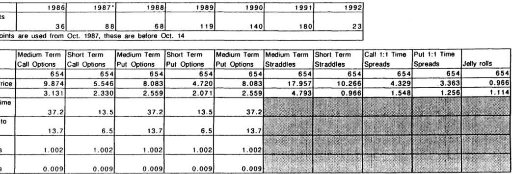
This paper uses daily data for the nearest-to-the-money Standard and Poor's 500

Index put al1d call option with closest and next-closest maturities from October

i

1985 through February 1992. The data was gathered by Chicago Board Options

Exchange. Only the 654 data points for which option prices are available for the

medium and short tenn calls and puts are inc1uded in the analysis. Options that are

further than five percent from the money are exc1uded. See Table 1 for details.

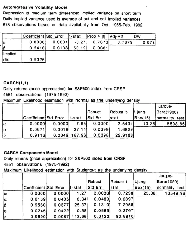
Estimating the Volatility Models

The first step in the testing procedure was estimation of the stochastic volatility

models. See Table 2 for details. The ARV model was estimated using an OLS

regression of differenced implied medium tenn variance on the differenced

implied short tenn variance. The beta from

this regression, .54 ,implies a rho of

.93, assuming that the long tenn option has 37 days to maturity and the short term

option 13. Diz and Finucane use Maximum Likelihood Estimation to arrive at beta

parameters ranging from .43 to .55 for S&P100 implieds. The rho implied by these

betas range from .92 to .94.

From the implieds, there is strong evidence for mean reversion in volatility. The

change in medium tenn implied volatility is a fraction of the change in the short

tenn implied. Also, short tenn implied variances and their first differences are

more volatile than for medium tenn. That is, the volatility of volatility is dec1ining

with mahlrity. This is consistent with raw data for option prices which indicates

that short tenn option portfolios are substantially more volatile than medium tenn

portfolios.

The GARCH( 1,1) and GARCH components models are estimated using maximum

likelihood estimatioll. The GARCH(l,l) model assumes ooderlying nonnal

density, and the components model assumes that the ooderlying density is

i

Engle and Rosenberg

-15-volatility and a deelining -15-volatility of -15-volatility. The components model also exhibits this pattern. The CV model uses the one step allead GARCH(l, 1) forecast as the estimate of 'constant' volatility.

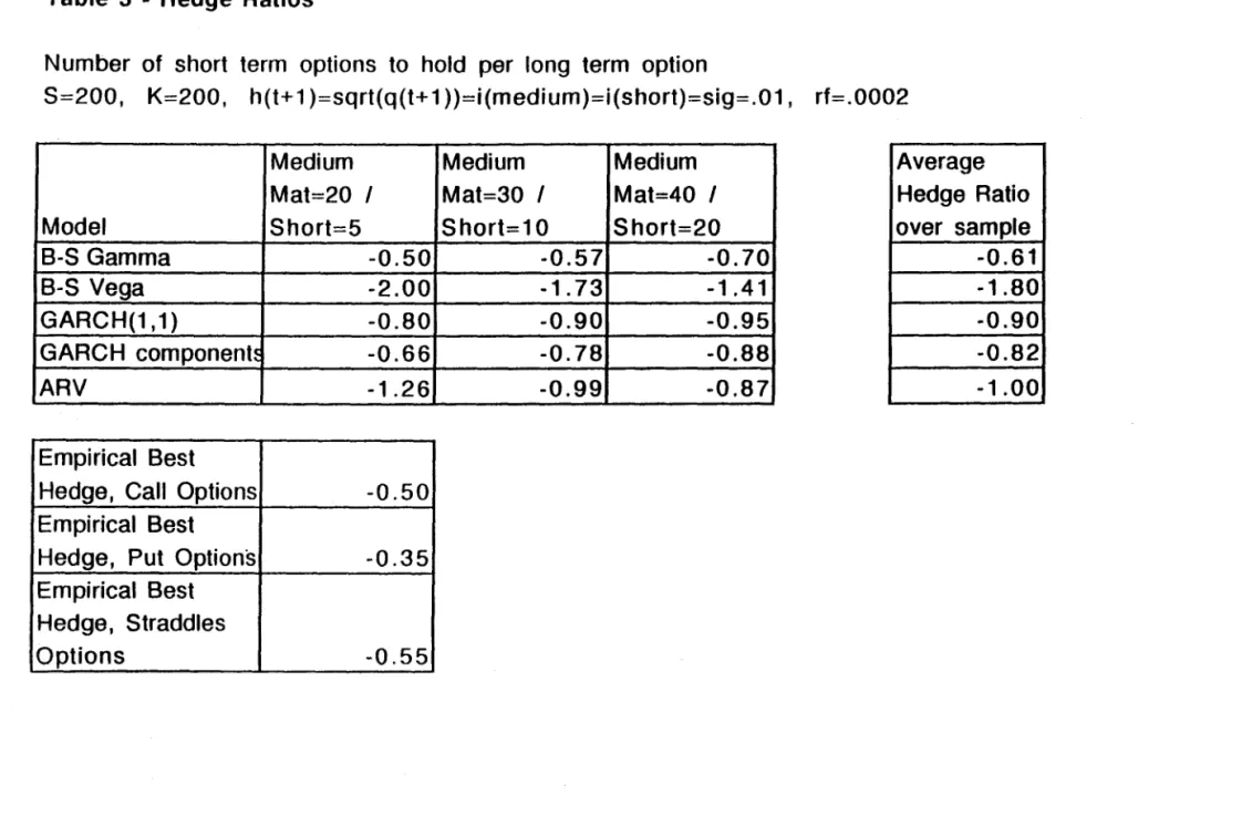
Using these models, it is straightforward to estimate hedge ratios. For an at-the-money call position, alI hedge ratios are less than one except for the CV and AR V vega hedges. This is due to the strong upward slope ofthe vega tenn structure.

In

addition, the slope of the tenn structure of hedge ratios flattens for alI models except the CV and ARV. The CV gatmna hedge atld the GARCH components hedge have the lowest hedge parameters and are also elosest to the empirical best hedge parameters. Details are in Table 3.

Hedging tests

The fust test of the tenn structure implied by the volatility mo deIs is the hedging test. It is implemented as follows. Each trading day, three one hundred dolIar portfolios are purchased. One contains medium tenn calIs, one medium tenn puts, and one medium tenn 1: 1 straddles. Then, hedge ratios are ca1culated based on the appropriate fonnula from each stochastic volatility mode!.

In

each portfolio, delta shares of the underlying are sold short, generating a zero exposure to frrst order price shocks.

For the AR V model, each portfolio is vega hedged by selling the appropriate number of short tenn options. For the GARCH(l,l) atld components model, each portfolio is gatmna hedged by selling short tenn options. The short contract is designed to match the long contract so that when long calls are being hedged, a short call is sold with the same strike. The same is true for puts and straddles. FinalIy, the entire portfolio is delta hedged with the composite delta. Two

•

Engle and Rosenberg

-17-The second best model, the GARCH components model, reduced risk over the

delta hedge by 1-10%. Its success may be due its flexible parameterization of the

tenn strllctllre of volatility, which generates faster time decay, and lower hedge

ratios.

The GARCH( 1,1) model was unable to improve on the delta hedge for calls, and

reduced risk by 2-50/0 for puts and straddles. The portfolios with hedge ratios

greater than one on average, the CV and AR V vega hedge, are the poorest

perfonners. They are unable to improve on the delta hedge for any option position.

A perfectly hedged portfolio would have no structure in its price changes. None of

the hedge pOltfolios are able to attain this goal. However, the price changes for

hedge portfolios constructed using the CV gamma and GARCH components

models are uncorrelated with the index price change and square. No model

consistently generates hedge price changes free of autocorrelation and

heteroscedasticity.

Interpretation of the Results

It

is rather surprising that the best hedge is the BS grunma hedge. Essentially this

says that the best assumption about volatility is that it is constant. This is c1early

totally inconsistent with the movements in both implied and historical volatilities.

Is it possible that we have simply considered the wrong stochastic volatility

models? While this is of course true, it will not resolve the paradoxo Any

stochastic volatility process will add some vega to the Black Scholes gamma and

wiIl generally give too large a hedge ratio. Only if movements in short term

l

voIatiIity are systematicalIy reversed afier the short term option expires can the

hedge ratio be reduced; this seems highly impIausibIe as a continuing processo

Another potential explanation for this pl1zz1e is that the Black Scholes Plug-in

approach to option pricing is systematically incorrect and produces too large

hedge ratios. To examine this possibility, we revert to the basic option pricing

model in equation (1) and simulate the risk neutral terminal distribution under

several assumptions.

In particular, this distribution is simulated under the

GARCH(l,l) and component GARCH processes estimated in this paper.

In each

case, the standardized shocks are drawn from a student-t distribution with 6

degrees of freedom to represent the leptokurtosis in the standardized residuaIs

from any volatility mode!. These are simulated for 40 days with 10,000

replications andoption prices are calculated as the expected payoff from this risk

neutral distribl1tion. The simulation is then restarted with the same random

numbers and St+! increased and decreased by .5%. Then the three option prices

alI with the same strike and maturity are used to estimate the second derivative.

This is a numerical approach to correctly calculating the GARCH gamma without

using the BIack SchoIes formula at alI.

The results are rather surprising. The simulated values are very close to the BSP

values and much higher than the BS garrunas. Even the GARCH compollellt

model with leverage which is simulated with just the same persistence as the

component model, has on1y slightly lower hedge ratio. There is no c1ear defmition

of the BSP for this case, as the function is non-differentiable.

Engle and Rosenberg

-19-HEDGE RATIOS 30days/lOdays

Model Simulated

GARCH .83

GARCH component .78

GARCH component with leverage .77

BSP BS

.90 .57

.78 .57

It appears that the problem with the hedge ratios is not a problem with the option pricing formulation, at least for these at-the-money options.

The remaining solution is that the options are mispriced. We consider the

possibility that the market misprices these options although it is also possible that the CBOE who collected the data, did the mispricing.

In

either case, the

theoretical and empirical hedge ratios could be different.

In

fact, using a portion ofthe same data set, Noh, Engle and Kane(1994) fOWld substantial evidence that GARCH models could profitably suggest when to be short or long at-the-money straddles. Furthermore, Stein(1989) claims to have found that options prices overreact to news. A systematic overreaction of short maturity options would make them excessively variable and would make a low hedge ratio optimal. This possibility is explored in the next section.

Option Pricing tests

If the options market is not efficient in that it does not incorporate alI available information into current prices, then it may be possible to earn excess profits by trading options. The options pricing tests we implement focus on whether there are better volatility forecasts than those impounded iuto market prices. We design a trading strategy that uses volatility forecasts from each stochastic volatility

model to price term structure dependent option positions. By calculating excess profits from each strategy, we can compare the accuracy ofthe model forecasts compared to the market forecasts.

The trading strategy we use is to calculate the market price of one option position. We then estimate the price ofthis position using the Black-Scholes fonnula, evaluated at forecast average volatility using a stochastic volatility mo de!. The difference between the model price and the market price is the trading signal.

The trading decision is binary: onIy one position is purchased or sold, no matter what the magnitude of the trading signal is. If the model price is greater than the market price, we asswne that the market has underpriced the option position, and purchase the position. Ifthe model price is less than the market price,we assume the market has overpriced the position, and we se11 it. At the end of each day, the position is established, and it is sold at the end ofthe following day. Ifthe market prices the next day move in the direction of the mo dei prices, the model earns a profit. Otherwise, it loses money. If the mo dei volatility forecasts are superior to the market forecasts, then the model prices are more accurate than the market prices, and the trading strategy should earn excess profit over time. The methodology is similar to that ofNoh, Engle, and Kane (1993).

In order to test the forecasts of the term structure implied by the models, we select three term structure sensitive positions for our analysis. These are aI: 1 call time spreads, aI: 1 put time spread, and a jelly ro11. The time spreads consist of a mediwn term at-the-money option held long and a short term at-the-money option held short. The jelly roll consists of aI: 1 call time spread held long and aI: 1 put time spread held short. As a comparison to Noh et. al., we also test two volatility

ItlltDTEC4 MARrO HENRIQUE SIMONS.M

FUNDACÃO GETOLlO VARGAS

Engle and Rosenberg

-21-sensitive positions: short term money straddles and medium term

at-the-money straddles.

The fOUI volatility models compared in the tests are the GARCH(l, 1) model, the

ARCH components model, the CV model, and implicitly, the AR V model. For the

constant volatility model, we

as~wne

that the best forecast of future constant

volatility i5 given by the one step ahead forecast from a GARCH(l, 1) model. This

would be more appropriate if the model estimated were an 1GARCH model,

which actually has a fiat term structure ofvolatility, like the CV model.

The AR V model is not explicitly tested, since it implies that the prices derived

from implied volatility are the correct prices. Of course, this will result in no

trades, since model prices wiIl be equal to market prices by definition. The AR V

model is taken to imply a strategy of always buying one position. Of course, it is

just as sensible to consider it as an always sell strategy, or probably even more

reasonable is to use forecasts derived from an implied volatility regression as in

Day and Lewis (1988).

The first part of Table 5 shows the average profits and standard deviation of

profits for each of the four models. 1t is noteworthy that the 'Always buy' position

earns trading profits that are not statistically different from zero at the .01 percent

leveI for the term structure sensitive portfolios, but the trading profits are

significantly negative for the volatility sensitive portfolios. This indicates that

consistent1y selling straddles was profitable over the period, implying that the

market volatility forecasts were toa high on average, while the market term

structure ofvolatilities was not biased in this way.

Engle and Rosenberg

-22-The GARCH models and CV model eam excess profits for all the term structure

sensitive positions, while the AR V model, which uses the market forecasts eams

zero profits. This indicates that there is an inefficency in the market's processing

ofvolatility infonnation to forecast the term structure. For the call time spreads,

the models eam an average profit of about 15 cents per position with a standard

deviation of about 1 doUar.The profits are slightly higher and the volatility of price

changes is lower for the put time spreads. The average prices ofthe call time

spreads are about $4.30 compared to $3.40 for the puts.

AlI of the models are predominantly option sellers as shown on the Summary of

Trading Signals. Each of the models, other than the AR V model, chooses to seU

positions at least 80% ofthe time. This indicates that overall, the models find time

spreads, jelly rolls, and straddles to be overpriced.

In

fact, alI of the models,

except the AR V model, are able to eam profits significantly greater than zero.

These tests indicate that the GARCH mo deIs are superior in pricing volatility

sensitive portfolios, and that all of the models are able to generate excess profits

for term structure dependent positions. However, the tests are not conc1usive

about the superiority of any model in estimating the term structure of volatility.

v.

Conclusions

This paper provides a methodology for testing the term structure of volatility

implied by stochastic volatility models, and implements it to analyze the term

structure of S&P500 index volatility. Hedging tests select the Constant Volatility

model using a gamma hedge, followed by the GARCH components model as best

at forecasting the term structure.

It

is argl.1ed that the surprising success of the

constant volatility model is likely to be a result of option mispricing. The

Engle and Rosenberg

-23-valuation tests concur, indicating the superiority of the GARCH models in pricing

volatility sensitive portfolios, a1though all the models excel in pricing term

APPENDIXA

Stochastic volatility mo deI

ARV: 07+1 -

&

=

Áo7 -

02]+

êr

GARCH (1, 1): df+l =

0/..) -

a-13) + ae; + f3df

GARCHcomp: df+l = qr+l + a(e; - qt) +

P

df - qt)

qt+l

=

0/...) -

p) + fXlt + r/f....e; -

07)

n - step ahead volatility

ARV: o7+klr

=

02

+

1-

1

[07 -

&]

GARCH(1,I):df+klr = co+(a+f3)k-l[o7+l - CO]

GARCHcomp: df+klr = co+ (a+ f3)k-1e df+l - qr+l) +

1-

1eqr+l - CO)

A verage volatility over T periods for GARCH, St+l = Sr

ARV: õ?"+I(T) =

&

+![I-

rI](o7+1 -

if)

T I-p

1 [I-ea+f3)T-l]

GARCH(I,I): õ?"+2(T -1) = c o + - f3) (df+2 - co)

T-I

I-(a+

_

1 {[I-

C a+ f3)T-l]

[1-

pT]

}

GARCHcomp:õ?"+2(T-I)=co+-- f3) (o7+2-qr+2)+ - - (qr+2- CO)

T-I l-(a+ l-p

Sensitivity of average standard deviation to a shock

ARV: dãt+1(T)

= _

1 [l-ri]

dêr 2o;+I(T)T 1-p

GARCH:dãt+2~T-l)=

_ 1

[1-(a+f3)T-l]d2~+2

dSr+1 2o;+2(T -1) 1-(a+ f3) dSr+1

GARCHcomp:dãt+2~T-l)

= _ 1

{[1-(a+f3)T-l]d2~+2 +[1-rl]d2q~+2}

dSr+1 2o;+2(T -1) 1-(a+ f3) _dSr+1 1-p dS_t+₁

Engle and Rosenberg

·25-Elasticity of mediurn tenn average standard deviation with respect to short tenn average stanclard deviation

ARV:Â= Ts [I-lm]O't+l(fs) Tm

l-I'

O't+l(Tm)

GARCH (1, I):Â

=

ls -I [1-(a+

,B)~m-ll]

Gt+2(ls -1)

T,n

-1 1-(a +,B) ,- _O't+2(Tm -1)

{[I-

(a+ ,B)Tm-l]d2

cr

t+1

+[1-

_{pTm-l]d 2qt+}1}

GARCHcomp:Â= ls Gt+2(ls-l) 1-(a+,B) dSt2+1 _I-p

dSt~1

Tm 0{+2(Tm-l)

{[I-(a+,B)Ts-l]d2~t+l +[I_pTs-l]d2q~+I}

Hedge Ratios CV:Gamma: rm(O') rs( 0') CV:Vega: Am(O') As(O') A (- (T.» dõ"t+l(Tm) m 0(+1 m de ARV.- t . A (O'. (T» dO(+l(ls) s t+l s de t 1-(a+,B) _dSt+1 1-P _dSt+1 GARCH (1,1): _ d20{+2(ls -1)

rse

O't+2(Ts

-I»

+ As(O't+2(Ts

-I»

2

dSt+1

Bibliography

Black, Fischer and Myron Scholes, 1973, The Pricing ofOptions and Corporate Liabilities, Joumal ofPolitical Economy, 81, 637-654.

Diz, F. and T. 1. Finucane, 1993, Do the Options Markets Really Overreact?,

JOlilllal OfFutures Markets, 13, 299-312.

Engle, R. F. and Gary G.l Lee (1992), "A Pennanent and Transitory Component

Mode1 of Stock Retum Volatility," Discussion Paper, UC-San Diego 92-44. Heynen, R., A. Kemna and T. Vorst, 1994, Analysis Ofthe Tenn Structure Of

Imp1ied Volatilities, Joumal OfFinancial and Quantitative Analysis, 29, 31-56.

Hull, Jo1m and Alan White, 1987, The PriCillg ofOptiollS on Assets with Stochastic Volatilities, Joumal ofFinance, XLII, 281-30l.

Noh, Jaesun, Robert F. Engle and Alex Kalle, Forthcoming, A Test ofEfficiency for the S&P500 Index Options Market Using Variance Forecasts, Joumal of Derivatives, .

Stein, J., 1989, Overreactions In the Options Market, Journal OfFinance, 44,

1011-1023.

Xu, X. alld S. 1. Taylor, 1994, The Tenn Stnlcture OfVolatility Implied By

Foreign Exchange Options, Joumal OfFillancial and Quantitative Analysis, 29,57-74.

"

Table 1 . Data Summary

Table 1 - Summary 01 Options Data

Dala galhered by lhe Chicago Board Oplions Exchange, Daily, Ocr. 1987·Feb. 1992

Nearest-Io-the·money oplions for which currenl and nexl day's price are available are used in lhe Sludy

Year 1986 198r 1988 1989 1990 1991

Data Poinls

Available 36 88 68 119 140 180

'Only 5 points are used frgl'Tl Oct 1~8~hese are _ belore Ocl. 14

-Medium Term 13.5 37.2 13.5 Matur. 13.7 6.5 13.7 6.5 Average Moneyness 1.002 1.002 1.002 1.002 Sld. ness 0.009 0.009 0.009 O. 1992 23

Cal! 1:1 Time IPut 1:1 Time

Table 2 - Estimation of Stochastic Volatility Models

Autoregressive Volatility Model

Regression of medium term differenced implied variance on short term Daily implied variance used is average of put and call implied variances 678 observations based on data availability trom Oct. 1985-Feb. 1992

Coefficient Std Errar t-stat Prob > Itl Adj-R2

j.! 0.0000 0.0001 -0.27 0.7873 0.7879

~ 0.5418 0.0108 50.19 0.0001

Implied

rho 0.9325

GARCH(1,1)

Daily returns (price appreciation) for S&P500 index from CRSP 4551 observations (1975-1992)

DW

2.672

Maximum Likelihood estimation with Normal as the underlying density

Robust Robust t-Coefficient Std Errar t-stat Std Err stat

w 0.0000 0.0000 7.95 0.0000 2.6404

a 0.0671 0.0018 37.14 0.0399 1.6829

~ 0.9116 0.0049 187.96 0.0398 22.9188

GARCH Components Model

Daily returns (price appreciation) for S&P500 index from CRSP 4551 observations (1975-1992)

Ljung-Box(15)

10.26

Maximum Likelihood estimation with Students-t as the underlying density

Robust Robust t- Ljung-Coefficient Std Errar t-stat Std Err stat Box(15)

w 0.0000 0.0000 1.27 0.0000 0.7238 25.08 a 0.0139 0.0405 0.34 0.0480 0.2897 ~ 0.9560 0.0377 25.37 0.1310 7.2958 <I> 0.0245 0.0422 0.58 0.0885 0.2767 p 0.9890 0.0087 113.96 0.0122 80.9810 Jarque-Bera(1980) normality test 5808.86 Jarque-Bera(1980) normality test 13549.96

Table 3 - Hedge Ratios

Table 3 - Hedge Ratios

Number of short term options to hold per long term option

S=200, K=200, h(t+1 )=sqrt(q(t+1 ))=i(medium)=i(short)=sig=.01, rf=.0002 Model S-S Gamma S-S Vega GARCH(1,1) GARCH component~ ARV Empirical Sest

Hedge, Cal! Options Empirical Sest

Hedge, Put Options Empirical Sest Hedge, Straddles Options Medium Mat=20 I Short=5 -0.50 -2.00 -0.80 -0.66 -1.26 -0.50 -0.35 -0.55 ~

Medium Medium Average

Mat=30 I Mat=40 I Hedge Ratio

Short=10 Short=20 over sample

-0.57 -0.701 -0.61

-1.73 -1.41 -1.80

-0.90 -0.95 -0.90

-0.78 -0.88 -0.82

Buy 100$ portfoliO of medium term positions. Delta and gamma or vega hedge. Rebalance daily.

Data: CBOE S&P500 Index Options (Oct. 1, 1985 - Feb. 28, 1992) Ljung-Box and ARCH tests are on first six lags of portfolio return

Regression is portfolio price change on contemporaneous S&P500 Index change and square Delta hedge uses GARCH(1,1) volatility forecast

Hedging Medium Term Calls

•

• Standard Raw Raw

Average Deviation of Data Data

Dai/y Dai/y Ljung- Eng/e Regres

Portfolio Portfolio Box ARCH sion F

Price Price probo

«

probo

«

probo

Position Change Changes . 01) . 01)

«

.01)

100$ Medium Term Calls 0.69 18.23 • 100$ Medium Term Calls Delta Hedged -0.43 9.27 * * 100$ S&P500 Index 0.04 0.96 * Black-Scholes Gamma Hedge -0.12 8.93 * * Black-Scholes Vega Hedge 0.79 13.28

·

• • GARCH(1,1) Gamma Hedge 0.07 9.39

·

• • Garch Components Gamma Hedge 0.01 9.24 • • Autoregressive Volatility Vega Hedge 0.26 9.87

·

•

·

Best Constant ex-post hedge 0.06 8.88 • *

Hedging medium term puts

,

Standard

,

Deviation of Raw Raw

Average Unexpected Data Data

Dai/y Dai/y Ljung- Engle Regres

Portfolio Portfolio Box ARCH sion F

Price Price probo

«

probo

«

probo

Hedge Change Changes .01) .01 )

«

.01)

100$ Medium Term Puts -1.40 20:66 • 1.00$ Medium Term Puts Delta Hedged -0.33 9.59 • 100$ S&P500 Index 0.04 0.96

·

Black-Scholes Gamma Hedge -0.08 8.54

.

* Black-Scholes Vega Hedge 0.58 16.69 * * GARCH(1,1) Gamma Hedge 0.09 9.35

.

* * Garch Components Gamma Hedge 0.05 9.06 * * Autoregressive Volatility Vega Hedge 0.26 10.87 * * * Best Constant ex-post hedge -0.38 8.88 *

Average Unexpected Data Data

Dai/y Dai/y Ljung- Engle Regres

Portfolio Portfolio Box ARCH sion F

Price Price probo

«

probo

«

probo

Hedge Change Changes . 01) .01)

«

.01)

100$ Medium Term Straddles -0.69 6.86 * 1'Ü0$ Medium T erm Straddles !)elta Hedged -0.59 6.85 * 100$ S&P500 Index 0.04 0.96 * Black-Scholes Gamma Hedge -0.25 6.02 • Black-Scholes Vega Hedge 0.64 11.38 * * GARCH(1,1) Gamma Hedge -0.05 6.49 * * * Components Gamma Hedge -0.11 6.30 * Autoregressive Volatility Vega Hedge 0.19 7.51

·

* * Best Constant ex-post hedge -0.27 6.01

·

* I

J

T able 5 - Option Trading Results

Value portlolio 01 1: 1 lime spreads (calls. puls). jelly roll. medi um and shorl term slraddle. Sell il markel price is greater Ihan model price. olherwise buy. Rebalance daily .

• Average nol dilferent Irom zero ai .01 levei

Model Always Buy - ARV model CV Model GARCH(1,1) avg

Standard Standard Standard

Average Devía/íon of Average Devíatíon Average Deviatíon of

Daífy Dai/y Dai/y of Daily Dai/y Dai/y

Portfollo Porlfofío Portfofío Porlfo/io Porlfofío Port/olio

Príce Príce Price Price Price Price

Posilion Change Changes Change Changes Change Changes

1 posilion 1:1 Call

Time Spread • -O. 008 0.99 0.16 0.98 0.16 0.98 1 posilion 1: 1 Pul Time Spread '-0.006 0.82 0.14 0.81 0.18 0.81 1 posilion Jelly RolI • -0.003 1.39 0.44 1.32 0.46 1.31 100$ Medium Term Straddle -0.69 6.86 0.89 6.83 0.80 6.84 100$ Shorl Term Slraddle -1.48 11.52 1.37 11.53 1.58 11.50

Summary oI Tradlng SIgnal9

Gareh ComponenlS Standard Average Devíation of Dai/y Dai/y I Portfolío Portfolío I Price Change Price Chanaes

0.14 0.98

0.18 0.80

0.46 1. 31

0.85 6.84

1.53 11.51

Number of Buy signals Average Profil on Buy/Sell dlfferent from O at .01 levei

GARCH(I,I) Gareh GARCH(I,l) Garch

Position ARV model CV Model avg vol Componenls Posítlon ARV Model CV Model avg vol Components

1 position 1 position

1:1 Call 1:1 Cal! Time O 10 .+/+ .+/+ · + I +

Time Spread 654 53 45 40 Spread

1 posilion 1 position

1: 1 Pul 1:1 Put Time O 10 · + I + · + I + · + I +

Time Spread 654 124 145 1261 Spread 1 posilion Jelly RolI 654 134 156 157 1 position 0/0 · + / + · + I + · + / + Jel!y RolI 100$ Medium 100S - I O · O I + · O I + .0/+

Term Medium Term

Straddle 654 49 30 20 Straddle 100$ Short 100S Short Term' ... ;

..

- ... ~ . . A n-, Ar. A A Tarm - I O · O I + · O I + · O I + 000 «::lr..,,.,.I .. • .jt ...j

~~

Term Structure of Vega

(S=100, K=100, sig=.01, rf=.0002) 400-350 3GO 250 co 0'1 200 CD > 150 100

/]M>~j

/ ./. -' ----lI 1-,_ 1'-/ v~f\' //

.f'-;1.--;//.

I( / ~ _,F J, 5 O I ~ ___ / ___ ) /' // / !--- I; .. -'. ---'- ---.~ .. J.- . / / , l ' ~ / j O 1 - - I

~r---r-~~

120115110105100 95 90 Stock Price lO .jI

\

~

\~y~~

80

'~/ ~~(

---:-y

60

&.

--~~-:.

_______ -

~~/ 4 O ---/ _{/___}

-

_{- 20} 85

- - f

5 80 75 Time to Mal. ~

.

\ ~

cu E E cu C) 0.1

a

0.16 0.14 0.12 0.1 0.08 0.06 0.04 0.02 I /

Figure 2- Gamma T erm Structure

Term Structure of Gamma

(S=100, K=100, sig=.01, rf=.0002) / --. ---~.-. ----/ 01< - ""{_" " ( 120 115 110 Stock Prlce 80 75

..

~ ~ 40 Days to Mal. 20 . , f I ., J

MAIiJI3 HENRICUE SIMONSEN

.. ~

N,Cham. P/EPGE SPE E86h

•

Autor: Engle, R. F. (Robert F.).

Título: Hedging options in a garch environment: testing

083706 1111111111111111111111111111111111111111 48154 IFGV -BMHS _{N° Pat.:Fl086/98} : 000083706 111111111111111111/11111111/111111111 e·· .e ' __ ... __ ~. ;.. .. _ _ .... -...