Information About Future Inflation?
José Valentim Machado Vicente
†
, Osmani Teixeira de Carvalho
Guillen
‡
Contents: 1. Introduction; 2. Model; 3. Data and Stylized Facts; 4. Empirical Results; 5. Conclusion.
Keywords: Inflation-Linked Bonds, Real and Nominal Yields, Term Premia, Break-Even Inflation.
JEL Code: E31, E43, G12.
There is a widespread belief that inflation-linked bonds are a di-rect source of information about inflation expectations. In this paper we address this issue by analyzing the relationship between break-even inflation (the difference between nominal and real yields) and future in-flation. The dataset is extracted from Brazilian Treasury bonds covering the period from April 2005 to April 2011. We find that break-even infla-tion is an unbiased forecast only of the 3-month and 6-month ahead in-flation. For medium horizons (12 and 18 months), break-even inflation has weak explanatory power of future inflation. Over long horizons (24 and 30 months), we report a significant, but counterintuitive, negative relationship between the break-even and realized inflation rates.
Há uma crença generalizada de que títulos indexados a inflação são uma fonte de informação sobre a inflação futura. Neste artigo, nós estu-damos essa questão analisando a relação entre a break-even inflation (difer-ença entre as taxas nominai e reais) e a inflação futura. A base de dados é extraída de títulos do tesouro brasileiro cobrindo o período de Abril de 2005 até Julho de 2010. Nós mostramos que a break-even inflation é um estimador não viesado da inflação somente para os horizontes de 3 e 6 meses. Para os horizontes médios (12 e 18 meses), a break-even inflation tem fraco poder explanatório da inflação futura. Para horizontes longos (24 e 30 meses), nós reportamos uma relação significante, porém negativa entre a a break-even inflation e a inflação realizada.
∗The first author thanks CNPq-Brazil for financial support. The views expressed in this paper are those of the authors and do not necessarily reflect those of the Central Bank of Brazil.
†Banco Central do Brasil and Ibmec. E-mail:[email protected]
1. INTRODUCTION
Market participants and policymakers interpret break-even inflation (the spread between nominal and real yields) as the main indicator of expected inflation. According to the current Federal Reserve chairman, inflation-linked bonds appear to be the most important source of future inflation expecta-tions (Bernanke, 2004). However, it is well known that the break-even inflation rate (BEIR) can be de-composed as an inflation expectation plus a risk premium term. This leads to the following questions: Does the BEIR efficiently predict future inflation? In other words, is the inflation risk premium negli-gible? A more general formulation of these issues can be stated as: Do inflation-linked bonds contain information about future prices? In this paper we shed light on these questions through a model-free procedure using data on Brazilian Treasury yields.
Our analysis is based on a series of regressions between the realized inflation (dependent variable) and the BEIR (independent variable) for the horizons of 3, 6, 12, 18, 24 and 30 months. The significance of the parameters andR2
provide a way to test the predictive ability and explanatory power of the BEIR. To avoid specification problems such as autocorrelations and endogeneity, we run these regres-sions using different approaches. First, we consider an OLS procedure. Next, we employ instrumental variables, estimating the model by TSLS and GMM techniques, with the covariance matrix computed ac-cording to Newey e West (1987).1The use of instrumental variables aims to keep consistency when the
regressor is correlated with the error term, while the Newey-West method overcomes autocorrelation in the residuals.
Many other studies have investigated the inflation risk premium and consequently the relationship between break-even and realized inflations using real and nominal interest rates. Among others, we can cite D’Amico et alii (2008), Hördahl (2008), García e Werner (2010), Joyce et alii (2010), and Grishchenko e Huang (2010). The first four papers work in an affine arbitrage-free framework. D’Amico et alii (2008) show that although the U.S. inflation-linked bond yields contain a liquidity premium and time-varying inflation risk premium, the Treasury Inflation-Protected Security (TIPS) rates are a useful proxy for inflation expectations. García e Werner (2010) apply a model similar to that used by D’Amico et alii (2008) in the euro area. They find that the term structure of inflation risk premia is upward sloping and varies from 7 to 25 basis points. Hördahl (2008) uses a structural macroeconomic model to estimate inflation risk premia in the United States and the euro area. He shows that inflation risk premia have an increasing pattern with respect to maturity for the euro area and a flatter one for the United States. Joyce et alii (2010) estimate a joint model of UK nominal and real term structures. They find that the Bank of England’s independence to set interest rates in May 1997 decreased the inflation risk premium and the inflation expectation embodied in the term structure. The article of Grishchenko e Huang (2010) computes the inflation risk premium as the difference between the TIPS break-even inflation and an estimation of future inflation. They show that the inflation risk premium is time-varying with negative values from 2000 to 2004 and positive from 2004 to 2008.
However, none of the above studies use the methodology proposed in this work. Our procedure to assess the information content in the BEIR has previously been applied in other contexts. For example, Campbell e Shiller (1991) test whether the slope of the term structure predicts changes in interest rates. To this end, they run regressions of future yields on forward yields. Christensen e Prabhala (1998) regress the realized volatility on the implied volatility of the S&P 500 to evaluate the relationship between these two volatilities. Our strategy is close in spirit to that of Campbell e Shiller (1991) and Christensen e Prabhala (1998), except we replace yields and volatility by inflation. That is an innovation of this paper: a model-free approach to measure the explanatory power of the BEIR. To the best of our knowledge, there is no study using this procedure to addresses this question.
Some countries have issued real return government securities. For example, the United Kingdom has issued index-linked bonds since 1981. On the other hand, the United States made its first issue
in 1997, so the trading history is more recent. Although we could carry out this study based on data from these countries, we opt to use a Brazilian database for two reasons. First, Brazil is one of the most important emerging economies. Together with Russia, India and China, Brazil forms the so-called BRICs, a group of the most promising emerging markets. However, there are no studies about BEIR applied to an important emerging country. Second, unlike other markets, the indexation lag of Brazilian real bonds is very small (only a half month). Moreover, Brazilian real bonds do not have protection against deflation.2
Our main findings can be summarized as follows. First, the BEIR is an unbiased estimate only of the 3-month and 6-month ahead inflation. Second, for the horizons of 12 and 18 months, the BEIR has weak explanatory power for future inflation. On the other hand, the 24-month and 30-month break-even inflations explain future inflation. However, for these two long horizons, we obtain a counterintuitive result: the relationship between the break-even and realized inflations is negative. Of course, these findings are not a puzzle. They can be easily explained by a time-varying inflation risk premium, which is not captured by our linear model. In other words, this suggests that the expectations hypothesis fails for medium- and long-term bonds. Finally, our results are robust to a number of alternative econometric methods to estimate the model.
The remainder of the paper is organized as follows. Section 2 discusses the methodology used in this work, while Section 3 presents the data and some stylized facts. Section 4 details the results and Section 5 concludes.
2. MODEL
Letyn
t(τ)andytr(τ)be the continuously compounded yields for nominal and real yields attwith
time to maturityτ. The break-even inflation rate (BEIR) is defined as:
it(τ) =ytn(τ)−yrt(τ),
whereit(τ)is the BEIR for periodtand horizonτ.
Denote byht(1)the continuously compounded annual rate of change between two observations of a price index (fromttot+ 1). Then, the accumulated inflation rate betweentandt+τis given by
ht(τ) = 1
τ
t+τX−1
j=t
hj(1).
The information content of the BEIR can be assessed by estimating a regression of the form3
ht(τ) =c1it(τ) +c2+ǫt+τ. (1)
Using Eq. (1), we can test if the BEIR contains some information about future inflation. Ifc1is nonzero,
the answer to this question is positive. Moreover, we can verify if the BEIR is an unbiased forecast of realized inflation. In this case, we should find thatc1= 1andc2= 0.
The BEIR can be decomposed as the sum of the expected inflation rate plus a risk premium and a convexity term (see Grishchenko e Huang, 2010):
it(τ) =Et(ht(τ)) +IRPt(τ) +Convexityt(τ), (2)
whereEt(·)denotes the mathematical expectation conditional on information available at timet. The
risk premium component compensates investors for the inflation uncertainty. The convexity term (also
2The TIPS indexation lag is three months. Grishchenko e Huang (2010) point out that ignoring the indexation lag results in an
underestimate of the inflation risk premium.
3In fact, we should writecτ 1andc
τ
denominated Jensen’s correction) is just a mathematical phenomenon due to the fact that the price of a bond is a convex function of interest rates.
The Fisher equation neglects the last two terms of the right-hand side of Eq. (2). However, if these terms are not zero, we cannot directly read the expected inflation rate from the BEIR. Our main goal in this study is to test whether the risk premium and the Jensen’s correction are worthless.
As pointed out by Ang et alii (2008), the effect of convexity is of second order importance,4then we
can ignore it and rewrite Eq. (2) in a more compact way as5
it(τ) =Et(ht(τ)) +IRPt(τ). (3)
The expectation hypothesis states that the term premium is constant over time but possibly maturity-dependent, that is,IRPt(τ)does not depend ont. Under this hypothesis and using a further assump-tion of raassump-tional expectaassump-tions, the econometric specificaassump-tion of (3) is given by (1). Therefore, Eq. (1) can also be used to test a BEIR version of the expectation hypothesis.
3. DATA AND STYLIZED FACTS
Our sample consists of a monthly series of Brazilian real and nominal yields from April 2005 to April 2011. This dataset is provided by the Brazilian Financial and Capital Markets Association (ANBIMA).6The term structure of nominal rates is extracted from plain vanilla (NTN-F) and zero-coupon (LTN) Brazilian Treasury bonds using the Svensson interpolation model (see Svensson, 1994). The face value of the NTN-F is R$ 1,000.00 (one thousand Brazilian Reais) and it pays a bi-annual interest coupon of R$ 48.81.7
LTN is a zero coupon bond with face value of R$ 1,000.00. The term structure of real rates is also constructed by the Svensson model, but the curve is fitted using NTN-B bonds, the leading inflation-protected security issued by the Brazilian Treasury. The yield of the NTN-B is linked to the IPCA, a consumer price index adopted in the inflation targeting regime of the Central Bank of Brazil.8 NTN-B
does not have the indexation lag problem present in the TIPS market, since interest is paid based on the current level of the IPCA.9Although the NTN-B bonds have been issued since 2001, we start our sample
in April 2005 to avoid liquidity problems in the NTN-B market between 2001 and 2005.
The Brazilian inflation-linked securities market is one of the largest in the world, with over US$ 250 billion of NTN-B bonds outstanding.10 The average term to maturity of NTN-B bonds is nearly seven years. The Brazilian fixed-rate market is also significant. The LTN and NTN-F bonds have around US$
4We do not know of any study that evaluates the inflation convexity with Brazilian data. However, as shown by Joyce
et alii (2010), the Jensen correction is given by21τV art(ht(τ)). Assuming that the monthly inflation rate is i.i.d., we have
Convexity= V ar(ht(1))
2 . From Table (1) we conclude that the Brazilin inflation convexity is around 4 b.p., which is very small when compared with the level of Brazilian rates (nominal or real).
5The simplification given by Eq. (3) allows some nice interpretations and facilitates computation of the inflation risk premium.
However, regarding our results, it does not matter since as stated above our main aim is to assess the connection between inflation expectation and BEIR. Possible failures in this respect are not addressed here.
6ANBIMA is an association of Brazilian financial service providers. For more information about ANBIMA, see the websitehttp:
//investors.anbima.com.br/Pages/Home.aspx.
7The Brazilian Real/US Dollar exchange rate was around 1.65 in April 2011.
8For more information about IPCA, see the website of Brazil’s statistical bureau (IBGE),http://www.ibge.gov.br/english/. 9Evans (1998) warns that the presence of a reporting lag in the price index can make index-linked bond yields imperfect measures
of real yields. The IPCA is available with a maximum delay of 15 days. On average it is released in 7 days. IBGE also produces an advance version of the IPCA (IPCA-15), which contributes to a better forecast of the index price and consequently allows obtaining more accurate estimates of the real term structure.
250 billion and US$ 160 billion in bonds outstanding, with average terms to maturity of 12 and 30 months, respectively.11
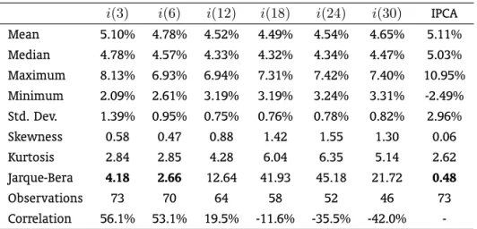
Table 1: Descriptive statistics – BEIR and IPCA
i(3) i(6) i(12) i(18) i(24) i(30) IPCA
Mean 5.10% 4.78% 4.52% 4.49% 4.54% 4.65% 5.11% Median 4.78% 4.57% 4.33% 4.32% 4.34% 4.47% 5.03% Maximum 8.13% 6.93% 6.94% 7.31% 7.42% 7.40% 10.95% Minimum 2.09% 2.61% 3.19% 3.19% 3.24% 3.31% -2.49% Std. Dev. 1.39% 0.95% 0.75% 0.76% 0.78% 0.82% 2.96% Skewness 0.58 0.47 0.88 1.42 1.55 1.30 0.06 Kurtosis 2.84 2.85 4.28 6.04 6.35 5.14 2.62 Jarque-Bera 4.18 2.66 12.64 41.93 45.18 21.72 0.48
Observations 73 70 64 58 52 46 73
Correlation 56.1% 53.1% 19.5% -11.6% -35.5% -42.0%
-This table presents some descriptive statistics of the break-even inflation (i(τ), τ = 3, 6, 12, 18, 24, 30) and the rate of change of the consumer price index (IPCA). The skewness of a symmetric distribution is zero. Positive skewness means that the distribution has a long right tail and negative skewness implies that the distribution has a long left tail. The kurtosis of the normal distribution is 3. If the kurtosis exceeds 3, the distribution is peaked (leptokurtic) relative to the normal; if the kurtosis is less than 3, the distribution is flat (platykurtic) relative to the nor-mal. Under the null hypothesis of a normal distribution, the Jarque-Bera statistic is distributed as chi-squared with 2 degrees of freedom. Boldface values mean significance at a 95% confidence level. The bottom row shows the correlation coefficients between the break-even inflation and the realized inflation.
Table 1 presents some descriptive statistics of the BEIR and IPCA. The averages of the IPCA and BEIR for all horizons are around 5%. Both the BEIR and the realized inflation are leptokurtic with a positive skewness (long right tail). The Jarque-Bera statistic indicates that the 3-month and 6-month BEIR and the IPCA appear to be normally distributed. This is a sign that the BEIR can better explain realized inflation over a short horizon than a long horizon. This sign will be confirmed in the empirical exercise presented in Section 4. The correlation coefficients between the BEIR and realized inflation (the bottom row of Table 1) are positive for the horizons of 3, 6 and 12 months and negative for the horizons of 18, 24, and 30 months. Figure 1 depicts the time evolution of the BEIR and the rate of change of the IPCA from April 2005 to April 2011. Note that the BEIR term structure is almost everywhere upward sloping. Moreover, the BEIR and IPCA exhibit no trend.12
11These data are for April 2011. For more information about the Brazilian Treasury bond market, see the website of the Central
Bank of Brazil,http://www.bcb.gov.br/?english.
12We opt to calculate the descriptive statistics presented in Table 1 only with the data used in the estimation of Eq. (1). Thus, the
Figure 1: BEIR and IPCA
-.04 -.02 .00 .02 .04 .06 .08 .10 .12
II III IV I II III IV I II III IV I II III IV I II III IV I II III IV I II
2005 2006 2007 2008 2009 2010 2011
3M 6M 12M 18M
24M 30M IP CA
Figure 1: BEIR and IPCA
This figure contains time series of the 3-, 6-, 12-, 18-, 24-, 30-month BEIR and the rate of change of the IPCA from April 2005 to April 2011. The BEIR is the difference between the nominal and real yields. The IPCA is the main Brazilian consumer price index.
4. EMPIRICAL RESULTS
In order to provide robust results, we estimate Eq. (1) using three different methods. First we adopt an OLS procedure. Next, we introduce instrumental variables to control for endogeneity. In this case, the model is estimated using TSLS and GMM with the variance-covariance matrix computed as suggested by Newey e West (1987). The instrument specification isit−1(τ)for TSLS andit−1(τ),it−2(τ)and
it−3(τ)for GMM (τ = 3, 6,12, 18, 24, 30). Tables 2, 3 and 4 report the estimates ofc1andc2, the
standard deviations, the correctedR2
, and theF-statistic of the joint hypothesisc1 = 1andc2 = 0
for the OLS, TSLS and GMM methods, respectively.13
Note first that the estimates are very similar across the different estimation strategies, which indi-cates that our results are robust. The slopec1is significant for the horizons of 3, 6, 24 and 30 months.14
Hence, in the short and long term, the BEIR contains some information about future inflation. However, moving from the short to the long horizon, we can easily observe a distinct link between the BEIR and future inflation. For the horizons of 3 and 6 months, theF-statistic of the joint hypothesisc1= 1and
c2 = 0shows that the BEIR is an unbiased estimator of future inflation. In other words, we cannot
13To check the consistency of OLS estimators, we perform the Durbin-Wu-Hausman test (see Ruud, 1984). We find no significant
difference among OLS, TSLS and GMM. Nevertheless, we opt to report the TSLS and GMM estimations in order to provide robust results.
14Apart from the estimate ofc
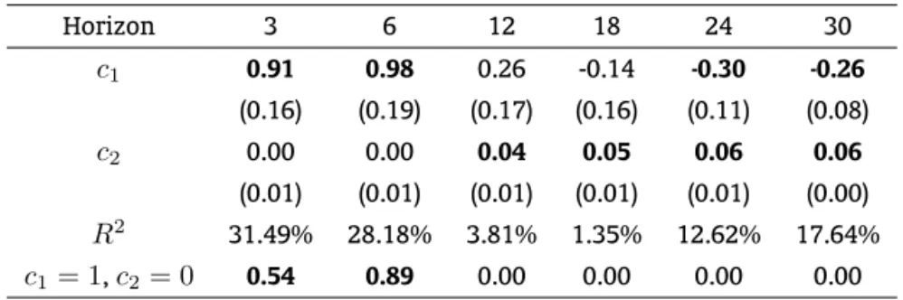
Table 2: OLS results ofht(τ) =c1it(τ) +c2+ǫt+τ
Horizon 3 6 12 18 24 30
c1 0.91 0.98 0.26 -0.14 -0.30 -0.26
(0.16) (0.19) (0.17) (0.16) (0.11) (0.08)
c2 0.00 0.00 0.04 0.05 0.06 0.06
(0.01) (0.01) (0.01) (0.01) (0.01) (0.00) R2
31.49% 28.18% 3.81% 1.35% 12.62% 17.64%
c1= 1,c2= 0 0.54 0.89 0.00 0.00 0.00 0.00
This table presents the OLS estimates ofht(τ) =c1it(τ) +c2+ǫt(Eq. (1) in the paper) for the horizons of 3, 6, 12, 18, 24 and 30 months. Here,it(τ)denotes the BEIR at timetand horizonτ, andht(τ)denotes the consumer price index (IPCA) accumulated betweentandt+τ. The bottom row shows theF-statistic of the joint hypothesisc1 = 1andc2 = 0. Numbers in parentheses denote standard errors. Boldface values mean significance at a 95% confidence level.
reject the BEIR version of the expectation hypothesis.15 On the other hand, for the horizons of 24 and
30 months, the relationship between the BEIR and future inflation is negative.16 Though peculiar, this
finding simply suggests that the expectation hypothesis fails over long horizons. Therefore, the linear relation of Eq. (1) probably cannot accommodate the link between the BEIR and future inflation. A more general specification is necessary in this case. The assumption of constant risk premium can be relaxed, implying a time-varying inflation risk premium for long horizons. This result is consistent with pre-vious empirical evidence. For example, Grishchenko e Huang (2010) document that although the U.S. 10-year inflation risk premium is around zero on average, it is time-varying.
For medium horizons, the coefficientc1 is not significant andR2 is very low. Moreover, theF
-statistic rejects the joint hypothesis c1 = 1 and c2 = 0. This means that the BEIR does not have
information about the 12- and 18-month ahead inflation. We have difficulties to interpret the constant c2 as an inflation risk premium when c1 is statistically different from 1. Nevertheless, since c2 is
significant, ranging between 400 to 700 basis points for medium and long horizons, we can conjecture that investors require a high reward to hold inflation-linked bonds with maturities greater than one year.
In a nutshell, apart from the short horizon, we present evidence that the BEIR fails to correctly predict subsequent movements in inflation. Although the aim of this work is not to examine the causes of this failure, we can imagine some reasons. First, we have only five years of data. Despite the fact our sample size is compatible with that found in other empirical finance studies of emerging economies (see, for instance, Pan e Singleton, 2008, Almeida e Vicente, 2009), we believe that a larger dataset would provide more accurate results. Second, the Brazilian market can actually be risky, which would imply a high risk premium, explaining the weak relationship between the BEIR and future inflation. Third, the BEIR can be affected by a “clientele effect”, which means that the NTN-B may attract investors with preferences for specific maturities and strong aversion to inflation uncertainty.17 The clientele effect
would thus cause a distortion in the inflation expectation extracted from inflation-index bonds. In
15The BEIR version of the expectation hypothesis states that the inflation risk premium is constant over time. 16These results are consistent with correlation coefficients shown in Table 1.
17The clientele effect is modeled within the preferred-habitat theory. Although this theory was proposed more than a half century
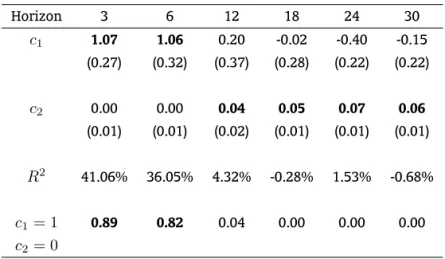
Table 3: TSLS results ofht(τ) =c1it(τ) +c2+ǫt
Horizon 3 6 12 18 24 30
c1 1.07 1.06 0.20 -0.02 -0.40 -0.15
(0.27) (0.32) (0.37) (0.28) (0.22) (0.22)
c2 0.00 0.00 0.04 0.05 0.07 0.06
(0.01) (0.01) (0.02) (0.01) (0.01) (0.01)
R2
41.06% 36.05% 4.32% -0.28% 1.53% -0.68%
c1= 1 0.89 0.82 0.04 0.00 0.00 0.00
c2= 0
This table presents the TSLS estimates ofht(τ) =c1it(τ) +c2+ǫt(Eq. (1) in the paper) for the horizons of 3, 6, 12, 18, 24 and 30 months. Here,it(τ)denotes the BEIR at timetand horizon τ, andht(τ)denotes the consumer price index (IPCA) accumulated betweentandt+τ. The instrument specification isit−1(τ)(τ = 3,6,12,18,24,30) and standard errors are computed by the Newey-West estimator. The bottom row shows theF-statistic of the joint hypothesisc1= 1 andc2= 0. Numbers in parentheses denote standard errors. Boldface values mean significance at a 95% confidence level.
Brazil, the typical buyers of inflation-index bonds are pension funds, for the purpose of hedging their inflation-linked liabilities. In July 2010, pension funds held 33% of NTN-B outstanding and only 5% of LTN and NTN-F outstanding.
5. CONCLUSION
We proposed a model free procedure to assess the relationship between the break-even and future inflations. We showed that the break-even inflation is informative about future inflation over horizons of 3, 6, 24 and 30 months. For the 3- and 6-month horizons, besides being informative, break-even inflation is an unbiased estimator as well. However, over the horizons of 24 and 30 months, the rela-tionship between the break-even and future inflations is negative. On the other hand, for the horizons of 12 and 18 months, break-even inflation has almost no power to explain future inflation. These results indicate that policymakers and market participants should be very careful in using break-even inflation as a proxy for future movements in price indexes.
Table 4: GMM results ofht(τ) =c1it(τ) +c2+ǫt
Horizon 3 6 12 18 24 30
c1 1.17 1.01 0.38 0.03 -0.24 0.05
(0.25) (0.31) (0.23) (0.25) (0.21) (0.17)
c2 -0.01 0.00 0.03 0.05 0.06 0.05
(0.01) (0.01) (0.01) (0.01) (0.01) (0.01)
J-statistic 0.41 0.23 0.22 0.19 0.13 0.12
c1 0.79 1.00 0.02 0.00 0.00 0.00
c2= 0
This table presents the GMM estimates ofht(τ) =c1it(τ) +c2+ǫt(Eq. (1) in the paper) for the horizons of 3, 6, 12, 18, 24 and 30 months. Here,it(τ)denotes the BEIR at timetand horizon τ, andht(τ)denotes the consumer price index (IPCA) accumulated betweentandt+τ. The instrument specification isit−1(τ),it−2(τ)andit−3(τ)(τ = 3,6,12,18,24,30) and standard errors are computed by the Newey-West estimator. TheJ-statistic is thep-value of the test for over-identifying restrictions. The bottom row shows theF-statistic of the joint hypothesisc1= 1 andc2= 0. Numbers in parentheses denote standard errors. Boldface values mean significance at a 95% confidence level.
BIBLIOGRAPHY
Almeida, C. & Vicente, J. (2009). Identifying volatility risk premia from fixed income Asian options.
Journal of Banking & Finance, 33:652–661.
Ang, A., Bekaert, G., & Wei, M. (2008). The term structure of real rates and expected inflation.Journal of Finance, 63:797–849.
Bernanke, B. (2004). What policymakers can learn from asset prices. InSpeech Before the Investment Analyst Society of Chicago. April 15, available athttp://www.federalreserve.gov/boarddocs/ speeches/2004/20040415/default.htm.
Campbell, J. & Shiller, R. (1991). Yield spreads and interest rate movements: A bird’s eye view. Review of Economic Studies, 58:495–514.
Christensen, B. J. & Prabhala, N. R. (1998). The relation between implied and realized volatility. Journal of Financial Economics, 50:125–150.
D’Amico, S., Kim, D., & Wei, M. (2008). Tips from TIPS: The informational content of Treasury inflation-protected security prices. Working Papers 248, BIS.
Evans, M. D. (1998). Real rates, expected inflation, and inflation risk premia. Journal of Finance, 53:187– 218.
García, J. & Werner, T. (2010). Inflation risks and inflation risk premia. Working Paper 1162, European Central Bank.
Greenwood, R. & Vayanos, D. (2010). Price pressure in the bond market.American Economic Review, P&P, 100:585–590.
Grishchenko, O. & Huang, J. (2010). Inflation risk premium: Evidence from the TIPS market. Working paper, Penn State. Available athttp://www.personal.psu.edu/ovg1/.
Hördahl, P. (2008). The inflation risk premium in the term structure of interest rates. BIS Quarterly Review, pages 23–38.
Joyce, M., Lildholdt, P., & Sorensen, S. (2010). Extracting inflation expectations and inflation risk premia from the term structure: A joint model of the UK nominal and real yield curves. Journal of Banking & Finance, 34:281–294.
Newey, W. K. & West, K. D. (1987). A simple, positive semi-definite, heteroskedasticity and autocorrela-tion consistent covariance matrix. Econometrica, 55:703–708.
Pan, J. & Singleton, K. (2008). Default and recovery implicit in the term structure of sovereign CDS spreads. Journal of Finance, 63:2345–2384.
Ruud, P. A. (1984). Tests of specification in econometrics.Econometric Reviews, 3:211–242.
Svensson, L. (1994). Monetary policy with flexible exchange rates and forward interest rates as indica-tors. Technical report, Institute for International Economic Studies, Stockholm University.