A risk- and cost-related approach for the global seismic safety assessment of existing buildings

A risk- and cost-related approach for the global seismic

safety assessment of existing buildings

Romão, X.

Faculdade de Engenharia da Universidade do Porto, Porto, Portugal

Delgado, R.

Faculdade de Engenharia da Universidade do Porto, Porto, Portugal

Costa, A

Universidade de Aveiro, Aveiro, Portugal

SUMMARY:

A probabilistic methodology is proposed to assess the seismic safety of a building using global performance metrics and to determine if it conforms to a given limit state. The performance metrics are the probability of occurrence of the limit state, the corresponding expected loss associated to the repair of the building, and the corresponding number and type of mechanisms that occur. By considering these parameters, the scope of the limit state definitions of current codes is extended to establish adequate risk- and cost-related limit state definitions. The performance of two reinforced concrete structures is then analysed by the proposed method.

Keywords: safety assessment, risk analysis, loss assessment, existing buildings

1. INTRODUCTION

Probabilistic seismic safety assessment methods are intrinsic to the conceptual framework established by current Performance-Based Earthquake Engineering methodologies. This framework involves key aspects such as the use of adequate methods of analysis to determine building behaviour and the definition of quantifiable targets to measure performance. In this context, a probabilistic methodology that analyses the seismic safety of a building using global performance metrics is proposed to determine if its behaviour conforms to a given limit state.

2. PROBABILISTIC PERFORMANCE ANALYSIS METHODOLOGY

To analyse building performance for a given limit state, the proposed methodology uses the probability of occurrence λ of the limit state, the corresponding loss Lsc associated to the repair of the building, and the corresponding number of structural sections nLS where the limit state mechanism occurs. The term mechanism is considered herein as referring to the occurrence of a limit state in one or in a combination of several structural members. By defining a value for nLS, one establishes a possible scenario for the occurrence of a given limit state. The λ and Lsc performance metrics of each of the msc considered scenarios are then combined to obtain a global performance value representing the expected loss EL over a given reference period of time which can be defined by Eq. (1). Finally, the EL value can be compared with an admissible limit ELadm defined by Eq. (2) where λadm and Lsc adm are global acceptance thresholds defined for λ and Lsc. Recommendations by existing standards can be used to define λadm, while the value of Lsc adm can be set, for example, by the building owner.

, 1 sc m i sc i i EL λ L = =

_∑

adm adm sc adm

The value of λ is estimated by

( )

( )

0 pf x dH x dx dx

λ=

_∫

where H is the earthquake hazard curve defined in terms of a given earthquake intensity measure (IM) and pf is the fragility curve representing the probability of exceeding a given state of performance conditional to a certain value of the IM. The considered formulation of the fragility curve is similar to the IM-based approach referred by Ibarra et al. (2002). With respect to the expected value of the loss

Lsc, its quantification uses the storey-based approach by Ramirez and Miranda (2009) and considers a simplified loss model that only addresses losses due to structural and non-structural damage.

When analysing the evolution of λ and Lsc for increasing values of the number of structural sections nLS where a given mechanism occurs (which can be seen as a proxy for the behaviour of the building), λ and Lsc are seen to have opposite evolution trends (Fig. 1). When nLS increases, λ decreases since higher intensity ground motions (with lower probability of occurrence) are required to reach the limit state capacity at a larger number of sections. On the other hand, the value of Lsc increases since admitting that a larger number of sections can reach the EDP capacity also leads to higher levels of global building damage. Figure 1 also shows the evolution of EL which, as expected, is seen to increase as nLS increases. Based on the value set for ELadm, it is then possible to establish the admissible building performance which corresponds to the largest value of nLS conforming with ELadm.

λ & EL n_LS L_sc λ EL L_sc EL _adm

Figure 1. Evolution of λ, Lsc and EL for increasing values of nLS.

Considering that a suitable earthquake hazard curve defined in terms of the selected earthquake IM is available, the quantification of the probability of occurrence λ of a given limit state according to Eq. (3) requires the adequate definition of the fragility curve pf. As previously referred, the fragility curve is estimated by the IM-based approach (Ibarra et al., 2002) which uses a random variable, termed the IM-capacity (IMC), that represents the ground motion intensity at which a given limit state occurs for the structure under assessment. Several realizations of IMC associated to the selected limit state can then be obtained by analysing the structure under a set of earthquake records using incremental dynamic analysis (IDA) where each record is scaled for increasing intensities until the limit state occurs. The cumulative distribution function (CDF) defined by the statistical distribution of the several IMC realizations represents the fragility curve of the selected limit state. This fragility curve is assumed to be represented by a lognormal CDF which enables it to be written as:

( )

(

)

where Φ

( )

C

IM

η and

C

IM

β are the mean and standard deviation of the distribution, respectively. In this approach,

C

IM

As referred, the loss Lsc associated to the occurrence of a limit state is estimated using the storey-based approach proposed by Ramirez and Miranda (2009). This approach defined loss curves representing the losses of all the individual components of an entire building storey as a function of a selected EDP,

Lsc|EDP. Different curves have been defined to quantify the losses in structural and non-structural components, and different EDPs are also selected depending on the type of component. To quantify the expected loss value associated to the ith building storey, Lsc,i, due to the occurrence of a given limit state, the Lsc|EDP,i curve must be combined with the exceedance probability of the selected EDP at the

ith storey, P EDP

(

)

EDPC values represents the fragility curve of the ith storey EDP associated to the occurrence of the limit state under analysis,

,

C i

EDP

p , which can also be assumed to be represented by a lognormal CDF:

( )

(

)

p edp P EDP EDP edp η

β  ₋    = ≤ = = Φ_{ }   (5) where , ln C i EDP η and , C i EDP

β are the mean and the standard deviation, respectively, of the EDP distribution at the ith storey. The value of Lsc,i can then be obtained by:

(

) (

)

( )

L E L EDP dP EDP edp L x dx

dx η β ∞ ∞ _{ − }   = ⋅ > = ⋅ Φ_{ }  

∫

∫

L represents Lsc|EDP,i for the case where the EDP values correspond to those of EDPC. Finally, the total expected value of the loss Lsc associated to the occurrence of the limit state under analysis is obtained by summing the losses of each storey.

2.1 Definition of the limit states

2.1.1. The limit state of Damage Limitation (DL)

For limit states similar to the DL limit state proposed by EC8-3 (EC8-3, 2005), the fundamental issue is related to the number of structural sections where yielding is admissible so that the structure under analysis can still be considered to conform to this limit state. Therefore, the proposed conformity condition based on risk and loss criteria establishes that the occurrence of the limit state can be accepted in a number of scenarios, as long as the corresponding value of EL is not greater than an

admissible value ELadm,DL. In this case, each scenario corresponds to the situation where a different number nDL of structural sections reaches or exceeds the yield limit. By defining the admissible consequences of reaching this limit state in terms of the ELadm,DL, which is a function of the values set for λadm,DL and Lsc adm,DL, the number of admissible yielding sections is set more rationally. Given the type of global structural performance that must be met for the DL limit state, namely the low level of structural damage that is expected, it is suggested that the previously referred simplified loss model could consider the value of Lsc adm,DL such as to reflect repair costs due to non-structural damage only.

2.1.2. The limit state of Significant Damage (SD)

For limit states involving conditions similar to those of the EC8-3 SD limit state, the definition proposed herein is related to both the number of structural sections where the corresponding deformation limit can be attained so that the structure can still be considered to conform to this limit state, and to the level of deformation that should be defined for such limit value. As for the DL limit state, a conformity condition based on risk and loss criteria is also proposed which establishes that the occurrence of the limit state can be accepted in a number of scenarios, as long as the corresponding value of EL is not greater than an admissible value ELadm,SD. In this case, each scenario corresponds to the situation where a different number nSD of structural sections reaches or exceeds a deformation limit

the expected damage-related costs. The value of ELadm,SD is set as a function of the values defined for

λadm,SD and Lsc adm,SD, where the latter should reflect the maximum admissible cost for the repair of the whole structure. Therefore, in terms of the simplified loss model previously referred, Lsc adm,SD reflects the admissible value of the repair costs of both the structural and the non-structural elements.

2.1.3. The limit state of Near Collapse (NC)

With respect to limit states comprising conditions similar to those of the EC8-3 NC limit state, the proposed definition involves different bounding conditions than those of the previous limit states. Given that, when reaching this limit state, the building is expected to be uneconomic to repair, a bounding condition setting a value for the admissible loss is not considered to be relevant. Hence, the building performance is controlled by limiting the probability of occurrence λ of the limit state to an admissible value λadm,NC, and by defining conditions in terms of the number of sections where a given demand/mechanism is accepted. With respect to this last performance measure, when analysing the occurrence of local (section level) mechanisms, distinction must be made between mechanisms occurring in beams and in columns. Given the larger severity of the consequences due to the failure of a column, the occurrence of the NC limit state at a single section is considered to be enough to reflect a nonconforming structure. On the other hand, for beams, it is considered that the limit state capacity of a mechanism can occur at several sections. In this case, a nonconforming condition is established when the NC limit state occurs in all the beam sections of a given storey. In addition to the local (section level) analysis of the demand, a global analysis of the building behaviour is also carried out for this limit state in order to include the influence of the global yield mechanisms. The proposed approach identifies the occurrence of yield mechanisms by assessing the singularity of an equivalent stiffness matrix representing the current state of the building behaviour. This approach is defined by the following steps which are carried out at each time increment of the nonlinear dynamic analysis:

• Step 1 - Check the behaviour state of each structural section to determine if its current loading state is located in a positive or negative post-yield loading branch of the section behaviour path. Sections meeting this condition are termed active yielding sections.

• Step 2 - If one or more active yielding sections are found, an equivalent elastic Euler-Bernoulli stiffness matrix of the structure Keq is formulated with zero-stiffness terms assigned to the flexural terms of those sections.

• Step 3 - If matrix Keq is singular, a situation that represents an unstable structure, the configuration of active yielding sections under consideration is that of a yield mechanism and the corresponding IM value of the ground motion is recorded.

With this procedure, it is then possible to identify any type of yield mechanism taking into account the correlation of the behaviour between the components forming the mechanism and accounting only for sections actively loaded in the post-yield stiffness at each time increment of the analysis.

2.2. Accounting for the uncertainty in the limit state capacities

As referred in Jalayer et al. (2007), the uncertainty associated to the modelling of member limit state capacities has a significant contribution to the probability of occurrence λ of a given limit state since the average capacity estimates provided by the referred expressions are known to have a large uncertainty (fib, 2003a; fib, 2003b). In this case, the uncertainty in the limit state capacities can be associated to the modelling error deriving from the proposed capacity formulas as well as to the variability of the mechanical parameters entering those formulas (Jalayer et al. 2007). Among the different methods which are available to account for this uncertainty component (e.g. see Jalayer et al., 2007), the selected approach assumes that limit state capacities C can be modelled according to:

ˆ UC

C= ⋅C ε (7)

where ˆC is the estimate given by the referred semi-empirical expressions, and εUC is a lognormal random variable with unit median and a dispersion βUC accounting for the variability sources previously mentioned. In order to reflect the section-level limit state capacity uncertainty at the system level, i.e. in the uncertainty associated to the estimate of IMC, the possible correlation between the

capacities of different sections must be accounted for. To address this issue, an approach similar to the one proposed by Jalayer et al. (2007) is considered herein. Therefore, it is assumed that for a given mechanism (e.g. yield deformation, shear failure) the corresponding limit state capacities of all members are fully correlated. On the other hand, for a given member, the limit state capacities of different mechanisms are considered to be uncorrelated. Given this assumption, the effect of this uncertainty on the estimate of IMC can be included by sampling different realizations of the individual member capacities using Eq. (7) which are then paired with the IDA curves obtained from the considered earthquake ground motions. Therefore, for a given IDA curve, an array of member capacities (i.e. a number of realizations, nUC, of the capacities for each member) is established and each sample of capacities (i.e. one realization of the capacity of each member) will lead to a different realization of the IMC associated to the limit state under analysis. Using this approach, the quantification of parameters C IM η and C IM

β which characterize the limit state fragility curve, Eq. (4), are now able to account for the uncertainty in the member capacities.

2.3. Stepwise description of the proposed methodology

Based on the individual features addressed over the previous sections, the sequence of steps involved in the presented probabilistic methodology for the analysis of building performance is described in the following. The proposed method assumes that a set of ngm IDA curves with an adequate number of IM levels have been obtained from the analysis of the structure subjected to ngm ground motion records scaled to those IM levels. After selecting the limit state for which the performance of the structure is to be assessed, the following steps must then be carried out:

• Step 1 - Define the mechanism for which seismic safety will be analysed.

• Step 2 - Define a value for nUC (the number of realizations of the capacity of each member) and sample nUC values of εUC from its distribution.

• Step 3 - Select a value for nLS (the number of sections where the limit state mechanism occurs). • Step 4 - Select a value of εUC from those sampled in Step 2.

• Step 5 - Select one IDA curve from the set of ngm curves. • Step 6 - Select the first IM level from the chosen IDA curve. • Step 7 - Determine

(

)

UC

D C

ρ= ⋅ε for all the nsec sections of the structure. • Step 8 - Determine the number of sections nρ>1 with ρ values larger than 1.0.

• Step 9 - If nρ>1 < nLS, select the next IM level and repeat the procedure from Step 7; if nρ>1 ≥ nLS,

record the IM level, which corresponds to a realization of IMC (the ground motion IM at which the limit state occurs), and proceed to the next IDA curve to repeat the procedure from Step 6. • Step 10 - After going through all the IDA curves, the procedure is repeated from Step 5 for a

different value of εUC, until the whole nUC values have been considered.

• Step 11 - Define the limit state fragility curve by Eq. (4) based on the realizations of IMC. • Step 12 - Determine the probability of occurrence λ of the limit state by Eq. (3).

• Step 13 - Characterize the fragility curves of the selected EDP of each storey for the storey-based loss quantification by Eq. (5).

• Step 14 - Determine the expected value of the loss of each storey by Eq. (6). • Step 15 - Determine the value of the loss Lsc of the limit state scenario.

After these steps, the triplet (nLS; λ; Lsc) defines a limit state performance scenario. The building performance quantification procedure is then repeated from Step 4 for a different value of nLS. In order to obtain an adequate representation of the building performance evolution for different nLS values, it is suggested that the analysis starts by setting nLS equal to one and that subsequent repetitions of the procedure increase it by single units. The several performance triplets are then combined to obtain EL according to Eq. (1). The value of EL is then analysed in light of the limit defined by ELadm to determine which combination of scenarios is admissible for the current limit state. It is noted that additional verifications may be carried out in Step 10 if provisions other than checking the nρ>1

3. EXAMPLE APPLICATION OF THE PROPOSED METHODOLOGY 3.1 Description of the selected structures and of the additional data required

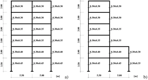
The selected reinforced concrete (RC) structures are the six-storey frames presented in Figs. 2a) and b) and referred as REG6 and IRREG6. The column cross section dimensions are also presented in Fig. 2 and all the beams are 0.30×0.50 m2. Additional information concerning the frame characteristics can be found in Ferracuti et al. (2009). Details about the structural modelling, the analysis procedure and the quantification of the demand parameters are discussed in Romão et al. (2011) and Romão (2012).

0.30x0.30 0.30x0.30 0.30x0.35 0.30x0.35 0.30x0.40 0.30x0.45 0.30x0.30 0.30x0.30 0.30x0.35 0.30x0.35 0.30x0.40 0.30x0.45 0.30x0.30 0.30x0.30 0.30x0.35 0.30x0.35 0.30x0.40 0.30x0.45 3 .0 0 3 .0 0 3 .0 0 3 .0 0 3 .0 0 3 .5 0 5.00 _[m] 5.50 a) 3 .0 0 3 .0 0 3 .0 0 3 .0 0 3 .0 0 3 .5 0 0.30x0.30 0.30x0.30 0.30x0.30 0.30x0.30 0.30x0.30 0.30x0.35 0.30x0.35 0.30x0.35 0.30x0.35 0.30x0.35 0.30x0.40 0.30x0.40 0.30x0.45 0.30x0.45 5.00 5.50 _[m] b) Figure 2. Elevation views of the REG6 (a) and of the IRREG6 (b) frames.

The member ductile capacities were defined according to the EC8-3 admissible DL, SD and NC member chord rotations, θDL, θSD and θNC, respectively, while brittle capacities are characterized by the admissible EC8-3 NC shear force VNC. To account for the uncertainty in θDL according to Eq. (7), fifty

εUC values are sampled from its distribution, where the dispersion βUC for θDL is considered to be 0.36 (fib, 2003b). To quantify the NC chord rotation capacity θNC, the semi-empirical expression proposed by EC8-3 was considered. To account for the uncertainty in θNC according to Eq. (7), fifty εUC values are sampled from its distribution, where the dispersion βUC for θNC is 0.90 (fib, 2003b). For the SD limit state, EC8-3 states that the chord rotation capacity θSD is 0.75θNC. Since θSD is a function of θNC, the uncertainty in θSD is that of θNC. To account for the uncertainty in VNC according to Eq. (7), fifty εUC values are sampled from its distribution, where the dispersion βUC for VNC is 0.14 (fib, 2003a).

The seismic demand considered for each structure consisted of a suite of fifty real ground motions extracted from the Pacific Earthquake Engineering Research Center NGA database according to the criteria referred in Romão et al. (2011) and Romão (2012). Each structure was analysed using a multi-stripe analysis where the selected ground motions are scaled for increasing values of the 5% damping spectral acceleration ordinate of the ground motion for the fundamental period of the structure (which is the selected IM and is referred to as Sa hereon) until the selected limit state is attained. In order to define the earthquake hazard curve required for Eq. (3), seismic hazard data was obtained for the Sa values of the considered structures, and for a reference period of one year, in order obtain results in terms of annual performance of the structures. Additional details can be found in Romão (2012). The expected loss value associated to the ith building storey, Lsc,i, is quantified using the Lsc|EDP structural and non-structural loss curves for mid-rise RC interior frames of an office building defined by Ramirez and Miranda (2009). In order to simplify the proposed example applications, only non-structural losses associated to inter-storey drift-sensitive non-structural components are considered herein. With respect to the selected values of the admissible expected losses ELadm defined by Eq. (2), values were set for the admissible probability of occurrence of the considered limit states,

λadm, and for their expected repair costs, Lsc adm. For the case of λadm, it is referred that, for existing structures, current standards and/or available technical documents on the subject do not have definitive proposals on this matter. Therefore, the λadm values considered herein were defined as a reduction of

the target reliability values for new structures proposed by the JCSS (2001) for a one year reference period and for ultimate limit states. This is based on the fact that achieving a higher reliability level in existing structures has a higher cost when compared to that of structures under design. Hence, the λadm values presented in Table 1 were considered for the selected limit states, based on those proposed by the JCSS (2001) for the higher category of the relative cost of implementing safety measures. These

λadm values are defined for the reference period of one year and were associated to small, moderate and large risks to life and economic consequences for the limit states of DL, SD and NC, respectively. With respect to the selected values for the admissible expected repair costs, Lsc adm, the considered limit values correspond to average repair costs of all the building storeys. Therefore, a value of 10% was assumed for the DL limit state (considering only losses associated to inter-storey drift-sensitive non-structural components) and a value of 25% was assumed for the SD limit state (considering losses associated to inter-storey drift-sensitive non-structural components and losses to structural components). Considering the proposed values of λadm and Lsc adm for the limit states of DL and SD, the corresponding values of ELadm set by Eq. (2) are then 10-4 and 5×10-5, respectively.

Table 1. Considered values for λadm for the selected limit states.

Limit state DL SD NC

λadm 0.001 0.0002 0.0001

3.2 Results of the probabilistic performance analysis

3.2.1 Results for the DL limit state

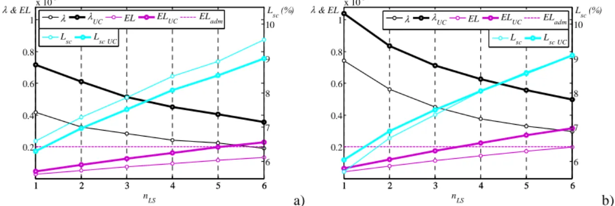
Based on the IDA curves obtained for all the considered ground motions, the performance of the REG6 and IRREG6 structures was analysed for nLS values of one to six. The calculated performance metrics λ and Lsc are presented in Fig. 3. For a more direct analysis about the influence of the modelling error of the capacity model, the performance results of both structures are presented for the situation where the uncertainty of the component capacities is neglected and also for the situation where it is accounted for. In addition to these results, Fig. 3 also presents the cumulative sum of EL up to each value of nLS along with the selected value for ELadm. Parameters λUC, Lsc UC and ELUC are the values of λ, Lsc and EL obtained when the uncertainty of the component capacities is considered.

1 2 3 4 5 6 0.2 0.4 0.6 0.8 1 x 10-3 λ & EL n_LS 1 2 3 4 5 6 6 7 8 9 10 L_sc (%) λ λUC EL ELUC ELadm L_sc L_scUC a) 1 2 3 4 5 6 0.2 0.4 0.6 0.8 1 x 10-3 λ & EL n_LS 1 2 3 4 5 6 6 7 8 9 10 L_sc (%) λ λUC EL ELUC ELadm L_sc L_scUC b) Figure 3. Performance of the REG6 (a) and the IRREG6 (b) structures for the DL limit state.

The results of the REG6 and IRREG6 structures when the uncertainty of the capacity models is not considered indicate that performance scenarios up to nLS equal to six can be seen to lead to acceptable values of EL. On the other hand, allowing for the uncertainty of the component capacities can be seen to increase the risk considerably: the λUC values are 30% to 75% larger than the λ values. On the other hand, the uncertainty effects on the expected costs are different. For structure REG6, the uncertainty of the component capacities reduces the expected costs: Lsc UC is, on average, 5% lower than Lsc. For structure IRREG6, the uncertainty increases the expected costs for the nLS cases of one to three (Lsc UC is 6% larger than Lsc when nLS = 1) while there is virtually no difference between Lsc UC and Lsc for the remaining nLS cases. With respect to the performance of the REG6 and the IRREG6 structures, the

changes from λ to λUC and from Lsc to Lsc UC also modify the number of performance scenarios up to which the value of EL is found to be admissible. For REG6, the performance measure ELUC is admissible up to nLS =5, while for IRREG6 the performance is only acceptable up to nLS = 3. Hence, accounting for the uncertainty in the component capacities can be seen to have a significant influence on the acceptable performance of the structures, namely due to the significant increase of λ to λUC.

3.2.2 Results for the SD limit state

The performance metrics λ, Lsc and EL obtained for the limit state of SD for the REG6 and the IRREG6 structures are presented in Fig. 4 for nLS values of one to four, for the cases where the uncertainty of the component capacities is neglected and is accounted for, and considering the chord rotation capacity defined by θSD. As for the DL limit state, λUC, Lsc UC and ELUC are the values of λ, Lsc and EL obtained when considering the uncertainty of the component capacities.

1 2 3 4 1 2 3 x 10-4 λ & EL n_LS 1 2 3 4 10 15 20 25 L_sc (%) λ λ_UC EL EL_UC EL_adm L_sc L_scUC a) 1 2 3 4 1 2 3 x 10-4 λ & EL n_LS 1 2 3 4 10 15 20 25 L_sc (%) λ λUC EL ELUC ELadm L_sc L_scUC b) Figure 4. Performance of the REG6 (a) and the IRREG6 (b) structures for the SD limit state.

From the results presented in Fig. 4, including the uncertainty of the component capacities increases the risk considerably: the λUC values are 50% to 120% larger than the λ values. On the other hand, as observed for the limit state of DL, the influence of the uncertainty on the expected costs has an opposite effect: the Lsc UC values are 6% to 15% lower than the Lsc values. As opposed to what was observed for the DL limit state, accounting for the uncertainty in the component capacities reduces the expected costs of both structures and for all the nLS cases. As for the DL limit state, accounting for the uncertainty in the component capacities also modifies the number of performance scenarios up to which the value of EL is found to be admissible. When uncertainty is not considered, the results of the REG6 and IRREG6 structures indicate that performance scenarios up to nLS equal to four will to lead to acceptable values of EL. On the other hand, when uncertainty is considered, the performance measure ELUC of REG6 is only admissible for nLS = 1, while for IRREG6 the performance is

acceptable up to nLS = 3. Unlike for the DL limit state, the results of Fig. 4 indicate that λ values are

globally higher for REG6 than for IRREG6. This situation arises from the fact that, for REG6, larger deformation demands occur at the bottom columns, while for IRREG6 the larger deformation demands are obtained for the columns immediately above the setback. Since the limit state capacity of the bottom columns of REG6 is smaller than that of the IRREG6 third storey columns, REG6 reaches the limit state condition for lower IM values, thus leading to a larger value of λ.

Results for the NC limit state

Given the assumptions established in Section 2.1.3, only λ values are presented to analyse the performance of the REG6 and the IRREG6 structures for the limit state of NC. With respect to the limit state conditions also defined in Section 2.1.3, it was found that the occurrence of a NC limit state nonconforming condition in all of the beam sections of a given storey was not a governing scenario in any of the cases analysed, both in terms of the rotation capacity θNC and of the shear force capacity

VNC. Furthermore, the occurrence of the shear force capacity VNC in columns was not a governing scenario also. Hence, the NC limit state performance of the structures was governed by the NC rotation capacity in columns and by the development of global yield mechanisms. To observe the importance of each of these nonconforming conditions, the following five scenarios were analysed:

• Scenario 1 (S1) - Only the column rotation demand is controlled and the uncertainty of the rotation capacities is not considered;

• Scenario 2 (S2) - Only the column rotation demand is controlled and the uncertainty of the rotation capacities is accounted for;

• Scenario 3 (S3) - Only the development of global yield mechanisms is controlled;

• Scenario 4 (S4) - Both the column rotation demand and the development of global yield mechanisms are controlled and the uncertainty of the rotation capacities is not considered; • Scenario 5 (S5) - Both the column rotation demand and the development of global yield

mechanisms are controlled and the uncertainty of the rotation capacities is accounted for. Based on the definition of these scenarios, it is referred that the uncertainty in the development of the global yield mechanisms due to the uncertainty in the value of the yield curvature of the components has not been considered. The λ values which correspond to the performance results of REG6 and IRREG6 for the five scenarios are presented in Table 2. The presented results indicate that only scenarios that do not involve the development of global yield mechanisms are able to conform to the condition λ ≤ λadm = 0.0001. As can be observed, when the development of global yield mechanisms is considered, the λ values almost duplicate. This fact clearly emphasizes the importance of considering this type of condition when analysing structural safety and performance under earthquake loading. When considering the scenario S4, the analysis of the results of both structures indicated that the limit state capacity was governed by the rotation demand in a column for only one ground motion. This situation implies that the median of the Sa,C realizations has a 0.2% reduction from the scenario S3 to the scenario S4 and that the standard deviations of the log of the Sa,C realizations has a reduction of about 2.7%. The latter reduction is the governing factor and leads to the slight decrease of the λ value from S3 to S4. When comparing the scenarios S3 and S5, the uncertainty in the rotation capacities plays a larger role and reduces the median of the Sa,C realizations by 1.9%. Although there is also a 1.9% reduction of the standard deviations of the log of the Sa,C realizations from S3 to S5, the shift of the median is now the governing factor leading to the increase of the λ value from S3 to S5.

Table 2. Performance results of REG6 and IRREG6 for the NC limit state considered scenarios.

Scenario S1 S2 S3 S4 S5

λ - REG6 3.13E-5 4.52E-5 1.27E-4 1.26E-4 1.33E-4

λ - IRREG6 4.95E-5 7.02E-5 1.91E-4 1.90E-4 2.00E-4

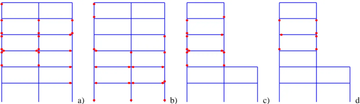
With respect to the global yield mechanisms that were found when analysing this limit state, the unpredictability of their configurations and the importance of using a technique such as the one presented in Section 2.1.3 should be emphasized. In order to illustrate some of the global yield mechanisms that were found, Fig. 5 presents two examples for each structure. Although the cases presented in Figs. 5a) and c) ended up being controlled by a familiar mechanism (a soft-storey mechanism), the cases of Figs. 5b) and d) are less common. These results indicate clearly that approaches such as the one referred in Jalayer et al. (2007) that require the identification of the global yield mechanism configurations may not be practical to use due to the multitude of possibilities.

a) b) c) d)

Figure 5. Examples of global yield mechanisms that were found when analysing the NC limit state.

Finally, it is noted that the λ values of IRREG6 are again higher than those of REG6. For the S1 and the S2 scenarios, this situation occurs since the contribution of the REG6 upper storeys to the lateral

demand is now much more significant, thus reducing the bottom storey demand concentration referred previously. Since, for IRREG6, the larger deformation demands still occur at the columns immediately above the setback, IRREG6 was seen to reach the limit state condition for IM values lower than those of REG6, thus leading to higher λ values. When the development of global yield mechanisms governs the performance, IRREG6 was found to reach the limit state condition for IM values lower than those of REG6 since less yielding sections are usually required to develop the referred mechanisms.

CONCLUSIONS

A probabilistic methodology was proposed to analyse the seismic performance of existing buildings using global metrics to determine if the behaviour conforms to a given limit state. The performance metrics are the probability of occurrence λ of the limit state, the corresponding loss Lsc associated to the repair of the building, and the corresponding number nLS and type of mechanisms that occur. Each case of nLS establishes a scenario corresponding to the occurrence of the limit state. The λ and Lsc values of each considered scenario are then combined to define a global performance value that represents the expected loss EL associated to that limit state. To consider λ, Lsc and the occurrence of several scenarios of the mechanisms as performance parameters, an update of existing limit state definitions was performed. Alternative proposals were defined based on the EC8-3 descriptions to establish risk- and cost-related limit state definitions. These were then used to analyse the performance of two RC structures by the proposed method for the limit states of DL, SD and NC.

To emphasize the influence of the modelling error of the selected capacity models, the performance assessment results were presented for the situation where the uncertainty of the component capacities is neglected and for the situation where it is accounted for. A global analysis of the performance results indicates that, with respect to the situation where the uncertainty of the component capacities is not considered, allowing for such uncertainty increases the risk considerably (e.g. more than duplicating the risk in some cases) while leading to moderate reductions of the expected losses. In the overall, the proposed methodology was able to determine admissible performance scenarios that go beyond the code definitions, which may allow for a rational decision-making process about the need to retrofit or strengthen a given structure. In this context, the analysis carried out for the NC limit state emphasized the importance of considering the potential occurrence of global yield mechanisms, as well as that of having a process able to account for the unpredictability of their configurations.

REFERENCES

Ferracuti, B., Pinho, R., Savoia, M. and Francia, R. (2009) Verification of displacement-based adaptive pushover through multi-ground motion incremental dynamic analyses. Engineering Structures 31:8, 1789-1799. EC8-3 (2005) ENV 1998-3. Eurocode 8: Design of structures for earthquake resistance - Part 3: Assessment and

retrofitting of buildings. European Committee for Standardization, Brussels, Belgium.

fib (2003a) Seismic assessment and retrofit of reinforced concrete buildings. Bulletin nº24, Fédération Internationale du Béton. Lausanne, Switzerland.

fib (2003b) Displacement-based seismic design of reinforced concrete buildings. Bulletin nº25, Fédération Internationale du Béton. Lausanne, Switzerland.

Ibarra, L., Medina, R. and Krawinkler, H. (2002) Collapse assessment of deteriorating SDOF systems. Proceedings of the 12th European Conference on Earthquake Engineering. London, England, UK. Jalayer, F., Franchin, P. and Pinto, P.E. (2007) A scalar damage measure for seismic reliability analysis of RC

frames. Earthquake Engineering and Structural Dynamics 36:13, 2059-2079.

JCSS (2001) Probabilistic assessment of existing structures. Joint Committee on Structural Safety. RILEM Publications S.A.R.L, Bagneux, France.

Ramirez, C. and Miranda, E. (2009) Building-specific loss estimation methods & tools for simplified

performance-based earthquake engineering. Report Nº 171. John A. Blume earthquake engineering research center. Stanford University. Stanford, California, USA.

Romão, X., Costa, A. and Delgado, R. (2011) Assessment of the statistical distributions of structural demand under earthquake loading. Journal of Earthquake Engineering 15:5, 724-753.

Romão, X. (2012) Deterministic and probabilistic methods for structural seismic safety assessment. PhD thesis. Faculty of Engineering of the University of Porto, Portugal.