Analysis of variance of partial diallel tables

INTRODUCTION

The methods of diallel analysis proposed by Jinks and Hayman (1953) and Hayman (1954b, 1958) employ first degree statistics (means) to estimate variances and covari-ances used to assess adequacy of the additive-dominance model and estimate the genetic components of variation and other genetic parameters. Since fitted linear models use second degree statistics (variances and covariances), the approach is less precise in sampling variation terms than analysis of variance.

Variance analysis of diallel tables allows inferences about the significance of genetic components of variation (Hayman, 1954a) using tests based on statistics with known distributions (Searle, 1971; Graybill, 1976). As for the methods proposed by Griffing (1956) and Gardner and Eberhart (1966), and their adaptations to partial diallels (Miranda Filho and Geraldi, 1984; Geraldi and Miranda Filho, 1988), the diallel analysis corresponds to a vari-ance analysis.

This paper presents variance analysis of partial dial-lel tables including parents and their F1 hybrids or F2

gen-erations, according to Hayman’s proposal. Allowing a de-tailed evaluation of dominance in the polygenic systems under study, the analysis assesses specific, varietal and mean heteroses.

METHODOLOGY

Partial diallel analysis, which includes assessing the adequacy of the additive-dominance model from variance analysis of the differences between covariance (W) and vari-ance (V) in the arrays and/or from regression analysis of W on V (Mather and Jinks, 1974) in each group of parents,

makes variance analysis of the partial diallel table redun-dant at many points, since they virtually duplicate infor-mation. Also, several tests in variance analysis are repeti-tive, making them appear insignificant. We will show, how-ever, that they can complement each other, mainly regard-ing specific, varietal and mean heteroses.

Tables I and II show analyses of variance of plot means or totals involving N parents, with n in one group and n’ in the other (n + n’ = N), and their nn’ F1 hybrids or

F2 generations, arranged in a randomized complete block

design. The non-genetic component of the expected mean squares was obtained assuming equal variances for

residu-als associated with observations of the parents (etj) and

their F1 hybrids or F2 generations (ersj) (V(etj) = V(ersj) = σ2_{, for all t, r, s and j; t = 1, ..., N; r = 1, ..., n; s = 1, ..., n’,}

and j = 1, ..., b, where b is the number of replications). The means mL0, mL0, mL1 and mL2, the non-genetic components

E, E’ and E”, the genetic components of the expected mean squares and the other parameters presented throughout the text are defined by Viana et al. (1999, in press). The values p and q are, respectively, n/N and n’/N. Note that the addi-tive genetic components D(1), D(2) and D(3) = (D - p2D(1)

-q2_D

(2))/2pq are estimable.

The treatment sum of squares is:

SSTreatments =

METHODOLOGY

Analysis of variance of partial diallel tables

José Marcelo Soriano Viana1_{, Cosme Damião Cruz}1_{, Antonio Américo}

Cardoso2 _{and Adair José Regazzi}3

Abstract

The theory of variance analysis of partial diallel tables, following Hayman’s proposal of 1954, is presented. As several statistical tests yield similar inferences, the present analysis mainly proposes to assess genetic variability in two groups of parents and to study specific, varietal and mean heteroses. Testing the nullity of specific heteroses equals testing absence of dominance. Testing equality of varietal heteroses of the parents of a group is equivalent to testing the hypothesis that in the other group allelic genes have the same frequency. Rejection of the hypothesis that the mean heterosis is null indicates dominance. The information obtained complements that provided by diallel analysis involving parents and their F1 hybrids or F2 generations. An example with the common bean is included.

Departamentos de 1_{Biologia Geral,} 2_{Fitotecnia and} 3_{Informática, Universidade Federal de Viçosa,}

36571-000 Viçosa, MG, Brasil. Send correspondence to J.M.S.V. r

y2_-(y.) _] 2

n + ∑

n’ s = 1ys

2 _]

b[ -(y.) 2

n’

’

+

∑n

r = 1

{b[ ’

]} + b[(y.) 2

n

(y.) 2

n’

+ - (y. + y.) 2

n + n’

’

{bn’[∑

n r = 1

-+

r

y2

.

(y..) 2

n(n’)2

’

]

bn[∑

n’ s = 1

.s

y2 (y..) 2

(n)2_n’

- + b[∑

n r = 1 ∑

n’ s = 1 rs

y2 _{- n’}∑

n r = 1 r

y2

.- n ∑ n’ s = 1y.s

2₊

Table I - Analysis of variance of partial diallel involving parents and their F₁ hybrids arranged in a randomized complete block design.

Source of variation Degrees of freedom e(mean square)

Constant 1

-Blocks b - 1

-Treatments (N + nn’- 1)

parents (N - 1) σ2 _{+ bD}

parents|group 1 n - 1 σ2 _{+ bD}

(1)

parents|group 2 n’- 1 σ2 _{+ bD}

(2)

between groups 1

F₁ hybrids (nn’- 1)

arrays|group 1 n - 1

arrays|group 2 n’- 1

arrays|group 1 x arrays|group 2 (n - 1)(n’- 1)

parents vs. F1 hybrids 1

Error (b - 1)(N + nn’- 1) σ2 _{(bE = bE’)}

error (1) (b - 1)(N - 1) bE

error (2) (b - 1)(nn’- 1) bE’

error (3) (b - 1)

-Total b(N + nn’)

bn’ 4

σ2_{+ (D}

(1) - F(2) + H1(1) - H2)

bn 4

σ2_{+ (D}

(2) - F(1) + H1(2) - H2)

b 4(n - 1)(n’ - 1)

σ2 _{+ [(n’ - 1) D}

(1) + (n - 1) D(2)

-(n - 1) F(1) - (n’ - 1) F(2) + (n’ - 1) H1(1) +

(n - 1) H1(2) - (n - 1) (n’ - 1) H2]

bNnn’ (N + nn’)

σ2_{+ (m}

L1 - pmL0 - qmL0’)2

bnn’ N

σ2_{+ (m}

L0 - mL0’)2

b 4

σ2_{+ (D}

(1) + D(2) - F(1) - F(2) + H1(1) + H1(2) - H2)

= {SSParents|Group 1 + SSParents|Group 2 + SSBetween Groups} + {SSArrays|Group 1 + SSArrays|Group 2 +

SS(Arrays|Group 1 x Arrays|Group 2)} + SS(Parents vs. F1

Hybrids or F2 Generations)

= SSParents + SS(F1 Hybrids or F2 Generations) +

SS(Parents vs. F1 Hybrids or F2 Generation),

where yr and ys are the means of the rth and sth parents and

yrs is the mean of the F1 hybrid or F2 generation derived

from them.

The error (1) sum of squares is obtained from the analysis of variance considering only the parents. The er-ror (2) sum of squares is obtained considering only the

F1 hybrids or F2 generations. The sum of squares due to

the constant is that attributable to the hypothesis that the expectation of the observed variable is null. The block sum of squares is that due to the hypothesis of equality of the block means. Acceptance of this hypothesis im-plies that weighted average of the means of the n parents in one group, n’ parents in the other group and nn’ F1

hy-brids or F2 generations is constant over the b blocks.

Consequently, the genetic effects da and ha are constants

under the various environmental conditions defined by the blocks. The treatment sum of squares is that attribut-able to the hypothesis of equality of the means of the N + nn’ treatments, that is, of the N parents and nn’ F1

hy-brids or F2 generations (H0 : pr = ps = frs or grs, for every r

and s). Its acceptance shows a lack of genetic variability among the parents (θra= θsa, for every r, s and a; a = 1, ..., k, where k is the number of loci in the polygenic system under study).

The sum of squares of parents, of parents of group 1 and of parents of group 2 are, respectively, those due to the hypotheses of equality of the means of the N parents (H0 : θta = θa, for every t and a), n parents (H0 : θra = θa, for

every r and a) and n’ parents (H0 : θsa = θa, for every s and

a). Acceptance of these hypotheses also implies lack of genetic variability. The between groups sum of squares is attributable to the hypothesis H0 : mL0 = mL0. Its

accep-tance shows that the genes are, probably, equally frequent in the two groups of parents (wa = wa, for every a) and,

therefore, that D(1) = D(2) = D(3) = D, F(1) = F(2) = F and H1(1)

= H1(2) = H₁₍₃₎ = H1.

The sum of squares of F1 hybrids or F2 generations

(y..) 2

nn’ ]} + b[ +

(y..) 2

nn’

-(y. + y. + y..) 2

N + nn’

’

] (y. + y.) 2

n + n’

’

’

is due to the hypothesis of equality of the means of the F1 hybrids or F2 generations. Testing this hypothesis is

equivalent to testing absence of variability in the two groups of parents (H0 : θra = θa and θsa = θa, for every r, s

and a). The sum of squares attributable to the hypothesis of equality of the means of the arrays of the parents in group 1 and the sum of squares due to the same hypoth-esis in group 2 is the sum of squares of the arrays within group 1 and group 2, respectively. The test of the hy-pothesis of equality of the means of the arrays within a group tests the hypothesis of equality of the parental genotypes in the group (H0 : θra = θa or H0 : θsa = θa, for

every r or s and for every a). The interaction sum of squares is also a sum of squares attributable to the hy-pothesis of absence of genetic variability in both groups of parents.

The sum of squares of parents versus F1 hybrids and

of parents versus F2 generations are, respectively, the sums

of squares due to the hypotheses:

Thus, testing these hypotheses is not equivalent to testing H0 : h = 0. The equivalence only occurs if wa = wa

or if p = q.

Variance analysis yields detailed assessment of domi-nance in the polygenic system under study. Consider the following hypothesis:

H0(1) : frs - (1/2)(pr + ps) = (1/2)hrs = 0, for every r and s, if

parents and F1 hybrids were evaluated, or

H0(1) : grs - (1/2)(pr+ ps) = (1/4)hrs = 0, for every r and s, if

parents and F2 generations were evaluated.

If there is evidence of genetic variability among the parents, testing the hypothesis H0(1): hrs = 0, for every r and

∑k

a = 1

1 2

H0: mL1 - mL0 = da (wa + wa - 2wa) +

1

2 h = 0

’

∑k

a = 1

1 2

H0: mL2 - mL0 = da (wa + wa - 2wa) +1

4 h = 0

’

Table II - Analysis of variance of partial diallel involving the parents and their F₂ generations arranged in a randomized complete block design. Source of variation Degrees of freedom e(mean square)

Constant 1

-Blocks b - 1

-Treatments (N + nn’- 1)

parents (N - 1) σ2 _{+ bD}

parents|group 1 n - 1 σ2 _{+ bD}

(1)

parents|group 2 n’- 1 σ2 _{+ bD}

(2)

between groups 1

F₂ generations (nn’- 1)

arrays|group 1 n - 1

arrays|group 2 n’- 1

arrays|group 1 x arrays|group 2 (n - 1)(n’- 1)

parents vs. F2generations 1

Error (b - 1)(N + nn’- 1) σ2_{(bE = bE”)}

error (1) (b - 1)(N - 1) bE

error (2) (b - 1)(nn’- 1) bE”

error (3) (b - 1)

-Total b(N + nn’)

bnn’ N

σ2_{+ (m}

L0 - mL0’)2

1 4

H1(2) - 1

4 H2)

σ2_{+ (D}

(1) + D(2)

-b 4

1 2 F(1)

-1 2 F(2) +

1 4 H1(1) +

σ2 ₊bn’

4 (D(1) - F(2) + H1(1) -1

2 1 4

1 4 H2)

σ2 ₊bn

4 (D(2) - F(1) + H1(2) -1

2 1 4

1 4 H2)

σ2 _{+ [(n’ - 1) D}

(1) + (n - 1) D(2)

-F(1) - H1(1) +

(n - 1)

2 F(2) +

(n’ - 1) 2

(n’ - 1) 4 H1(2)

-(n - 1) 4

b 4(n - 1)(n’ - 1)

bNnn’ (N + nn’)

σ2_{+ (m}

L2 - pmL0- qmL0’)2

H2]

4 (n - 1)(n’ - 1)

’

’

s (nullity of the specific heteroses), equals testing the hy-pothesis of absence of dominance in the polygenic system under study (H0(1): ha = 0, for every a). Acceptance of this

hypothesis implies that Fr = Fs = F(1) = F(2) = H1(1) = H1(2) =

H1(3) = H2r = H2s = H2 = hr = hs = h = 0.

Other hypotheses testable in variance analysis are:

for every rand r’(r

≠

for every rand r’(r

≠

for every s and s’(s

≠

for every s and s’(s ≠ s’)

In the presence of genetic variability in the two groups of parents and dominance in the polygenic system under study, with a non-constant ha value, testing hypothesis H0(2) :

hr = hr’ for every r and r’ (equality of the varietal heteroses

of the n parents of a group), is equivalent to testing the hy-pothesis that in the group with n’ parents the allelic genes are as frequent (H0(2): wa = 0, for every a). In the same way,

testing hypothesis H0(3) : hs = hs’, for every s and s’ (equality

of varietal heteroses of n’ parents of the other group), is equivalent to testing the hypothesis that in the group with n parents allelic genes are just as frequent (H0(3) : wa = 0, for

every a). Acceptance of H0(2) implies that D(2) = D(3), F(2) = 0,

H1(1) = H2s = H2 and H1(2) = H1(3). Acceptance of H0(3) implies

that D(1) = D(3), F(1) = 0, H1(1) = H1(3) and H1(2) = H2r = H2. If

the two hypotheses are accepted, then D(1) = D(2) = D(3), F(1) =

F(2) = 0 and H1(1) = H1(2) = H1(3) = H2r = H2s = H2.

Expressing the hypotheses H0(1), H0(2) and H0(3) in terms

of the components of the statistical model results in: H0(1) : trs - (1/2)tr - (1/2)ts = 0, for every r and s (nn’ linear,

estimable and independent parametric functions);

for every r and r’(n - 1 linear, estimable and independent parametric functions);

for every s and s’ (n’- 1 linear, estimable and independent parametric functions),

where trs is the effect of the F1 hybrid or F2 generation

ob-tained from the cross among the rth and sth parents, tr is the

effect of the rth parent and ts is the effect of the sth parent.

The sums of squares attributable to the hypotheses H0(1)(sum of squares of the specific heterosis), H0(2) (sum

of squares of the varietal heterosis in the group with n par-ents) and H0(3) (sum of squares of the varietal heterosis in

the group with n’ parents) may be obtained based on gen-eral linear model theory. Let the linear model Y = Xβ + ε (ε ~ N (Φ,σ2_{I)). The sum of squares due to the hypothesis}

H0 : Hβ = c versus Ha: Hβ≠ c, where H is a full row rank

matrix and Hβ is a set of (rank of H) linear combinations

of the parameters, estimable and independent, is (Graybill, 1976; Searle, 1971):

SS(H0) = (Hβo - c)’[H(X’X) G

H’]-1 (Hβo _{- c),}

with (rank of H) degrees of freedom. A solution of the system of normal equations is βo _{and (X’X)}G is any

gener-alized inverse of X’X. The statistic for the test of hypoth-esis H0 : Hβ = c is:

which, under H0, has an F distribution with (rank of H) and

[b(N + nn’) - (rank of X)] degrees of freedom (Graybill, 1976; Searle, 1971).

Therefore, the sums of squares due to hypotheses H0(1), H0(2) and H0(3) have nn’, (n - 1) and (n’ - 1) degrees of

freedom, respectively. As this approach is unfeasible even for those with knowledge of linear models theory, the fol-lowing formulae should be used (Miranda Filho and Geraldi, 1984):

SS(H0(1)) = SS(H0(4)) + SS(H0(2)) + SS(H0(3)) + SS

(Arrays|Group 1 x Arrays|Group 2)

where y. and y. are the means of the groups with n and n’ parents and y.. is the mean of the F1 hybrids or F2

genera-tions.

The sum of squares attributable to the hypothesis H0(4) : mL1 - (1/2)(mL0 + mL0) = (1/2)h = 0 or H0(4) : mL2

-(1/2)(mL0 + mL0) = (1/4)h = 0, depending on the

popula-tions assessed, is the sum of squares due to the hypoth-esis that the mean heterosis is null (H0(4) : h = 0) (sum of

squares of the mean heterosis). Rejection of the hypoth-esis shows the presence of dominance in the polygenic system under study. The sign of the contrast estimate indicates the predominant direction of deviations due to dominance. Expressed in statistical model components the hypothesis is:

H0(2):[fr - 1

2 (pr + mL0’)] - [fr’ -1

2 (pr’ + mL0)] =

’ 1

2 (hr - hr’) = 0,

H0(2):[gr -1

2 (pr + mL0’)] - [gr’ -1

2 (pr’ + mL0’)] = 1

2 (hr - hr’) = 0,

H0(3):[fs - 1

2 (ps + mL0)] - [fs’ -1

2 (ps’ + mL0)] = 1

2 (hs - hs’) = 0,

H0(3):[gs - (ps + mL0)] - [gs’ - (ps’ + mL0)] = 1

2 (hs - hs’) = 0, 1

2

1 2

(trs - trs’) - 1

2 (ts’ - ts’’) = 0,

H0(3): ∑

n r = 1

1 n H0(2): 1

n’_{s = 1}∑ (trs - tr’s) - 12 (tr - tr’) = 0,

n’

SQ(H0)/rank(H)

F =

σ^2

’

’

’

,

’ ’

’

SS(H0(2)) = ∑

n r = 1

bn’

4 + n’ [yr - y.- 2(yr. - y..)]

2

SS(H0(3)) = ∑

n’ s = 1

bn

4 + n [ys - y.- 2(y.s - y..)]

2

with one degree of freedom, and

in the case of evaluation of parents and F1 hybrids, or

in the case of evaluation of parents and F2 generations.

The sum of squares of the specific heterosis is not orthogonal to the sums of squares of varietal heterosis in groups with n and n’ parents and to the sum of squares of the mean heterosis, although the last three are orthogonal among themselves.

APPLICATION

In the following variance analyses the data refer to the grain yield per plant, in grams, of nine lines of com-mon beans, six in group 1 and three in group 2, and their 18 F1 hybrids or F2 generations, obtained from the partial

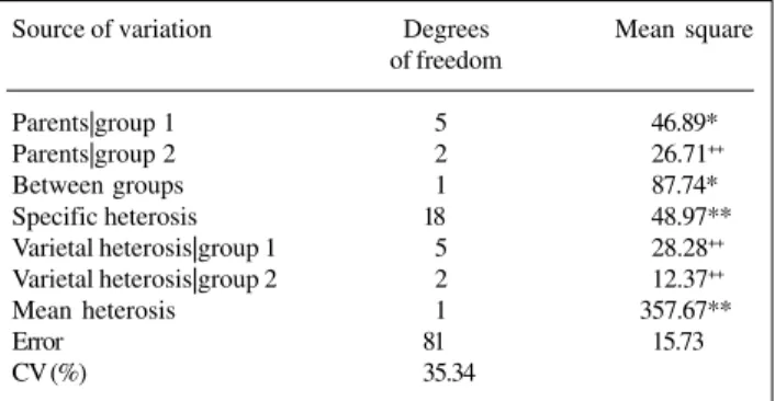
diallel. Table III shows a summary of analysis of variance of parents and their F

1 hybrids, containing only mean

squares supplying informative and non-repetitive tests. Table IV shows the estimates of specific, varietal and mean heteroses. Variance analysis shows presence of genetic variability among parents in group 1. The evidence that the genes determining grain yield are fixed in group 2 is not consistent with results of the diallel analysis considering the additive-dominance model. When there is no genetic variability in one or both groups of parents (wa = 1 and, or,

wa = 1), no relationship exists between covariance and

variance in the arrays, as V(Fr) and/or V(Fs) are equal to

zero. However, analysis of adequacy of the additive-domi-nant model shows a functional relation between W and V (Viana et al., 1999).

The parents in group 2 should not have the same geno-type, for genes determining grain yield. Magnitudes of their observed means (6.10, 4.48 and 9.54, for BAT-304, FT-84-835 and Batatinha, respectively), specific and vari-etal heteroses show differences. Evidence of absence of variability in group 2 must stem from high experimental error, revealed by high magnitude of the coefficient of variation. Accentuated variation among treatment

replica-tions results from the presence, in the same plot, of many-poded plants with well-developed seeds together with plants with few pods with well-formed seeds and several pods without seeds or with undeveloped seeds. This, most probably, owes to low daytime temperatures observed dur-ing plant development. Due to large experimental error, grain yield of the parents in group 2 will be considered different, with approximately 0.19 probability.

Variance analysis indicates, furthermore, that genes determining grain yield are not equally frequent in the two parent groups. Estimate of contrast mL0 - mL0 (3.32)

re-veals that genes increasing grain yield are more frequent in group 1. Tests of hypothesis for specific and mean het-eroses show, as expected, dominance in the polygenic sys-tem determining grain yield. Estimate of mean heterosis shows that dominance effects are predominantly positive, contributing to trait expression increase. The tests of va-rietal heteroses equality show that, in each parent group, allelic genes are equally frequent. However, their differ-ent magnitudes in group 1 and the high experimdiffer-ental error demonstrate that varietal heteroses in this group are not a constant, indicating that the allelic genes are not equally frequent in group 2. When the hypothesis of equality of H0(4): 1

nn’ ∑

n r = 1 ∑

n’ s = 1

trs - 1

2n ∑

n r = 1

tr - 1

2n’ ∑

n’ s = 1

ts ’= 0

Table IV - Estimates of specific (central values), varietal in group 1 (vertical marginal values), varietal in group 2 (horizontal marginal values)

and mean (lower right hand side) heteroses, for grain yield of common beans, in grams, and significance levels for tests of the

hypotheses H0 : hrs= 0, H0 : hr = 0 and H0 : hs = 01.

Parent BAT-304 FT-84-835 Batatinha

Ricopardo 896 4.87++ _1.17++ _{14.34** 6.79*}

Ouro Negro 4.64++ _{10.64* 14.01** 9.76**}

Antioquia 8 15.06** 17.64** 6.28++ _12.99**

DOR. 241 -4.06++ _1.14++ _8.15+ _1.74++

RAB 94 9.81* 6.82++ _0.98++ _5.87+

Ouro 3.67++ _{12.12* 17.37** 11.05**}

5.66* 8.25** 10.19** 8.04

1_{Using the F-statistic. **P < 0.01. *0.01 < P < 0.05.} +_{0.05 < P < 0.10.} ++_{P > 0.10.}

Table III - Summary of the analysis of variance of partial diallel including nine lines of common beans and their F₁ hybrids, for grain yield, in grams.

Source of variation Degrees Mean square of freedom

Parents|group 1 5 46.89*

Parents|group 2 2 26.71++

Between groups 1 87.74*

Specific heterosis 18 48.97**

Varietal heterosis|group 1 5 28.28++

Varietal heterosis|group 2 2 12.37++

Mean heterosis 1 357.67**

Error 81 15.73

CV (%) 35.34

**P < 0.01. *0.01 < P < 0.05. ++_{P > 0.10.}

E(SS(H0(4))) =

(1/4)h2

1 bnn’

1 4bn

1 4bn’)

( + +

σ2₊ ,

E(SS(H0(4))) =

(1/16)h2

1 bnn’

1 4bn

1 4bn’)

( + +

σ2₊ ,

SS(H0(4)) =

2

’2

’ [y..- 1 (y. + y.)]2

2 ’

1 bnn’

1 4bn

1 4bn’)

( + +

varietal heterosis in group 1 is rejected, probability of a type I error is approximately 0.12. It may be considered, therefore, that in group 1, contrary to what happens in group 2, allelic genes affecting grain yield are equally fre-quent.

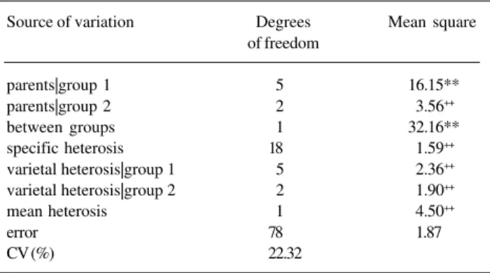
Table V is a summary of variance analysis of the

partial diallel considering data from parents and F2

gen-erations. Results indicate, as expected, genetic variabil-ity in group 1. In group 2 genetic variation is nil or re-duced (P = 0.15), indicating that allelic frequencies in the polygenic system defined by the parents in this group are close to 1 and 0. Estimate of the difference between the means of the two groups (2.00) reveals that genes increasing grain yield occur in greater frequency in group 1. Analysis of dominance in the polygenic sys-tem indicates irrelevance of such genic effects. There-fore, one generation of self-pollination sufficed to markedly reduce the contribution of dominance effects for grain yield. Heterosis manifested in the hybrids is

nil or negligible in the F2 generations. These results

agree with those from the diallel analysis (Viana et al.,

in press).

RESUMO

Com base no trabalho de Hayman de 1954, este artigo discute a análise de variância de tabelas de dialelos parciais. Em razão de muitos dos testes proporcionarem as mesmas inferências, os principais objetivos da análise apresentada são a avaliação da variabilidade genética nos dois grupos de pais e o estudo das het-eroses específica, varietal e média. Testar a nulidade das hethet-eroses específicas é testar a hipótese de ausência de dominância. O teste de igualdade das heteroses varietais em relação aos pais de um grupo é o teste de igualdade das freqüências alélicas no outro grupo. A rejeição da hipótese de nulidade da heterose média indica que há dominância. As informações geradas complementam as resultantes da análise dialélica, envolvendo os genitores e seus híbridos F1 ou

suas gerações F2. Um exemplo com feijoeiro comum é incluído.

REFERENCES

Gardner, C.O. and Eberhart, S.A. (1966). Analysis and interpretation of the variety cross diallel and related populations. Biometrics 22: 439-452.

Geraldi, I.O. and Miranda Filho, J.B. de (1988). Adapted models for the analysis of combining ability of varieties in partial diallel crosses. Rev. Bras. Genet. 11: 419-430.

Graybill, F.A. (1976). Theory and Application of the Linear Model. Duxbury Press, North Scituate, Massachusetts.

Griffing, B. (1956). Concept of general and specific combining ability in relation to diallel crossing system. Aust. J. Biol. Sci. 9: 463-493.

Hayman, B.I. (1954a). The analysis of variance of diallel tables. Biometrics 10: 235-244.

Hayman, B.I. (1954b). The theory and analysis of diallel crosses. Genetics 19: 789-809.

Hayman, B.I. (1958). The theory and analysis of diallel crosses. II. Genetics 43: 63-85.

Jinks, J.L. and Hayman, B.I. (1953). The analysis of diallel crosses. Maize Genet. Cooperation NewsL. 27: 48-54.

Mather, K. and Jinks, J.L. (1974). Biometrical Genetics. 2nd edn. Cornell University Press, Ithaca, New York.

Miranda-Filho, J.B. de and Geraldi, I.O. (1984). An adapted model for the analysis of partial diallel crosses. Rev. Bras. Genet. VII: 677-688.

Searle, S.R. (1971). Linear Models. John Wiley and Sons, New York.

Viana, J.M.S., Cruz, C.D. and Cardoso, A.A. (1999). Theory and analysis of partial diallel crosses. Genet. Mol. Biol. 22: 591-599.

Viana, J.M.S., Cruz, C.D. and Cardoso, A.A. Theory and analysis of partial diallel crosses. Parents and F₂ generations. Bragantia (in press).

(Received May 24, 1999)

Table V - Summary of the analysis of variance of the partial diallel including nine lines of common beans

and their F₂ generations, for grain yield, in grams. Source of variation Degrees Mean square

of freedom

parents|group 1 5 16.15**

parents|group 2 2 3.56++

between groups 1 32.16**

specific heterosis 18 1.59++

varietal heterosis|group 1 5 2.36++

varietal heterosis|group 2 2 1.90++

mean heterosis 1 4.50++

error 78 1.87

CV (%) 22.32