DEPARTAMENTO DE BIOLOGIA VEGETAL
GENERATION AND RECONSTRUCTION
OF EXPERIMENTAL PHYLOGENIES
Tese orientada por Professor Doutor Rogério Tenreiro
Professor Doutor Pedro Silva
ANA MARGARIDA DOMINGOS TAVARES DE SOUSA
Doutoramento em Biologia
(Biologia Molecular)
Acknowledgments
I would like to thank my supervisor, Prof. Rogério Tenreiro, for receiving me in his laboratory and for his guidance. I also thank to my supervisor, Prof. Pedro Silva, for his idea for the theme of this dissertation.
I thank all my colleagues and friends from the laboratory for their help and friendship.
I acknowledge the financial support from Fundação para a Ciência e Tecnologia, which make this work possible (grant PRAXIS XXI/BD/19793/99). I thank my parents, brother, son and Ricardo for all the love, encouragement and support through these years.
Geração e reconstrução de filogenias experimentais
Resumo
A inferência filogenética envolve uma tentativa de estimar a história evolutiva de um conjunto de organismos (taxa) ou de uma família de genes. Isto é equivalente a inferir a sequência de ramificações ou transformações evolutivas que tiveram lugar. Uma forma natural de ilustrar esta questão é através de uma árvore. O padrão de ramificação da árvore (a sua topologia) indica de que forma os taxa estão relacionados, i. e. quais os taxa que partilham o ancestral comum mais recente. Os comprimentos dos ramos, se estiverem incluídos, representam o tempo ou a quantidade de evolução que ocorreu entre cada dois nós na árvore.
O papel tradicional da inferência filogenética tem sido na sistemática biológica, contudo, hoje em dia, constitui uma ferramenta essencial em áreas que vão desde as ciências forenses à previsão da evolução de vírus, das funções de genes não caracterizados e de proteínas ancestrais.
Até hoje não se conhece nenhum algoritmo para inferir árvores evolutivas suficientemente versátil ao ponto de ser adequado a todos os tipos de dados. Em contrapartida, existe uma vasta gama de métodos filogenéticos complementares comummente utilizados, cada um deles com as suas vantagens (e desvantagens) particulares. O trabalho aqui apresentado pretende contribuir para a compreensão destas diferenças fornecendo um “case study” simples e conhecido à partida. Uma das formas de avaliar estas diferenças é através da medição da exactidão da inferência filogenética de cada algoritmo. A avaliação implica um conhecimento antecipado da filogenia verdadeira subjacente a um determinado grupo de taxa. No entanto, na maioria das situações, essa informação não está disponível de forma que este resultado é obtido por estudos de congruência (com base na ideia de que se conjuntos de dados diferentes produzem a mesma árvore então o método é exacto), simulação ou filogenias conhecidas. Os estudos de simulação são insubstituíveis na exploração exaustiva dos efeitos dos modelos de evolução, das topologias das árvores, das taxas de evolução relativas ou absolutas ou de qualquer outro parâmetro que possa afectar a “performance” dos métodos
filogenéticos. Embora estes estudos sejam simplificações grosseiras do processo evolutivo, eles são úteis para detectar generalizações acerca do desempenho dos métodos que possam ser aplicadas a situações reais. As filogenias experimentais permitem testar eficientemente estas previsões. Idealmente o sistema experimental deverá incluir um organismo de crescimento rápido, com genoma de pequena dimensão e capacidade de originar mutantes ao longo de múltiplas gerações de crescimento controlado. Os bacteriófagos parecem corresponder de forma excepcional a estes requisitos, uma vez que podem ser facilmente manipulados em laboratório durante milhares de gerações por ano, possuem genomas de pequenas dimensões e a sua taxa de mutação pode ser facilmente aumentada pela utilização de agentes mutagénicos.
Esta dissertação teve por objectivo principal testar a eficiência de diferentes métodos de inferência filogenética na recuperação da árvore verdadeira numa situação desfavorável para a generalidade dos algoritmos como é o caso de uma topologia assimétrica. Esta árvore compreende a maioria das situações problemáticas previstas pelos estudos de simulação tais como ramos internos curtos, ramos longos e curtos alternados (diferentes taxas de evolução entre os taxa) e ainda a complexidade inerente a um organismo real. Estudos anteriores testaram um sistema equivalente com base numa filogenia completamente simétrica. Esse sistema, considerado pelos autores como um modelo nulo, ou seja a situação mais favorável do ponto de vista da inferência, permitiu validar a potencialidade do sistema (como modelo experimental para estudos filogenéticos) mas não a diferenciação dos algoritmos testados, uma vez que todos inferiram a árvore verdadeira.
Foi testada a possibilidade da utilização de um sistema experimental alternativo para a obtenção de filogenias experimentais. Esse sistema envolveu o fago bIL170, cujo hospedeiro é a bactéria Lactocococcus lactis. Inicialmente tido como um sistema promissor e inovador devido ao seu impacto na indústria de lacticínios, este fago revelou uma fidelidade do complexo de replicação inesperadamente alta, o que impossibilitou a sua utilização como modelo experimental.
O protocolo experimental utilizado para a obtenção da filogenia experimental consistiu na propagação seriada do bacteriófago T7 (cujo hospedeiro é a bactéria Escherichia coli) na presença do mutagénio N-metil-N’-nitro-N’-nitrosoguanidina. Para tal procedeu-se à propagação seriada do fago em meio
líquido, em que cada nova cultura de E. coli era infectada com uma alíquota do lisado anterior. De cinco em cinco lisados este processo era interrompido por um plaqueamento em meio sólido, uma vez que a ocorrência de “bottlenecks” frequentes ajuda à fixação de mutações. Este procedimento foi repetido o número de vezes indicado pelo comprimento dos ramos da árvore representada na Figura 1 do capítulo 3, sendo as bifurcações criadas pela utilização de um stock clonal recuperado de uma única placa fágica para a infecção de duas linhas independentes. Os dados utilizados na inferência filogenética foram de dois tipos: locais de restrição e sequências nucleotídicas. Para tal construíram-se mapas físicos com 36 enzimas para todos os nós (internos e externos) e sequenciou-se 12% do genoma (contidos em 9 regiões diferentes distribuídas ao longo do genoma) de cada um dos fagos correspondentes aos nós terminais.
Quando estão em consideração conjuntos diferentes de dados, que dizem respeito a grande parte do genoma ou a múltiplos genes, é necessária uma análise de congruência. A existência de incongruência ligeira entre os vários conjuntos de dados pode ser devida a amostras de tamanho inadequado, mas a ocorrência de uma forte incongruência pode ter origem em diferentes taxas de evolução entre as partições consideradas (posição no codão, constrangimentos funcionais) ou em partições que tiveram diferentes histórias (transferência horizontal ou duplicação de genes). Por este motivo a análise filogenética foi precedida de uma análise de congruência. Testou-se a congruência entre os dados de restrição e os de sequência, entre os locais de reconhecimento da enzima Sau3AI (enzima cujos locais de reconhecimento no genoma sofreram uma taxa de evolução particularmente alta face às restantes) e os de todas as outras enzimas e ainda entre cada par de genes. Tal como esperado, uma vez que a filogenia verdadeira é conhecida e todas as partições tiveram a mesma história, o número detectado de casos de incongruência grave foi muito reduzido. De facto, o único caso relevante foi a incongruência detectada entre os locais de restrição da enzima Sau3AI e os de todas as outras enzimas. Este resultado, apoiado pela diminuição da precisão da filogenia obtida quando se combinou estas duas partições numa só análise, está em concordância com a hipótese da necessidade de utilização de um modelo de evolução específico para esta enzima.
Os métodos tradicionais de inferência filogenética avaliados foram: “unweighted pair-group method of arithmetic averages” (UPGMA), “neighbour joining” (NJ), evolução mínima (ME), método de Cavalli-Sforza (uLS), método
de Fitch-Margoliash (wLS), máxima parcimónia (MP) e máxima verosimilhança (ML). Além destes foram ainda testados métodos Bayesianos, métodos baseados na compatibilidade e no caso dos métodos de distância, foi ainda calculada a distância Euclidiana com base na frequência de sequências assinatura.
No geral, os dados de restrição produziram estimativas mais precisas, em relação à topologia, do que os dados de sequência. Este resultado pode ser explicado pelo facto dos dados de restrição representarem mais amplamente o genoma e por isso estarem menos sujeitos à violação do pressuposto de independência de evolução entre posições e sofrerem menos os efeitos do enviesamento provocado pelos erros de amostragem. Desta forma não é de estranhar que a combinação dos dados de restrição e dos dados de sequência numa análise única tenha aumentado a precisão da inferência filogenética na maioria dos casos.
A análise do potencial de cada gene para conduzir à inferência da árvore correcta revelou uma forte dependência entre a exactidão da inferência e o tamanho do gene. Por outro lado, a tentativa do estabelecimento de uma relação entre este potencial e a função individual de cada gene não foi conclusiva.
Uma propriedade que torna uma topologia difícil de inferir é a existência de ramos internos curtos, daí que ramos com estas características estejam presentes na árvore planeada. Os resultados obtidos (mesmo no melhor cenário da análise global) revelaram ser estes ramos a principal fonte de erro para os métodos testados. Particularmente dois dos ramos foram incorrectamente inferidos, consistentemente, por todos os métodos excepto aqueles que assumem um relógio molecular (UPGMA, ME e ML com relógio molecular) ou que utilizam a distância baseada em sequências assinatura. A observação de que o número de diferenças de locais de restrição em um destes ramos era bastante inferior ao esperado, tendo em conta o seu comprimento, conduziu a uma experiência de “bootstrap” paramétrico. Nesta experiência os parâmetros do modelo evolutivo foram estimados a partir dos dados reais e a topologia seguida foi equivalente à planeada, excepto no ramo que aparentemente sofreu menos evolução que o esperado (foi-lhe atribuída uma dimensão proporcional ao número de mudanças de locais de restrição). Os resultados da simulação apresentaram uma concordância razoável com os dados reais, excepto no ramo 9-10 (Figura 1, Capítulo 3), que embora erradamente inferido pelos dados reais, não ofereceu problemas
ao estudo de simulação. Posteriormente, métodos de compatibilidade permitiram verificar que também este ramo teve uma quantidade de evolução inferior ao esperado.
Outro dos aspectos a salientar foi o excelente desempenho da distância baseada nas sequências assinatura (particularmente na análise global). Tal como referido anteriormente, apenas este método e os que assumem um relógio molecular conseguiram obter a árvore verdadeira. Uma das hipóteses explicativas para este facto reside na possibilidade do “bias” mutacional deste sistema influenciar as frequências dos motivos de sequências e este facto reflectir-se nas matrizes de distância Euclidiana. Existem outros sistemas com espectros mutacionais semelhantes, tais como os pseudogenes de eucariotas e o vírus HIV; estudos preliminares sugeriram que esta poderá ser igualmente uma boa abordagem para estes casos.
Esta tese tem a seguinte estrutura:
Capítulo 1 – Introduction – apresenta uma introdução à inferência filogenética e aos principais métodos utilizados por esta disciplina. Faz uma revisão bibliográfica dos principais trabalhos publicados relacionados com filogenias experimentais. Descreve sumariamente os modelos experimentais utilizados. Capítulo 2 - Experimental phylogenies: picking a (the right) model – Demonstra os passos necessários à selecção de um modelo adequado à construção de filogenias experimentais tomando como exemplo o fago bIL170.
Capítulo 3 – Exploring tree-building methods and distinct molecular data to
recover a known asymmetric phage phylogeny – Apresenta a construção de
uma filogenia experimental (utilizando o fago T7) e sua utilização na comparação da eficácia de métodos tradicionais de inferência filogenética com outros mais recentes ou em estado primordial. Apresenta ainda uma análise comparativa de vários tipos de dados.
Capítulo 4 - Inference of an experimental phage phylogeny with compatibility
methods: comparison with parsimony – Discute a importância da homoplasia
na inferência filogenética e a eficácia de métodos desenvolvidos para obviar os seus efeitos.
Capítulo 5 – Concluding remarks – Comenta as principais conclusões deste trabalho e discute futuros desenvolvimentos.
Palavras-chave: Métodos de inferência filogenética, filogenias experimentais, modelos experimentais, bacteriófago T7, evolução molecular.
Abstract
Experimental phylogenies built through controlled laboratory evolution of actual organisms seem to be an excellent way of testing predictions from simulations. Nevertheless, choosing a model for these studies is not always a straightforward matter. This work presents the steps necessary to select such a model using bacteriophage bIL170 as an example. This phage which seemed a promising and innovating system revealed an unexpected high fidelity replication complex thus impairing its potential as a valuable experimental model.
The construction of an experimental phylogeny with phage T7 is reported. This phage was propagated in the presence of a mutagen following an asymmetric tree topology. The performance of several phylogenetic methods was tested using restriction sites and nucleotide data. Only methods that encompassed a molecular clock or those based on sequence signatures recovered the true phylogeny. The probable explanation for the exceptional performance of the sequence signature based methods lies in the mutation bias of this system which can shift motif frequencies and be reflected in the Euclidean distance matrices. If this hypothesis is confirmed, this methodology may be extended to infer phylogenies within systems with similar mutation spectrums, such as eukaryotic pseudogenes and HIV virus.
All the other methods failed consistently in the inference of two internal branches. To test if these results could have been predicted by simulation studies, a parametric bootstrap experience was conducted using the true tree and the evolution parameters estimated from the real data. The simulation predicted most but not all of the problems encountered by phylogenetic inference methods. Short interior branches may be more prone to error than predicted by theoretical studies.
With the level of homoplasy registered in this study, the performance of compatibility based methods (which allegedly eliminate homoplastic characters from the analysis) could not be distinguished from parsimony.
Keywords: Phylogenetic inference methods, experimental phylogenies, experimental models, bacteriophage T7, molecular evolution.
Contents
Acknowledgements iii
Resumo v
Abstract xi
1 Introduction (Phylogenetic inference) 1
1.1. Philosophical foundation 1
1.2. Applications 2
1.3. Methods 5
1.3.1 Distance matrix methods 6
1.3.1.1 Least squares methods 6
1.3.1.2 Minimum evolution 7
1.3.1.3 Unweighted pair group method with arithmetic mean 7
1.3.1.4 Neighbor-joining 8
1.3.1.5 Distance measures 9
1.3.1.6 Alignment-free sequence comparison (distances) 12
1.3.2 Maximum parsimony methods 14
1.3.3 Maximum likelihood methods 18
1.3.3.1 Models of nucleotide evolution 21
1.3.3.2 Assessing confidence – bootstrap 23
1.3.3.3 Parametric bootstrap 24
1.3.3.4 Molecular clock tests 24
1.3.4 Bayesian methods 25
1.4 Tree disagreement: incongruence and competing trees 28
1.4.1 Incongruence length difference test 28
1.4.2 Sitewise tests 29
1.4.3 Kishino-Hasegawa test 30
1.4.4 Shimodaira-Hasegawa test 32
1.4.5 Swoford-Olsen-Wadel-Hillis test 33
1.5 Assessing phylogenetic accuracy 34
1.5.1 Simulation studies and known phylogenies 35
1.6 Experimental model: bacteriophages 43
1.6.2 Bacteriophage T7 47
1.7 Scope of the thesis 48
1.8 References 49
2 Experimental Phylogenies: picking a (the right) model 61
2.1 Introduction 62
2.2 Materials and Methods 64
2.2.1 Phages, bacterial strains and media 64
2.2.2 Growth studies (for host and phage) in suboptimal conditions 64
2.2.3 Serial propagation of bIL170 in the presence of 0.03 % bile salts 65
2.2.4 Serial propagation of bIL170 in the presence of 250 µg NG ml-1 65
2.2.5 DNA extraction and restriction 66
2.2.6 PCR amplification and sequencing 66
2.2.7 Sequence data analysis 68
2.3 Results 68
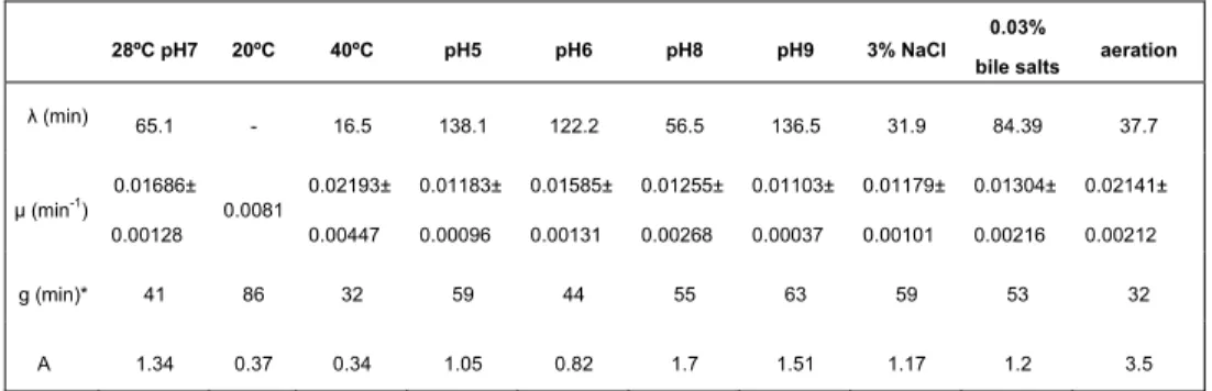
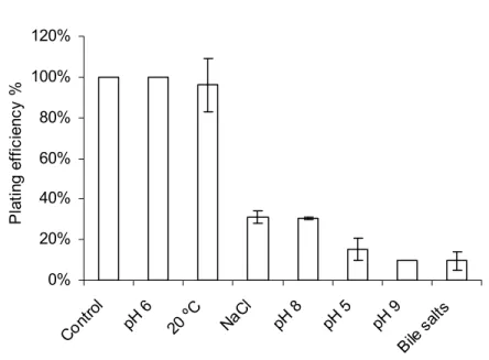
2.3.1 Determination of growth parameters (phage and bacterium) led to the choice of a condition that poses a significant level
of stress to the bacterium- phage system. 68
2.3.2 Serial lysates in the presence of bile salts and restriction
analysis of the phage genome 71
2.3.3 Serial lysates in the presence of NG and sequence analysis 72
of 20 % of the phage genome
2.4 Discussion 73
2.5 Acknowledgements 76
2.6 References 77
3 Exploring tree-building methods and distinct molecular data to
recover a known asymmetric phage phylogeny 81
3.1 Introduction 82
3.2 Materials and Methods 84
3.2.1 Propagation of bacteriophage T7 84
3.2.2 Phylogeny construction 85
3.2.4 Sequence data 86
3.2.5 Phylogenetic analysis 87
3.3 Results and discussion 89
3.3.1 Inferred and actual phylogeny comparison 91
3.4 Conclusions 104
3.6 References 107
4 Inference of a known phage phylogeny with compatibility methods:
comparison with parsimony 113
4.1 Introduction 114
4.2 Materials and Methods 123
4.2.1 Phylogenetic inference 124
4.3 Results and discussion 125
4.6 References 130 5 Concluding remarks 133 5.1 References 136 Annex 1 137 Annex 2 149 Annex 3 155 Annex 4 161 Annex 5 165 Annex 6 173
Chapter 1
Introduction
Phylogenetic inference
“Phylogenies, or evolutionary trees, are the basic structures necessary to think clearly about differences between species, and to analyse those differences statistically. They have been around for over 140 years, but statistical, computational, and algorithmic work on them is barely 40 years old.” [1]
1.1 Philosophical foundation
The biological process of evolution – descent with modification – generates and structures the remarkable diversity of life on Earth today and in the geological past [2]. Continued speciation generates groups of related species that can be represented by a unique inclusively hierarchical pattern of relationships between all organisms based on their similarities and differences which Darwin named “Tree of life” [3]. Even now, the meaning, role in biology, and support in evidence of the universal Tree of life, is still in debate. The central metaphor of phylogenetics is the Tree of life and imagination of its unity and uniqueness is of philosophical nature [4]. Many evolutionists believe that we have already, or will in time, reconstruct this tree quite accurately. Other evolutionists question even this most fundamental belief, that there is a single tree [5]. They argue that lateral gene transfer, recombination, gene loss, duplication, and gene creation are a few of the processes that cause variation
within and between bacterial species that is not due to vertical transfer. Therefore the Tree of life is not a useful way of modelling life at this level [5].
The second half of the 20th century witnessed the growth of a great interest in
phylogenetic reconstructions at macrotaxonomic level [6]. This was not a revival of classical phylogenies, rather a new approach emerged as a result of the merging of three disciplines, namely cladistics, numerical phyletics and molecular phylogenetics [6]. Thus, the new phylogenetics could be defined as a branch of evolutionary biology aimed at elaboration of “parsimonious” cladistic hypotheses by means of numerical methods on the basis of mostly molecular data. The main input of molecular phylogenetics was due to molecular data which makes it possible to compare directly such far distant taxa as prokaryotes and higher eukaryotes. Also the development of algorithm methods (numerical phylogenies) was only possible once computers were available [1].
1.2 Applications
Reconstruction of the evolutionary history of genes and species was the first role of phylogenetic inference methods. Only the production of reliable phylogenies can help to understand the sequence of evolutionary events that generated present day diversity and the mechanisms of evolution. In the present, however, there is also a growing recognition of trees as a tool for understanding biological processes not necessarily related to phylogenetics or to evolution per se. The following works, summarily described, aim to reflect this fact.
Finding residues that are important to natural selection might help to predict the evolution of influenza virus and assist vaccine preparation.
In 1999, Bush et al. [7,8] found eighteen codons in the HA1 domain of the hemagglutinin genes of human influenza A virus that appear to be under
positive selection1. They thought that if the selective pressure was to evade
the host immune system, then virus sustaining mutations at these codons in
1 Positive selection is defined as a significant excess of nucleotide substitutions that result in
the past should have been more fit2 than other coexisting virus. In addition, if
this hypothesis was correct, then screening extant strains for additional mutations in these codons might help to identify the most fit viral strains in circulation. The construction of (most parsimonious) phylogenetic trees using hemagglutinin genes revealed, over time, a single successful lineage, which they called “trunk lineage”. The trunk lineage is the only lineage from which strains in all subsequent years arise and its course within the upper portions of the tree (most recent influenza season) becomes identifiable only in retrospect. So they performed retrospective tests for 11 influenza seasons and searched for the lineage undergoing the most amino acid replacements in the 18 positively selected codons in every season. These lineages identified the section of the tree from which the future lineage emerged in 9 of the 11 seasons tested. They claimed that these methods can be used to examine the evolution of the hemaggluitinins of influenza B and influenza A H1 viruses circulating in humans to identify sets of codons that may have predictive value for these important pathogens. It has also been argued that this information might assist vaccine preparation [9].
Predicting function of uncharacterized genes
In the genomic age, in which numerous gene sequences are generated with little or no accompanying experimentally determined functional information, the ability to accurately predict gene function based on gene sequence is an important tool. Eisen [10,11] noted that almost all functional prediction methods rely on the identification, characterization, and quantification of sequence similarity between the gene of interest and genes for which functional information is available. However since sequence similarity does not ensure identical functions, the same author suggested that functional predictions could be greatly improved by focusing on how genes became similar in sequence (by phylogenetic analysis) rather than on the sequence similarity itself. He identified several conditions in which similarity methods produce inaccurate predictions of function and proposed a method that makes use of information about evolutionary relationships among genes to predict the functions of uncharacterized genes. Such unfavourable conditions include: functional change during evolution, functional change and rate variation, and gene duplication and rate variation. He claims that phylogenetic methods have
2 The viral strain most closely related to future lineages was considered the best fit strain
the advantage, over similarity methods, of correcting for most of this problems by the process of masking (exclusion of regions of genes in which sequence similarity is misleading rather than biologically important) and by the allowance for evolutionary branches to have different lengths. The method to predict the functions of uncharacterized genes involves: a) the identification of homologous genes to the gene of interest, b) aligning sequences, c) building phylogenetic tree, d) overlaying known functions onto tree and finally e) infer likely function of gene of interest (uncharacterized genes can be assigned a
likely function if the function of any ortholog3 is known).
Inference of ancestral proteins
In 1963 Pauling and Zukerkandl [12] first suggested the use of phylogenetic inference in predicting ancestral sequences. Since then, this technique has been used to predict primary structures of ancient proteins, and the function of these proteins has been tested following expression of the recreated gene. An interesting example of these studies was presented by Wouters et al. [13] who recreated an ancestor to one of the subbranches of the trypsin superfamily of serine proteases. In this superfamily, non trypsin-like primary specificities have arisen in only two monophyletic descendent subbranches. They reconstructed an ancestral to one of these non-trypsin members by total gene synthesis and protein expression. Ancestral sequence prediction was made using parsimony (a maximum-likelihood tree was also constructed and found to exhibit a high level of congruence to the maximum parsimony tree). Unlike the extant members of this serine protease family, the recreated ancestor tolerates mutational changes in the specificity conferring residues. However, the cost of this “structural and functional plasticity” is a relaxation of the presumed narrow trypsin-like primary specificity of its immediate predecessor. That is, despecialization or evolution in reverse was required for further diversification. Functional studies of the reconstructed enzyme indicate that this deep evolutionary reconstruction (<170 million years old) is accurate. Such remarkable reconstruction was only possible because of phylogenetic inference methods.
3 Homologous genes (genes descended from a common ancestor) that have diverged from each
Forensic science
A paradigmatic example of phylogenetic inference application in forensic science is the Florida dental case. In 1992, Ou et al. [14] reported a case of a Florida dentist suspected of transmitting human immunodeficiency virus (HIV) to some of his patients. It is known that for a virus with substantial genomic variation (such as HIV), identification of strains with a high degree of genetic relatedness may imply an epidemiologic linkage between persons infected with these strains. They sequenced the C2-V3 domains of the gp120 gene of HIV obtained from the dentist, seven patients and 35 control individuals from the local population. Phylogenetic analyses of these sequences originated many equally parsimonious trees; however, the monophyletic clade containing the sequences of the dentist and five of the patients (the dental clade) was common to all of the trees. The other two patients had already been confirmed to have other risk factors for HIV infection. To assess the reliability of the inferred dental clade, later Hillis et al. [15], noticing an important departure in HIV evolution from the Kimura model of evolution (see section 3.2.2.3), took the relative frequencies of all 12 types of nucleotide change and the estimated phylogeny as a model to simulate the phylogeny at varying rates of overall change. They concluded that at the level of change seen in the original study, 90% to 94% of all the branches in the tree were resolved in the simulations by every method except UPGMA, and that the dental clade was resolved 100% of the time with every method except UPGMA. They added that these simulations results provided significant support for a phylogeny consistent with the dental transmission hypothesis, although they acknowledge that no simulation can take all the complexities of HIV evolution into account. For example changes in HIV that result from the duration of the infection, pressure from the host’s immune system, stage of the disease or therapy can result in parallel evolution across lineages and reduce the probability of correct estimation.
1.3 Methods
There are an ever growing number of methods for molecular phylogenetic inference. These methods differ essentially by how they handle the data and by the approach taken when building trees. The next section will describe some of the most used and well known methods.
“Proceeding from the simple assumption that as the time increases since two sequences diverged from their last common ancestor, so does the number of differences between them, tree estimation seems to be a relatively simple exercise: count the number of differences between sequences and group those that are most similar. The simplicity of such an algorithm underestimates the complexity of the phylogenetic-inference problem. The rate of sequence evolution is not constant over time, so a simple measure of the genetic differences between sequences is not necessarily a reliable indication of when they diverged. Natural selection or changing mutational biases during the history of an organism might cause distantly related sequences to diverge from each other more slowly than is expected, or even become more similar to each other at some residues. Many of the sites in a DNA sequence are not helpful for phylogenetic reconstruction: some are functionally constrained so that they are invariant among all known sequences; others evolve rapidly (and, therefore, are not reliable indicators of deep relationships). As a result of such ‘noise’, often several phylogenetic hypotheses can explain the data reasonably well. So, the researcher must take this uncertainty into account.” [9]
1.3.1 Distance matrix methods
Distance matrix methods comprise a large family of methods first introduced by Cavalli-Sforza and Edwards (1967) [16] and by Fitch and Margoliash (1967)
[17]. They assume that a measure of the distance4 between each pair of taxa
is calculated and then find a tree that predicts the observed set of distances as accurately as possible. Computer simulations have shown that the amount of information that is lost by transforming sequences into a table of pairwise distances is remarkably small [1].
In distance matrix methods, branch lengths are not simply a function of time,
they reflect expected amounts of evolution in different branches of the tree
.
1.3.1.1 Least squares methods
The basis of distance matrix methods is to construct a matrix of observed
distances (Dij) from the data and then infer a tree which branch lengths
4 The evolutionary distance is defined as the number of base substitutions per homologous site
represent the predicted distances (dij). Least squares methods measure the
discrepancy between observed and predicted distances:
=
Q
∑
∑
(
)
= =−
n j ij ij ij n id
D
w
1 2 1(1)
wij represents weights that differ between different least squares methods.
Cavalli-Sforza and Edwards (1967) [16] defined the unweighted least squares
method in which wij = 1 and Fitch and Margoliash (1967) [17] used wij = 1/Dij5.
The tree topology and branch lengths that minimize Q are chosen.
1.3.1.2 Minimum evolution (ME)
The minimum evolution method as presently used was introduced by Rzhetsky and Nei [18,19]. The criterion used by this method to choose the best tree is to minimize total branch length (S). In the ME method the tree is fitted to the data and the unweighted least squares method is used to determine the branch lengths. The shortest total length least square tree is chosen among every possible topology.
1.3.1.3 Unweighted pair group method with arithmetic mean (UPGMA)
Unweighted pair group method with arithmetic mean [20] instead of choosing the best tree by some criterion from all the possible trees is an algorithm that builds the tree directly from the distance matrix (clustering algorithm). UPGMA assumes that the evolutionary rate is the same in al lineages (a molecular clock is in effect). This amounts to constrain the branch lengths in a way that the distance from the root to any tip is the same. Beginning with the distance matrix the algorithm works in the following way [1]:
1. It finds the pair of taxa, i and j that have the smallest distance, Dij.
2. Creates a new group, (ij), which has n(ij) = ni + nj members.
3. Connects i and j on the tree to a new node. The two branches
leading to i and j each have a length of Dij / 2.
5 See chapter 3 for an application of these two methods named as weighted and unweighted least
4. Computes the distance between the new group and all the other groups by using: jk j i i ik j i i k ij
D
n
n
n
D
n
n
n
D
⎟
⎟
⎠
⎞
⎜
⎜
⎝
⎛
+
+
⎟
⎟
⎠
⎞
⎜
⎜
⎝
⎛
+
=
), ((2)
5. Deletes the columns and rows of the data matrix that correspond to groups i and j, and adds a column and row for group (ij).
6. Return to step 1.
The main disadvantage of UPGMA is that it can lead to seriously wrong trees if the distance matrix reflects a substantially nonclocklike tree. For instance if the evolutionary rate is not the same on different branches, two distant taxa may be joined simply because they are similar in not having changed.
1.3.1.4 Neighbor-joining (NJ)
Neighbor-joining [21] is also a clustering algorithm, it approximates a simplified version of the ME method for inferring a bifurcating tree [22]. In this method, the S value is not computed for all the topologies but the examination of different topologies is imbedded in the algorithm, so that only one final tree is produced. It starts with a star phylogeny in which all interior branch lengths are
zero. The total branch length of this topology (S0) is clearly much higher than S
for the true tree. The next step is to compute Sij for a tree in which i and j are
neighbors (connected through a single interior node) and separated from the rest of the taxa. As it is impossible to know a priori which pair of neighbors minimize S, this procedure must be repeated with every pair of taxa to choose
the one that produces the tree with the smallest Sij. This pair of taxa is then
regarded as a single taxon, and the next pair of taxa that gives the smallest sum of branch lengths is again chosen. This process is continued until all multifurcating nodes are resolved into bifurcating ones.
When the extent of sequence differences and the number of nucleotides examined are sufficiently large, NJ nearly always produces the same topology as ME [23,24]. However when the sequence length is <500 bp NJ tree can be considerably different from ME tree, even though the difference in S is usually statistically nonsignificant [19].
When variation of evolutionary rates from site to site is large, correction of distances become increasingly important. While likelihood methods can use information from changes in one part of the tree to inform the correction in others, distance matrix methods are inherently incapable of propagating information in this manner [1]. This constitutes a disadvantage of these methods.
1.3.1.5 Distance measures
The evolutionary distance between a pair of sequences is usually measured by the number of nucleotide or amino acid substitutions between them. Theoretically, if the total number of substitutions between any pair of sequences is known, all the above described distance methods (except for UPGMA with non ultrametric numbers of susbstitutions) produce the correct phylogenetic tree [22]. However, this number is almost always unknown and since the most serious problem of distance methods is that they require a reliable measure of evolutionary distances between sequences, many different methods (evolutionary models) for estimating this number have been proposed. Some of these methods may be very sophisticated and include several parameters. The most common parameters are added to correct for the different substitution rates for each type of nucleotide change, for the proportion of sites which are unable to change and for variable rates across sites and among lineages. Combining different parameters has resulted in a large number of models [25] and a corresponding number of evolutionary distances. Nevertheless in this section only those distances used in chapter 3 will be described (see section 1.3.3.1 for more information on evolutionary models). The efficiency of distance measures in obtaining the correct tree depends on at least two factors: the linear relationship with the number of substitutions and the standard error or coefficient of variation of the estimate of the distance measure [22].
p - distance
This distance is merely the proportion (p) of nucleotide sites at which the two sequences compared are different. This is obtained by dividing the number of
n
n
p
=
d(3)
The p-distance is approximately equal to the number of substitutions per site only when p is small (<0.1). The computation of this distance is simple and it gives essentially the same results as more complicated distances as long as all pairwise distances are small [26].
Jukes-Cantor (JC) distance
The Jukes-Cantor distance [27] is based on the simplest possible model of DNA sequence evolution. It assumes that the four bases have equal frequencies, and that all substitutions are equally likely. Under this model the distance between two sequences is given by:
⎟
⎠
⎞
⎜
⎝
⎛ −
−
=
p
d
xy3
4
1
ln
4
3
(4)
dxy represents the distance between sequence x and sequence y expressed as
the number of nucleotide substitutions per site and p is computed by using equation (4). ln, the natural log function is used to correct for superimposed substitutions. The 3/4 and 4/3 terms reflect that there are four types of nucleotides and three ways in which a second nucleotide may not match a first with all types of change being equally likely (i. e. unrelated sequences should be 25% identical by chance alone).
Kimura’s two parameter (K2P) distance
Kimura’s two parameter model [28] differs from Jukes-Cantor’s because it doesn’t assume that all substitutions have the same probability. K2P incorporate the observation that the rate of transitions (α) per site may differ from the rate of transversions (β) [29]. In this model the number of nucleotide substitutions per site is given by:
(
)
(
)
⎥
⎦
⎤
⎢
⎣
⎡
−
+
⎥
⎦
⎤
⎢
⎣
⎡
−
−
=
Q
Q
P
d
xy2
1
1
ln
4
1
2
1
1
ln
2
1
(5)
where P and Q are the proportional differences between the two sequences due to transitions and transversions, respectively. If α = β, then the K2P model becomes the JC model.
Upholt and Nei-Li distances
Much of the early work on variation in DNA sequences used variation in restriction sites rather than full sequences. The first distance between restriction sites pattern was derived by Upholt [30]. It assumes a Jukes-Cantor model of evolution, that is, all nucleotide sites have an equal probability of undergoing a substitution. Thus the distance between two sequences (x and y) digested with an enzyme r-base cutter with a proportion S of ancestral restriction sites remaining unchanged in both lines is given by:
( )
r
S
d
xy=
−
ln
(6)
Nei and Li [31] developed a similar distance that also assumes a Jukes-Cantor model of base change and that identical sites are those that remain unchanged from the common ancestor. It includes a correction for gamma distribution of rate of change among nucleotide sites.
⎥
⎥
⎦
⎤
⎢
⎢
⎣
⎡
⎟⎟
⎠
⎞
⎜⎜
⎝
⎛
−
⎟
⎠
⎞
⎜
⎝
⎛
−
=
ln
4
1
/
3
2
3
21r xyS
d
(7) In this case,
(
X Y)
XYn
n
n
S
+
=
2
ˆ
(8)
Where nXY is the number of shared restriction sites between the two
sequences X and Y, and nX and nY are number of restriction sites present in
sequences X and Y, respectively.
1.3.1.6 Alignment-free sequence comparison (distances)
It is commonly believed that to infer a phylogenetic tree representing the history of a set of molecular sequences, they need first be arranged relative to each other in a way that represents the best hypothesis of homology at every position; i.e., an optimal multiple sequence alignment [32]. Most alignment methods implicitly make the assumption of collinearity over long stretches
frequently leading to suboptimal alignments in cases of sequences that have
undergone recombination, proteins with shuffled domains, and genomic sequences (which often feature large-scale rearrangements) [33]. Alignment-free methods are devoid of this assumption and have proven to be very useful in a number of these situations [34-37]. Nevertheless the proposition of these methods is recent being the earliest systematic publications from Blaisdell [38]. Two main categories of methods have been proposed – methods based on word frequency, and methods that do not require resolving the sequence with fixed word length segments. They include the use of Kolmogorov complexity theory and scale-independent representation of sequences by iterative maps. This last category will not be further commented since it is still in experimental development, and to our knowledge has not yet been consistently applied to phylogenetics.
Sequence signatures distances
All the distance measures in section 1.3.1.5 require a prior sequence alignment followed by a mismatch count and then the assumption of an evolutionary model (except for p distance) permits the computation of distances themselves. Sequence signatures based distance doesn’t assume such a model. Instead it computes the whole set of frequencies of short oligonucleotides (words, until ten nucleotides [34]) of the sequences and then different types of comparisons based in some distance definitions between frequencies of L-words can be made to construct a distance matrix. The basic rationale for sequence comparison is that similar sequences will share word
composition to some extent, which is then quantified by a variety of techniques [39].
A sequence X, of length n, is defined as a linear succession of n symbols from a finite alphabet, A, of length r.
A segment of L symbols, with L ≤ n, is designated an L-tuple. The set WL
consists of all possible L-tuples that can be extracted from sequence X and has K elements.
{
L L LK}
LW
W
W
W
=
.1,
.2,...,
. Lr
K
=
(9)The identification of L-tuples in the sequence X can then be the object of counting occurrences with overlapping (Equation 10). Computationally, the counting is usually performed by taking a sliding window L-wide that is run through the sequence, from position 1 to n – L + 1.
)
,...,
(
.1 X. K L X L X Lc
c
c
=
(10)
The vector of frequencies
f
LX is obtained as the relative abundance of eachword (Equation 11).
1
1 . 1 . 1 .−
+
=
⇔
=
∑
=n
L
c
f
c
c
f
X L X L K j X j L X L X L(11)
For example, for a sequence A = {ATCG}, r = 4, a three letter word, L = 3, could be w = ATC. For the sequence X = ATATAC, where n = 6, the vector
Y
p
3 is estimated by the relative frequencies of all trinucleotides. Thefrequencies, determined by sliding a three letter window n – L + 1 = 4 times would be:
}
{
,
,
,
,...
3
ATA
TAT
TAC
AAA
W
=
(
2
,
1
,
1
,
1
,
0
,...
)
3=
Xc
(
0
.
5
,
0
.
25
,
0
.
25
,
0
,...
)
3X=
f
The vectors
c
3X andf
3X have length K = 43 = 64 and the zero coordinatescorrespond to missing words in X, in this case absent trinucleotides [39]. Sequence signatures can be easily computed with the algorithm “Chaos game representation” [40]. Species-specificity and conservation of signature in any part of the genome makes sequence-signature a promising tool for phylogenetic analysis [41].
The first distance, between two sequences, computed from L-tuple counts, was the square Euclidean distance [38] (Equation 12).
(
)
∑
(
)
=−
=
K i Y i L X i L E LX
Y
c
c
d
1 2 . .,
(12)
Since then a large variety of metric systems have been proposed, for example the calculation of the linear correlation coefficient from L-tuple frequencies [42], distances that take into account the data covariance structure (Mahalanobis [43] and standardized Euclidean), a pattern-based approach [33,44], and many others.
1.3.2 Maximum parsimony (MP) methods
Maximum parsimony is a family of methods that seek the tree involving the minimum net amount of evolution [45] (compatible with the minimum number of substitutions among sequences [46]). The total number of evolutionary changes in a tree is the sum of the number of changes in each position (tree length). The length of each possible tree is computed and the topology that requires the smallest number of substitutions is chosen to be the best tree [47]. MP is expected to find the correct tree as long as no multiple substitutions occur and a sufficient number of informative nucleotide positions are provided. A position is considered phylogenitically informative only if it favours some trees over the others. This will only happen if a minimum of two different nucleotides exist in that position and each of the character states is represented in at least two of the sequences under study [48].
There are three stages in the construction of the MP tree: the optimality criterion used to infer the tree, the algorithm employed in the search for optimal trees under those conditions and the measure used to evaluate the result. The optimality criterion specifies the restrictions imposed on character
changes, while the algorithm that searches for the optimal tree is concerned with the practical problem of inspecting all possible topologies [49]. There are multiple optimality options, in this work only those concerning nucleotide sequences will be discussed.
Camin and Sokal [50] first proposed a discrete character parsimony analysis. Their method included the restriction that character transformations are
irreversible, that is they assumed evolution to be irreversible. All homoplasy6
must therefore be accounted for by parallelism or convergence. Such a restriction will be unwarranted most of the times, so this condition has since been relaxed.
The Wagner method is appropriate for binary or ordered multistate characters [51,52]. Yet it is unlikely that there would be sufficient knowledge to allow ordering of nucleotide character states.
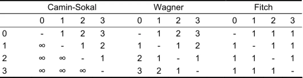
Fitch [47] expanded the original Wagner algorithm to allow for unordered multistate characters, where any state is allowed to transform directly into any other state; that is any nucleotide can transform with equal probability into any of the others. This is the most frequently used initial condition. In fact, all the above parsimony models can be considered special cases of a generalized method of parsimony. Under the generalized parsimony criterion a “cost” is assigned to each transformation between states. The costs are represented as a square m-by-m matrix, in which the elements, Sij, represent the increase in tree length associated with the transformation from state i to j, and m is the total number of states for the character. The stepmatrices for Camin-Sokal, Wagner and Fitch parsimony are represented in Table 1.
Table 1 - Comparison of m x m stepmatrices for Camin-Sokal, Wagner and Fitch parsimony
Camin-Sokal Wagner Fitch
0 1 2 3 0 1 2 3 0 1 2 3 0 - 1 2 3 - 1 2 3 - 1 1 1 1
∞
- 1 2 1 - 1 2 1 - 1 1 2∞ ∞
- 1 2 1 - 1 1 1 - 1 3∞ ∞ ∞
- 3 2 1 - 1 1 1 -6 Homoplasy relates to similarity that arose through convergence or parallel evolution rather then
Weighted parsimony
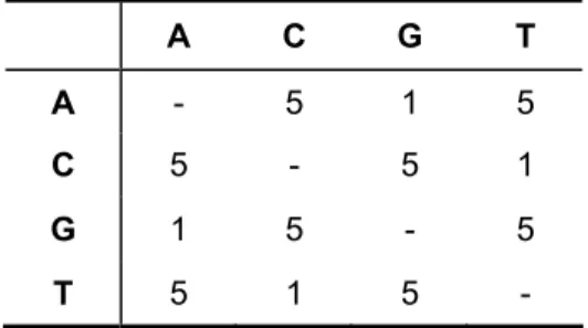
There are two types of a priori weighting fundamentally different; one weights characters and the other weights character state changes [49]. Examples of the first type of weighting is assigning different weights to paired and unpaired sites, where paired sites are those which form Watson-Crick base pairs in the stem regions of a molecule and unpaired sites are those that occur in the loop regions of a molecule. Another example of the same type is the differential weighting of the first, second and third nucleotide positions in codons. “Transversion parsimony” is an example of the second type of weighting. It follows the observation that transversions occur much more rarely than do transitions. Table 2 illustrates a model in which transversions are allocated five times the cost of transitions. Under this model, it would require at least five transition substitutions to support an alternative topology before a topology supported by a single transversion substitution would be rejected.
Table 2 – Stepmatrix for transversion parsimony
A C G T A - 5 1 5 C 5 - 5 1 G 1 5 - 5 T 5 1 5 -
In addition to a priori weighting a posteriori weighting is also possible. Farris [53] suggested a successive weighting algorithm based on the fit of the characters to the tree obtained after a round of analysis with equal weights. These a posteriori weights are then used as input for another (successive) analysis. This procedure can be repeated until the weights or the trees do not change for two consecutive analyses. The idea is to give higher weight to characters consistent with the tree and penalize characters which fit the tree poorly (are homoplastic). Reweighting can be based on the consistency index, retention index or rescaled consistency index (see next section for an explanation of these indexes).
Goodness of fit statistics
There are several parameters that measure the fit of characters to particular
trees [52,54,55]. Three parameters are used to define these indices
.
s = length (number of steps) required by the character on the tree
being evaluated.
m = minimum amount of change that the character may show on any
possible tree.
g = maximum possible amount of change that a character could
possibly require on any conceivable tree.
Overall indexes are calculated for a group of characters by the sum of individual characters parameters:
Consistency index CI =
∑
∑
s
m
Retention index RI =(
(
)
)
∑ ∑
∑ ∑
−
−
m
g
s
g
Rescaled consistency index7 RC = CI . RI
The better the evaluated tree explains the data the closer to 1 these indices will be.
Some properties of parsimony
Felsenstein has deduced under what circumstances parsimony will make a maximum estimate of the tree, that is both maximum parsimony tree and maximum likelihood tree will be the same. These circumstances involve low rates of rates of change even though the different characters may have very different rates of change [56].
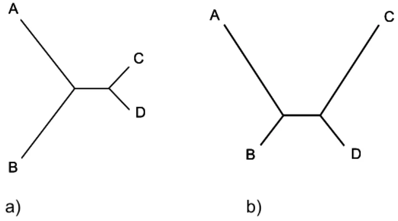
The same author had previously identified the region of the parameter space in which Parsimony will give inconsistent estimates of the tree (Figure 1, b)). This has become known as the “Felsenstein zone” and may be described as the situation where “long branches attract” [57].
Kim [58] examined a number of special cases finding that there were exceptions to many proposed generalizations about when parsimony would be consistent, such as “long branches do not necessarily result in inconsistent estimates if large numbers of data are involved” or “even trees with equal branch lengths can produce inconsistent estimates”.
Felsenstein [59] proposed that imposing a molecular clock was sufficient to assure that parsimony was consistent, yet Hendy and Penny [60] have shown that this may not hold by giving an example that includes internal short
branches8.
Yang [61], Siddall [62], and Steel and Penny [63] have pointed out a region of the tree space in which parsimony outperforms likelihood (Figure 1, a)). This zone has become known as the “Farris zone”. The inherent bias of Parsimony towards long branch attraction helps guarantee that in this situation the tree is correctly inferred.
a) b)
Figure 1 – a) A tree in the Farris zone. b) A tree in the Felsenstein zone.This happens because there is no correction for parallel changes on the two branches, and those changes are reconstructed as occurring on the branch ancestral to the two long branches.
1.3.3 Maximum likelihood (ML) methods
Maximum likelihood methods were first applied to phylogenetics by Edwards and Cavalli-Sforza [64] for gene frequency data. Neyman [65] applied ML estimation to molecular sequences (aminoacids and nucleotides) but it was not
8 The situation posed by these authors might be similar to the one described in Chapter 3.
A B C D A B C D A B C D A B C D A B C D A B C D
until Felsenstein’s implementation [66] that a general ML approach was fully developed for nucleotide sequence data.
The method of ML depends on the complete specification of the data and a probability model to describe the data. The probability of observing the data under the assumed model will change depending on the parameter values of the model. The ML method chooses the value of a parameter that maximizes the probability of observing the data [67].
An example of the computation of the likelihood of tree will be given in order to facilitate the understanding of these methods. For ML methods the data are the individual site patterns. Consider the following aligned DNA sequences of
s = 4 taxa and m sites:
Taxon 1 ACCAGC Taxon 2 AACAGC Taxon 3 AACATT Taxon 4 AACATC
The observations are x1 = {A,A,A,A}’, x2 = {C,A,A,A}’, x3 = {C,C,C,C}’, x4 =
{A,A,A,A}’, x5 = {G,G,T,T}’ and x6 = {C,C,T,C}’. Two of the sites exhibit the
same site pattern (x1 and x4). There is a total of r = 4s site patterns possible for
s species. The number of sites exhibiting different site patterns can also be
considered as the data in a phylogenetic analysis. For example, the above data matrix can also be described as:
Taxon 1 AAAAAAAAA...C...C...C...G...TTT Taxon 2 AAAAAAAAA...A...C...C...G...TTT Taxon 3 AAAACCCCG...A...C...T...T...TTT Taxon 4 ACGTACGTA...A...C...C...T...CGT Number 200000000...1...1...1...1...000
Where the matrix is now a 4 x 256 matrix of all r = 44 = 256 site patterns
possible for four species. Most of the possible site patterns are not observed, however 5 site patterns are. ML assumes an explicit model for the data that allows the computation of the probabilities of changes of states along the tree (T), i.e. the probability that state j will exist at the end of a branch of length t, if the state at the start of the branch is i. Two assumptions, central to computing likelihoods, are made:
1. Evolution in different sites (on the given tree) is independent. 2. Evolution in different lineages is independent.
In this way, likelihood can be decomposed into a product, one for each site:
( )
D
T
ob
(
D
T
)
ob
L
m i i ) ( 1Pr
Pr
∏
==
=
(13)
The likelihood of a tree is the probability of the data given that tree. The product is over characters because it is assumed that the evolutionary processes that effect character change in different characters are independent, so the likelihood is simply the product of a series of terms. The
terms have different values of i, the index for the characters. Where D(i) is the
data at the ith site.
Each of these terms in the product is a sum over all possible ways that states can be assigned to the interior nodes of the tree (the hypothetical ancestors). The summation, over many possibilities, is used because these alternative possibilities are mutually exclusive events.
If the tree represented in Figure 2 and a single site are considered, the likelihood of the tree for this site is given by equation 14.
(
)
=
∑∑∑∑
(
)
x y z w iT
ob
A
C
C
C
G
x
y
z
w
T
D
ob
Pr
,
,
,
,
,
,
,
,
Pr
()(14)
Figure 2 – Tree with branch lengths and data at a single site. In Felsenstein (2004) [1].
x z C w C G y A C t1 t2 t6 t8 t3 t7 t4 t 5 x z C w C G y A C t1 t2 t6 t8 t3 t7 t4 t 5
(
)
( )
(
)
(
)
(
)
(
)
(
)
(
7)
(
4)
(
5)
3 8 2 1 6,
Pr
,
Pr
,
Pr
,
Pr
,
Pr
,
Pr
,
Pr
,
Pr
Pr
,
,
,
,
,
,
,
,
Pr
t
w
G
ob
t
w
C
ob
t
z
w
ob
t
z
C
ob
t
x
z
ob
t
y
C
ob
t
y
A
ob
t
x
y
ob
x
ob
T
w
z
y
x
G
C
C
C
A
ob
=
(15)
The probability of x may be the probability of any of the bases (x = A, C, G or
T) at a random point on an evolving lineage. Usually it is reasonable to take
Prob (x) to be the equilibrium probability of base x under the particular model of base substitution that is being considered. The other probabilities are derived from the model of base substitution. On a tree with n species, there
are n -1 interior nodes, each can have 4 states, so 4n -1 terms are needed. In
the example being presented 44 = 256 terms need to be summed for each site.
1.3.3.1 Models of nucleotide evolution
“In the context of phylogenetics, a model provides a framework through which the phylogenetic construction method estimates parameters used to find the preferred tree. The model represents the footprint of evolutionary phenomena that has generated the observed sequence data, such as mutation, selection, and genetic drift. The particular model selected for a data set depends on features of the data such as the level of variation and nucleotide frequencies” [25].
Models vary on complexity based on the number of parameters they accommodate to explain evolutionary change. While simple models summarize nucleotide substitutions with one or two parameters, the most general models can include more than 60 parameters (e.g. codon models, implemented in some Bayesian methods).
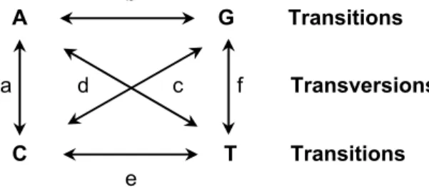
b A G Transitions a d c f Transversions C T Transitions e
Figure 3 – Substitution matrix representing the possible different rates of evolution for
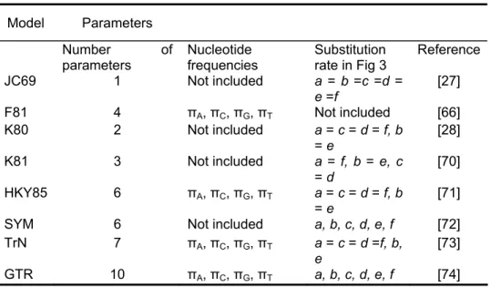
Table 3 shows some of the most commonly used nucleotide substitution models. Model parameters can reflect differences in nucleotide frequencies, substitution rate and among-site rate variation. The different rates of evolution
between specific nucleotide pairs9 are represented by the substitution matrix of
the model, and the gamma distribution models among-site rate variation [68,69] (that is the overall substitution rate at a nucleotide site). The statistical representation of rate variation is independent of substitution models and can simply be added to a pre-existing model [25].
Table 3 – Some commonly used models of nucleotide substitution. In Bos et al [25].
Model Parameters Number of
parameters Nucleotide frequencies Substitution rate in Fig 3 Reference
JC69 1 Not included a = b =c =d = e =f [27] F81 4 πA, πC, πG, πT Not included [66] K80 2 Not included a = c = d = f, b = e [28] K81 3 Not included a = f, b = e, c = d [70] HKY85 6 πA, πC, πG, πT a = c = d = f, b = e [71]
SYM 6 Not included a, b, c, d, e, f [72]
TrN 7 πA, πC, πG, πT a = c = d =f, b,
e
[73]
GTR 10 πA, πC, πG, πT a, b, c, d, e, f [74]
The fit of the evolution model to the data may affect the performance of the model-based phylogenetic method [67]. Specially when dealing with divergent sequences, the use of one model over another can alter the result of the analysis, ultimately producing strong support for the wrong tree topology [75]. The use of objective criteria to select the model helps avoiding problems associated with model over-fitting and phylogenetic bias by selecting more realistic models [76]. Methods for selecting the best fit model for a particular data set have been proposed. Two of the most used are the likelihood ratio test (LRT) [67,76] and the Akaike information criterion (AIC) [77].
9 Like for example the special case of bacteriophage T7 propagation in the conditions described in
chapter 3, which are known to bias nucleotide substitution favouring two special cases of transitions: from G → A and C → T.
The LRT statistic is calculated by obtaining the likelihood scores of a null
model (L0) and an alternative model (L1). The two scores are then compared
by calculating the statistic δ:
(
ln
1ln
0)
2
L
−
L
=
δ
(16)
When the compared models are nested, the Chi-square distribution is a good approximation of the null distribution of the LRT statistic (df = difference in the number of free parameters in the two models). LRT requires an a priori input phylogeny to estimate the likelihood of the models [78].
The Akaike information criterion is another way of selecting the most appropriate model for a data set. It represents the amount of information lost when a particular model is used to approximate reality. The AIC implements best-fit model selection by calculating the likelihood of proposed models and imposing a penalty based on the number of model parameters. Parameter-rich models are penalized so fitting an excessively complex model is not likely under this criterion. The best fitting model is the one with the smallest AIC value.
(
L
iN
i)
AIC
=
−
2
ln
+
2
(17)
Where Li is the likelihood for model i and Ni is the number of free parameters
in model i. The AIC has the advantage over LRT of simultaneously comparing all candidate models and also has an adjustment that more heavily penalizes complex models for data comprised of small samples (short sequences) [25].
1.3.3.2 Assessing confidence – bootstrap
The most widely used method of estimating the reliability of trees is the nonparametric bootstrap [79]. The reliability of the tree topology (how strongly does the data support the relationships depicted in the tree) is addressed by this method through the calculation of the bootstrap percentage (BP) for each interior node, or clade, in a tree. The data set (sites in a set of aligned sequences) is randomly sampled with replacement to create pseudo-replicate data sets. The tree building algorithm is performed on each of these replicate data sets. Typically, 100-2000 bootstrap trees are estimated, and the BP for each clade (on the original phylogenetic tree) is the percentage of these trees that also include that clade. The bootstrap offers a measure of which clades are weakly supported, since a grouping that is present in a low percentage of
![Figure 2 – Tree with branch lengths and data at a single site. In Felsenstein (2004) [1]](https://thumb-eu.123doks.com/thumbv2/123dok_br/19239637.970925/36.723.158.597.551.955/figure-tree-branch-lengths-data-single-site-felsenstein.webp)