UNIVERSIDADE DA BEIRA INTERIOR
Ciências Sociais e Humanas
The nexus between financial development and
economic growth: A panel-VAR evidence
Nuno Miguel Dias Filipe
Dissertação para obtenção do Grau de Mestre em
Economia
(2º Ciclo de Estudos)
Orientador: Prof. Doutor José Alberto Serra Ferreira Rodrigues Fuinhas
iii
Dedication
In memory of Mia Maria José do Couto Guterres
v
Acknowledgments
First and foremost, I wish to thank my supervisor Professor Doutor José Alberto Fuinhas, whom without is immeasurable support, comprehension, guidance, and incentive this dissertation would not have been possible. He has taught me economic theories, concepts and econometric skills to improve and increase my knowledge, I have been fortunate with is friendship and with the possibility to learn with him.
Second my words go out to my family for all their love, encouragement and incentive. To my parents who raised me and gave me all the love and guidance for life. Special to my mom who always believed in me and gave me all the strength and support to fight all the adversities and to follow my dreams. To Edite for all her love, support and encouraging, for believing in me and gave moral and emotional support along this journey.
Last but not least, I would like to express my gratitude to my good friends, who I had the privilege do meet along this journey and were always there in good and in the bad moments. A special thanks to Cátia Lopes, André Branco and Matheus Belucio for all the support and incentive, and for being my friends.
vii
Resumo
Este estudo examina a relação entre crescimento económico, inflação, abertura económica e financeira, desenvolvimento do sector bancário e do mercado de ações, através da elaboração de um painel de seis países (Espanha, França, Grécia, Irlanda, Itália e Portugal), para o período de 1990-2015, com a utilização de dados anuais. Os dados foram obtidos através da base de dados dos indicadores de desenvolvimento mundial (WDI) e de desenvolvimento financeiro global (GFDD), publicados pelo World Bank e pelo fundo monetário internacional (FMI). Através do procedimento de análise de componentes principais (PCA), elaborou-se duas novas variáveis para medir o desenvolvimento do setor bancário e o desenvolvimento do mercado acionista (compostos por diversas variáveis). As restantes variáveis em estudo são o PIB per capita, a inflação, o comércio e o investimento direto estrangeiro proposto como medida de facto, utilizando um modelo em painel PVAR, para testar a causalidade à Granger e interdependência entre as variáveis, assim como a presença entre as variáveis de causalidade unidirecional e/ou bidirecional. Este estudo tem como foco uma melhor compreensão na relação entre as variáveis em estudo assim como um grupo de países afetados pela crise do subprime, ainda não estudados em conjunto. Conclui-se que o desenvolvimento do setor bancário do mercado acionista e o grau de abertura económico contribui positivamente para o crescimento económico, não se detetando causalidade do grau de abertura financeiro para o crescimento.
Palavras-chave
Desenvolvimento Financeiro; Crescimento Económico; Abertura Financeira; Abertura Económica; Painel-VAR
ix
Resumo alargado
Os fatores que estimulam e influenciam o crescimento económico, são de particular interesse para os investigadores. O desenvolvimento financeiro é, desde os pioneiros estudos realizados por Schumpeter (1911), identificado como impulsionador positivo de crescimento económico, posteriormente estudos realizados por McKinnon (1973) e Shaw (1973) reforçaram o aspeto positivo desse output. Predominantemente estudos realizados em contexto macroeconómico são para determinar fatores de crescimento económico (Bassanini, Scarpetta and Hemming, 2001; Goldsmith, 1969; Levine, 1991; Pagano, 1993).
Com as constantes alterações evolutivas existentes, sejam elas provocadas pelos avanços tecnológicos, pelo desenvolvimento dos países, surgimento de novos mercados, etc…, os fatores que potenciam o crescimento económico, são diversificados. Assim Barro e Sala-i-Martin (1995), Romer (1998) or Yucel (2009) realizaram estudos sobre abertura e crescimento económicos. Foram ainda construídos índices compostos por um leque de variáveis para analisar o impacto do desenvolvimento do setor bancário e do mercado acionista no crescimento económico (Fink, Haiss, & Vuksic, 2009; Beck & Levine, 2004; Levine & Zervos, 1998; Yartey, 2008). Importa ainda destacar estudos empíricos que relacionam a inflação com o crescimento económico (Barro, 2013, Boujelbene & Boujelbene, 2010 e Jalil, Tariq, & Bibi, 2014).
Contudo, os investigadores deparam-se com a dificuldade em identificar as relações de causalidade entre as variáveis (o crescimento económico é potenciado pelas variáveis ou vice-versa). É possível identificar, na literatura em termos de direção, quatro tipos de hipóteses: hipótese neutra (sem relação de causalidade), supply-leading e demand-following (existência de causalidade unidirecional) e a hipótese feedback (causalidade bidirecional), (Pradhan et al., 2013, 2014 e 2017).
Com base nas premissas anteriores, este estudo investiga a causalidade entre o crescimento económico, a inflação, a abertura económica e financeira e de duas componentes financeiras: desenvolvimento do setor bancário e desenvolvimento do mercado de ações. Elaborou-se um painel de seis países europeus (Espanha, França, Grécia, Irlanda, Itália e Portugal) selecionados pelas suas semelhanças culturais e históricas, assim como pelo fato de serem economias afetadas pela crise do subprime, com recolha de dados anuais para o período de 1990-2015. Os dados utilizados foram recolhidos da base de dados dos indicadores de desenvolvimento mundial (WDI) e de desenvolvimento financeiro global (GFDD), publicados pelo World Bank e pelo fundo monetário internacional (FMI). As variáveis usadas em estudo foram transformadas em valores per capita, seguido dos logaritmos naturais e em primeiras diferenças, e são: o PIB per capita, a inflação, o comércio e o investimento direto estrangeiro proposto como medida
x de facto. Foi ainda possível elaborar duas novas variáveis para medir o desenvolvimento do setor bancário e o desenvolvimento do mercado acionista, com incorporação de cinco componentes no BSD e de quatro no SMD (uma das componentes foi rejeita pelo PCA). Esse procedimento foi efetuado com recurso à análise de componentes principais (PCA), utilizando-se o teste de Bartlette e o teste de adequabilidade de Kaiutilizando-ser-Meyer-Olkin, como avaliação da adequabilidade do PCA. Salientar a inclusão de duas shift dummy com o valor 1 para capturar os efeitos da adesão dos países à União Monetária, e os efeitos da crise do subprime. Foram ainda realizados outros testes preliminares como: o teste Pesaran, que testa a dependência seccional - cross section dependence, o teste VIF para testar a multicolinearidade e ainda o teste de Hausman, para testar a opção entre efeitos fixos ou aleatórios.
Para testar a causalidade à Granger, a interdependência entre as variáveis e a presença de causalidade unidirecional e/ou bidirecional entre as variáveis, utilizou-se um modelo em painel desenvolvido por Love & Zicchino (2006) - PVAR (painel vetor autorregressivo). Este modelo tem implícito como estimador o Método Generalizado dos Momentos (GMM). Destacar que a validação dos dados foi efetuada pela função impulso-resposta, pela condição de estabilidade
eigenvalue e pela previsão-erro decomposição da variância.
Após execução dos testes de diagnostico, estimou-se o modelo e procedeu-se à validação dos resultados, concluindo-se que o crescimento económico contribui positivamente para o desenvolvimento do setor bancário do mercado acionista e para o grau de abertura económico (hipótese feedback), não se detetando causalidade (hipótese neutra) do crescimento económico para o grau de abertura financeiro. O resultado de hipótese neutra obtido, deve-se em muito pelo fato de o indicador sere fortemente influenciado pelos mercados e investidores estrangeiros, uma vez que o investimento direto estrangeiro foi utilizado como proxy para medir a abertura financeira.
Da análise efetuada ao teste função impulso-resposta destacar que as variáveis apresentam na generalidade uma resposta positiva aos choques, e que após a ocorrência do mesmo, a maioria das recupera num período de 4 anos (salvo alguma exceção). Da previsão-erro decomposição da variância é ainda possível destacar que as variáveis são autoexplicadas, e que o PIB per capita, a inflação e o desenvolvimento do mercado acionista recuperam mais de 60% após o choque num período de 8 anos. Exceção feita ao desenvolvimento do sector bancário e do mercado acionista, o PIB per capita é a variável que melhor responde aos choques.
xii
Abstract
This study examines the relationship between economic growth, inflation, economic and financial openness, banking sector development and stock market development through a panel of six countries (France, Greece, Ireland, Italy, Portugal and Spain) for the period 1990-2015, using annual data. The data was gathered from the GFDD (Global Financial Development Database), WDI (World Development Indicators) both published by the World Bank and from IMF (International Monetary Fund). By using principal component analysis (PCA) was possible to construct two new measures, one for banking sector development, and other for stock market development, with several component’s each, the rest of the variables are the GDP per capita, inflation, trade, foreign direct investment proposed as a de facto measure. A panel vector auto-regressive (PVAR) model was used to test Granger causalities and the interdependence between variables as well as the presence of unidirectional and bidirectional causality between the variables. This study contributes for a better understanding between the relationship of the variables used and with a role of countries affected with the subprime crises, not yet studied together. Results show that the economic growth have a positive contribute to banking sector development, stock market development and to economic openness, however there was no causality from economic growth to financial openness.
Keywords
xiv
Table of contents
1. Introduction ... 1
2. Literature Review ... 3
3. Data and methodology ... 7
3.1. Data ... 7
3.2. Methodology ... 11
4. Empirical results ... 14
5. Conclusion ... 19
xvi
Figures List
Figure 1: Relationship between all variables. ... 10
Figure 2: Econometric test and methodology realized. ... 12
Figure 3: Causality resume between the variables – according statistical significance. ... 15
Figure 4: Impulse response functions. ... 16
xviii
Tables List
Table 1: Resume of the studies on causality between several variables and economic growth. 4
Table 2: Variables description. ... 9
Table 3: Description of variables used in composite index of banking sector development. .... 9
Table 4: Description of variables used in composite index of stock market development. .... 10
Table 5: Test of sphericity and sampling adequacy for construction of BSD. ... 10
Table 6: Test of sphericity and sampling adequacy for construction of SMD. ... 11
Table 7: Descriptive statistics and cross-sectional dependence. ... 12
Table 8: VIF test. ... 13
Table 9: Lag order selection. ... 13
Table 10: Hausman test. ... 13
Table 11: Results estimation... 14
xx
Acronyms List
BSD - banking sector development CPI – consumer price index FDI – foreign direct investment GDP - gross domestic product
GFDD – global financial development database GMM - generalized method of moments IMF - international monetary fund INF – inflation
MU – monetary union
OECD - organisation for economic co-operation and development PCA - principal component analysis
PVAR - panel vector auto-regressive SMD - stock market development VIF - variance inflation test WDI – world development indicators
1
1. Introduction
Economic growth, during the last decade’s academic researchers, gave a great deal of attention to this subject, analysing and connect it with several economic outputs to better comprehend and perceive it. Along with economic growth, financial development has also been a very important subject for researchers, since the begging of the 20th century, when Schumpeter (1911) presented his work in which he shows the positive linkage between them, later also McKinnon (1973) and Shaw (1973) when studied the welfares of financial repression related economic growth and finance, almost every study in macroeconomic context, relate empirical determinants of economic growth (e.g. Bassanini, Scarpetta and Hemming, 2001; Goldsmith, 1969; Levine, 1991; Pagano, 1993).
Never the less, with the constant changes in the world regarding the improvements in technology, better communications (e.g. WWW1), advances in transport, emergence of new markets (e.g. EU2), that leads to global markets the economic growth subject is now wider than ever, so studies like Barro and Sala-i-Martin (1995), Romer (1998) or Yucel (2009) over trade openness is now very important. As important measure, there is also SMD (Stock Market Development), and BSD (Banking Sector Development), each one with their components, identify by the empirical literature as related with economic growth (Fink, Haiss, & Vuksic, 2009; Beck & Levine, 2004; Levine & Zervos, 1998; Yartey, 2008).
Economic researchers like Barro (2013), Boujelbene & Boujelbene (2010) or even Jalil, Tariq, & Bibi (2014), agree that inflation has consequences for economic growth (e.g. studies demonstrate that a controlled and stable inflation facilitates investments and business decisions).
It is also worth mentioning more recent studies that link economic growth with financial openness, by using financial indicators à de facto developed by Lane and Milesi-Ferretti (2007) like the study from Herwartz and Walle (2014), Zhang, Zhu & Lu (2015) or à de jure proposed by Chinn and Ito (2006), like the study of Andreasen and Valenzuela (2016), Rodriguez (2017). The contribution of these study has two major aspects, the first is that analyses a panel of six European countries who suffered from the subprime mortgage crisis started in the USA3, and the time span allows to assay the impact of becoming a member of the euro area. The second
1 WWW – World Wide Web.
2 EU - European Union – political and economic union of 28 country members located in European
continent.
2 aspect is that the study seeks to find the relation between economic growth, economic and financial openness, baking sector development and stock market development.
The number of variables used by the researchers to analyse this matters is so wide, like trade openness, government expenditure, inflation, foreign direct investment, gross capital formation imports of goods and services, infrastructures (see, for instance, Fischer 1993; Mankiw, Romer & Weil, 1992), so to realize this study was used GDP to capture the economic growth, and other important variables, such as inflation, trade openness to measure economic openness, foreign direct investment to measure financial openness, and used principal component analysis (PCA) to create two single variables to assess stock market development and banking sector development. These variables are studied over a period of twenty-six years (1990-2015) and to a panel of six country’s (France, Greece, Ireland, Italy, Portugal and Spain) by using a panel vector auto-regressive (VAR) model to capture the impulse-response functions and variance decomposition to see the shocks variables suffer in a certain time interval. The structure of this study is divided as follows. Section 2 is dedicated to the literature review, in Section 3 shows the data, methodology, construction of the composite measures BSD and SMD and the diagnostics tests, Section 4 shows the empirical results and finally on Section 5, the concluding remarks.
3
2. Literature Review
Since it’s such a wide and interest subject to study, many researchers focus their attention in economic growth and his connexion with all the others economic variables, such as baking sector development, stock market development, inflation, trade, foreign direct investment. Several studies, with different time spans and different countries where realize, which generate a sizable body of literature, so the results of the casual effect direction are vast. To better show these mixed findings throughout the literature, it’s presented a resume over the tables below.
The analyse of the interaction between economic growth and other variables has been the focus since the seminal work of Schumpeter (1911), followed by Goldsmith (1969), McKinnon (1973) and Shaw (1973), who focus in the link between economic growth and financial sector development and generate an intensive debate. After, the works of Lucas (1988) shows that financial sector only respond to economic growth. But recent literature, see Levine (1997) or Bertocco (2008) highlights the positive causality between a healthy financial system and economic growth.
However other studies like Liu and Hsu (2006), Li (2007), Cole, Moshirian and wu (2008), Rousseau and Yilmazkuday (2009) or Montes and Tiberto (2012), stress that in the long-run, stock market development is key in fostering economic growth. Inflation is also a variable often use to investigate causality between economic growth, Boujelbene & Boujelbene (2010), Barro (2013) and Jalil, Tariq, & Bibi (2014) defend that controlled and stable inflation promotes business and investment decisions. So, it’s obvious that inflation and stock market development are related.
According all the vast literature is difficult to identify if it is economic growth that drives all other variables (e.g. inflation, trade openness, foreign direct investment, banking sector development, stock market development), or if is the other way around. This way it’s possible to categorise in terms of direction of causality between the variables, four types of hypotheses • Neutrality hypothesis – when there is no causality between variables, means that the
variables are independent of each other;
• Supply-leading hypothesis – when exists unidirectional causality between variables, means causality running from variables to economic growth;
• Demand-following hypothesis - when exists unidirectional causality between variables, means causality running from economic growth to one or more variables;
• Feedback hypothesis - when there is a bidirectional causality between variables, means that the causality runs in both directions.
4 According these proposition of causal relationships, between variables and economic growth, the tables below provides a synopsis of studies confirming one or several of this hypothesis. The tables are resumed by independent variable and economic growth, so was necessary to produce five tables, to identify relationship between each variable and economic growth. Some authors elaborate tables with resume studies regarding the economic growth nexus, e.g. Pradhan, et al (2017), inspired in those authors table 1 below highlighted the aspects of the literature in which studies confirmed causality between the variables (inflation, trade, foreign direct investment, banking sector development, stock market development) and economic growth. It is also indicated in the table 1 the four types of causality direction that the authors determine for each relation between the variables.
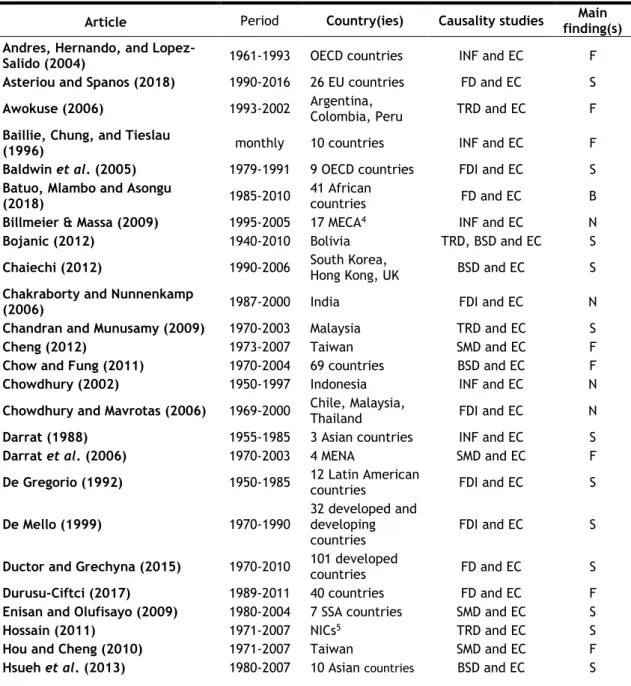
Table 1: Resume of the studies on causality between several variables and economic growth.
4 MECA - Middle East and Central Asia. 5 NICs - Newly-industrialized countries.
Article Period Country(ies) Causality studies finding(s) Main
Andres, Hernando, and
Lopez-Salido (2004) 1961-1993 OECD countries INF and EC F
Asteriou and Spanos (2018) 1990-2016 26 EU countries FD and EC S
Awokuse (2006) 1993-2002 Argentina, Colombia, Peru TRD and EC F
Baillie, Chung, and Tieslau
(1996) monthly 10 countries INF and EC F
Baldwin et al. (2005) 1979-1991 9 OECD countries FDI and EC S
Batuo, Mlambo and Asongu
(2018) 1985-2010
41 African
countries FD and EC B
Billmeier & Massa (2009) 1995-2005 17 MECA4 INF and EC N
Bojanic (2012) 1940-2010 Bolivia TRD, BSD and EC S
Chaiechi (2012) 1990-2006 South Korea, Hong Kong, UK BSD and EC S
Chakraborty and Nunnenkamp
(2006) 1987-2000 India FDI and EC N
Chandran and Munusamy (2009) 1970-2003 Malaysia TRD and EC S
Cheng (2012) 1973-2007 Taiwan SMD and EC F
Chow and Fung (2011) 1970-2004 69 countries BSD and EC F
Chowdhury (2002) 1950-1997 Indonesia INF and EC N
Chowdhury and Mavrotas (2006) 1969-2000 Chile, Malaysia, Thailand FDI and EC N
Darrat (1988) 1955-1985 3 Asian countries INF and EC S
Darrat et al. (2006) 1970-2003 4 MENA SMD and EC F
De Gregorio (1992) 1950-1985 12 Latin American countries FDI and EC S
De Mello (1999) 1970-1990
32 developed and developing countries
FDI and EC S
Ductor and Grechyna (2015) 1970-2010 101 developed countries FD and EC S
Durusu-Ciftci (2017) 1989-2011 40 countries FD and EC F
Enisan and Olufisayo (2009) 1980-2004 7 SSA countries SMD and EC S
Hossain (2011) 1971-2007 NICs5 TRD and EC S
Hou and Cheng (2010) 1971-2007 Taiwan SMD and EC F
5
6 SSA - sub-Saharan African
7 ASEAN - Association of Southeast Asian Nations. 8 MENA - Middle East and North Africa region.
9 OECD - Organisation for Economic Co-operation and Development. 10 BRICS - Brazil, Russia, India, China and South Africa.
11 MMs – Mature Markets. 12 EMs - Emerging Markets.
Ibrahim and Alagidede (2018) 1980-2014 29 SSAcountries6 FD and EC F
Jayanthakumaran and Verma
(2008) 1967-2005 ASEAN7 5 TRD and EC D
Kar et al. (2011) 1980-2007 15 MENA countries BSD, SMD and EC D
Kar, Nazlioglu, and Agir (2011) 1980-2007 MENA8 countries INF and EC F
Khaliq and Noy (2007) 1998-2006 Indonesia FDI and EC D
Kim, Lim and Park (2013) 1985-2002 Korea INF and EC D
Kolapo and Adaramola (2012) 1990-2010 Nigeria SMD and EC S
Konya (2006) 1960-1997 24 OECD countries TRD and EC F and D
Liu and Sinclair (2008) 1972-2003 China SMD and EC D
Manuchehr and Ericsson (2001) 1970-1997 4 countries FDI and EC N
Menyah et al. (2014) 1965-2008 21 African countries BSD and EC S
Nguyen and Wang (2010) 1991-2006 Taiwan INF and EC D and F
Odhiambo (2008) 1969-2005 Kenya SMD and EC D
Odhiambo (2010) 1969-2006 South Africa BSD and EC D
Ono (2017) 1999-2014 Russia FD and EC D
Ouyang and Li (2018) 1996-2015 30 Chinese provinces FD and EC S
Panopoulou (2009) 1995-2007 5 countries BSD, SMD and EC D
Pradhan et al. (2018) 1989-2015 23 EU countries FD and EC S
Pradhan, Arvin and Bahmani
(2018) 1961-2014 49 EU countries FD and EC F
Pradhan, Arvin et al. (2013) 1988-2012 16 Asian countries SMD and EC S
Pradhan, Arvin et al. (2014) 1960-2011 Asian countries BSD and EC F
Pradhan, Arvin, and Bahmani
(2015) 1960-2012 34 OECD
9
countries INF and EC S
Pradhan, Dasguta et al.(2013) 1989-2011 5 BRICScountries 10 BSD and EC F
Pradhan, Mukhopadhyay et al.
(2013) 1961-2011
15 Asian
countries BSD and EC D
Rashid (2008) 1994-2005 Pakistan SMD and EC F
Ruiz (2018) 1991-2014 116 countries FD and EC S
Sarkar (2007) 1970-2002 51 less developed countries FDI and EC N
Shahbaz (2012) 1971-2011 Pakistan TRD and EC S and D
Shaikh (2010) 1981-1999 47 developing countries FDI and EC D
Tang and Chea (2013) 1972-2008 Cambodia TRD and EC F
Tsouma (2009) 1991-2006 22 MMsEMs12 11 and SMD and EC S
Vaona (2012) 1960-1999 167 countries INF and EC N
Wolde-Rufael (2009) 1966-2005 Kenya BSD and EC F
Zhang (2001) 1984-1998 China FDI and EC S
Note(s): D: demand-following hypothesis; F: feedback hypothesis; N: neutrality hypothesis; S: supply-leading hypothesis. EC: economic Growth; INF: inflation; TRD: trade; FDI: foreign direct investment; FD: financial development; BSD: banking sector development; SMD: stock market development.
6 The table 1, shows that the relationship between economic growth and other variables, is a major concern for the researchers, since it has been widely studied along these recent years. Among the countries and group of countries studied researchers found causality relationship between economic growth and variables (indicate to each in the table) in several directions, i.e. depending the country and the variable it’s possible to see for ex. in Pakistan for a period 1971-2011 Shahbaz (2012), find a relation of demand-following and also supply-leading hypothesis between economic growth and trade, or, for ex: Nguyen and Wang (2010) in Taiwan for a period from 1991-2006 find a demand-following and a feedback hypothesis between inflation and economic growth. Highlight that in the most recent studies (2017, 2018) researchers give more attention to the relationship between financial development and economic growth, i.e. financial indicator it’s not segmented by banks or markets. The next section 3, present the data and methodology.
7
3. Data and methodology
To test the relationship between economic growth, inflation, economic and financial openness, banking sector development and stock market development, are the main aspects of this study, so to detect the causality between variables, the estimation it’s realized by using a panel vector auto-regressive (see Abrigo and Love 2015) with the intention to test the following three hypotheses:
• H1 - Banking sector development in the presence of stock market development granger causes economic growth, it’s expected to have a positive sign (i.e. BSD impulse economic growth);
• H2 - Stock market development in the presence of baking sector development granger causes economic growth, it’s expected to have a positive sign (i.e. SMD impulse economic growth); and
• H3 - Financial openness in the presence of economic openness granger causes economic growth, it’s expected to have a positive sign (i.e. FDI impulse economic growth). According the above hypotheses, this study aims to explore the economic growth nexus with, banking sector development and stock market development, for a panel of six countries (France, Greece, Ireland, Italy, Portugal, and Spain). It’s important to highlight in this study the choice of the variables where the linkage of economic growth is expanded not only to stock and banking markets, but also to economic and financial openness, and the choice of six European countries who were very affect with the subprime crises. Also significant is the use of impulse response function analysis to verify variables response to shocks. This following section 3 it’s organized in subsection 3.1 – data, variables source and description, and 3.2 – methodology applied and is explanation.
3.1. Data
First, the data was obtained from three main sources, from GFDD13 (Global Financial
Development Database) and WDI14 (World Development Indicators) both published by the World Bank and from OECD database and it covers a period from 1990-2015 (restricted to this time span because of available data).
13 GFDD - database of financial system characteristics for 214 economies, and it contains annual data,
starting from 1960.
14 WDI – database of statistical data for over 200 economies, and it contains over 1500 development
8 Second, to create the data panel, was selected six countries to analyse: France, Greece, Ireland, Italy, Portugal and Spain. The three main reasons to use these selected countries is the fact that they all are European countries with similar culture and history, they all suffered from economic and political changes along the analyses period, changes like joining the Monetary Union (MU), officially called the euro area, and finally because the six of them suffered the subprime crises (more depth crises in Greece and Portugal with the need of foreign assistance from IMF15) that caused serious damage to the financial markets and infected the real economy. Third, is important to highlight the use of dummies tool in this study, to capture the effects of two main situations: (i) integration of the six countries in the Monetary Union (MU), because for all of them was necessary to have monetary stability (relevant for integration); issues created by the physical change of the currency, etc…; (ii) economic distortion caused by the subprime crises which leads to foreign assistance in some cases (Portugal and Greece). The dummies (ID16 and SD17) used to absorb structural framework impacts were applied to year 2000/2001 to capture (i) effects and adopts the number 1 value, for the (ii) effects applied a dummy with a number 1 value for the year 2008 – 2010.
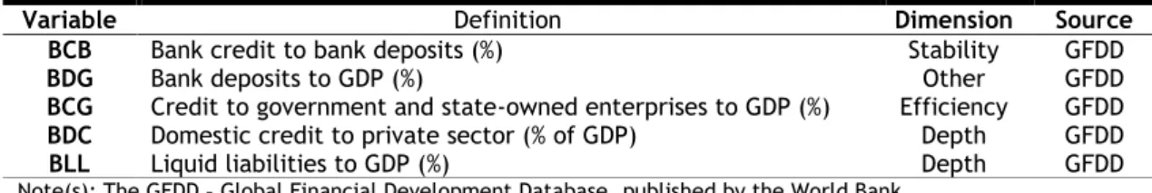
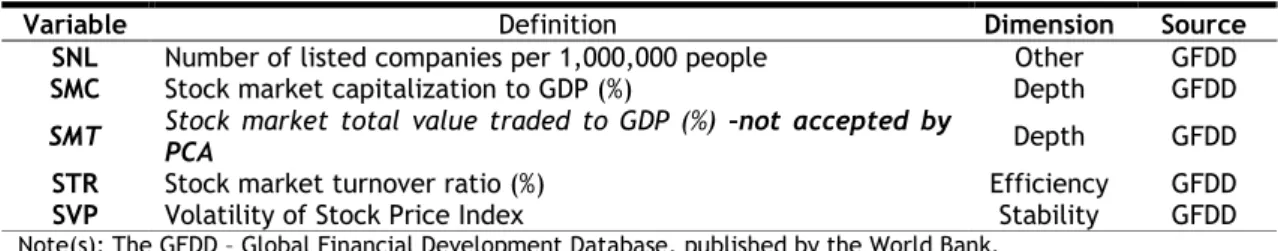
Fourth, the principal variable of this study is the real gross domestic product per capita at constant LCU18 used as a proxy to measure economic growth, followed by the other variables selected such as inflation measured by consumer price index (CPI19) as a proxy to measure inflation. The trade (i.e., exports plus imports) % of GDP used to proxy economic openness. As a proxy to financial openness its used the sum of foreign assets and liabilities over GDP constructed with the foreign direct investment, net inflows (% of GDP) plus the foreign direct investment, net outflows (% of GDP), proposed as de facto measure by Lane and Milesi-Ferretti (2007), that has been adopted instead of a de jure measure because of the available data and because is less vulnerable to endogeneity. Finally, to distinguish between the two components of financial sector (BSD, SMD), it’s created an index derived from other measures (commonly used measures over the literature) using the principal component analysis. Since the financial sector is multifaceted, any credible measure of financial development must incorporate four financial dimensions, such as depth, efficiency, stability and others to get a better accuracy of measurement.
So considering all the aspects above, the composite measure for the banking sector development (BSD) is created with: (i) bank credit to bank deposits (%) – stability dimension; (ii) bank deposits to GDP (%) – other dimension; (iii) credit to government and state-owned enterprises to GDP (%) – efficiency dimension; (iv) domestic credit to private sector (% of GDP) – depth dimension; (v) liquid liabilities to GDP (%) – depth dimension; and the stock market development (SMD) is created with: (i) number of listed companies per 1,000,000 people - other
15 IMF - International Monetary Fund. 16 ID – impulse dummy
17 SD – shift dummy 18 LCU – local currency. 19 CPI – consumer price index.
9 dimension; (ii) stock market capitalization to GDP (%) - depth dimension; (iii) stock market total value traded to GDP (%) - depth dimension, a part of begin referred over the literature, this variable was not used in this composite because it was not accept by the PCA, (iv) stock market turnover ratio (%) - efficiency dimension; (v) volatility of stock price index - stability dimension. The variables were transformed in per capita values except inflation rate, foreign direct investment (constructed variable), number of listed companies per 1,000,000 people, and volatility of stock price index. After they were transformed in their natural logarithm form, following by their first differences for estimation, except inflation rate, number of listed companies per 1,000,000 people and volatility of stock price index.
Table 2 shows the variables definition and source, three of the variables were selected from World Development Indicators and another three from the Global Financial Development Database, both published by the World bank, only one of the variables was gather from Organisation for Economic Co-operation and Development.
Table 2: Variables description.
Variable Definition Source
GDP GDP per capita (constant LCU) WDI
INF Inflation measured by consumer price index (CPI) OECD
FDI Foreign direct investment, net inflows + net outflows (% of GDP) WDI
TRD Trade (% of GDP) WDI
BSD Composite index of banking sector development (using five variables) GFDD
SMD Composite index of stock market development (using five variables) GFDD
Note(s): WDI - World Development Indicators, published by the World Bank, GFDD - Global Financial Development Database, published by the World Bank, OECD - Organisation for Economic Co-operation and Development.
Through the mathematical procedure of principal component analysis that transforms a previous group of correlated variables into a small group who keeps most of the possible variance from the first group (i.e. this technique creates a single variable, with the essential information removed from each variable). So, to create a composite index through PCA for BSD and SMD, it’s used the variables indicated in table 3 and 4.
In table 3, it is highlighted the variables used to create the composite index of banking sector development, source definition (all of them gathered from the Global Financial Development Database, published by the World Bank) and correspondent financial dimensions.
Table 3: Description of variables used in composite index of banking sector development.
Variable Definition Dimension Source
BCB Bank credit to bank deposits (%) Stability GFDD
BDG Bank deposits to GDP (%) Other GFDD
BCG Credit to government and state-owned enterprises to GDP (%) Efficiency GFDD
BDC Domestic credit to private sector (% of GDP) Depth GFDD
BLL Liquid liabilities to GDP (%) Depth GFDD
10 In table 4, it is highlighted the variables used to create the composite index of stock market development, source definition (all of them gathered from the Global Financial Development Database, published by the World Bank) and correspondent financial dimensions.
Table 4: Description of variables used in composite index of stock market development.
Variable Definition Dimension Source
SNL Number of listed companies per 1,000,000 people Other GFDD
SMC Stock market capitalization to GDP (%) Depth GFDD SMT Stock market total value traded to GDP (%) –not accepted by PCA Depth GFDD
STR Stock market turnover ratio (%) Efficiency GFDD
SVP Volatility of Stock Price Index Stability GFDD
Note(s): The GFDD – Global Financial Development Database, published by the World Bank.
The figure 1 shows the relationship between variables, correspondent definitions, the circles correspond to the primary variables under study, the squares figures indicates the variables that compose the PCA.
Figure 1: Relationship between all variables20.
The robustness of the composite index Banking Sector Development (BSD) was verified by the application of Bartlett’s test for sphericity (Bartlett, 1950) and Kaiser-Meyer-Olkin of sampling adequacy (Kaiser, 1970), table 5 present the results of the test.
Table 5: Test of sphericity and sampling adequacy for construction of BSD.
Construction of BSD
Bartlett test of sphericity
Chi-square 1199.706
Degree of freedom 10
p-value 0.000
Determinant of the correlation matrix 0.000
Kaiser-Meyer-Olkin measure of sampling adequacy
0.624
11 For the BSD index the Kaiser-Meyer-Olkin21 measure of sampling adequacy indicates a value of 0.642, so it’s possible to apply the PCA. In the case of the Bartlett’s22 test for sphericity the null hypothesis was rejected with a p-value less than 5% (0.000) and a Chi-square distributed it’s statistical significant and it shows that the variables are significant correlated.
The robustness of the composite index Stock Market Development (SMD) was verified by the application of Bartlett’s test for sphericity (Bartlett, 1950) and Kaiser-Meyer-Olkin of sampling adequacy (Kaiser, 1970), table 6 present the results of the test.
Table 6: Test of sphericity and sampling adequacy for construction of SMD.
Construction of SMD
Bartlett test of sphericity
Chi-square 58.202
Degree of freedom 6
p-value 0.000
Determinant of the correlation matrix 0.667
Kaiser-Meyer-Olkin measure of sampling adequacy
0.569
For the SMD index the Kaiser-Meyer-Olkin measure of sampling adequacy indicates a value of 0.569, so it’s possible to apply the PCA. In the case of the Bartlett’s test for sphericity the null hypothesis was rejected have a p-value less than 5% (0.000) and a Chi-square distributed it’s statistical significant and it shows that the variables are significant correlated.
3.2. Methodology
In this study is applied a technique that combines the regular VAR approach, that treats as endogenous all the variables in the system, with the unobserved individual heterogeneity from a panel-data approach (Grossmann et al., 2014). The application of a panel data vector autoregressive (PVAR) model was developed by Love & Zicchino (2006), and it’s used the same methodology. The mentioned model, a first-order PVAR, uses an equation stated as follows in eq. 1:
𝑧𝑖𝑡 = Γ0+ Γ1𝑧𝑖𝑡−1+ 𝑓𝑖+ 𝑑𝑐,𝑡+ 𝑒𝑡 (1)
Where, 𝑧𝑡 is vector variables, in this study they are: dlGDP, INF, dlTRd, dlFDI dlBSD and dlSMD. All variables are in natural logarithm following by their first differences except INF (inflation), dlGDP denotes gross domestic product per capita, proxy for economic growth; INF represents inflation measured by consumer price index, proxy for inflation; dlTRD the ratio of trade to GDP as a proxy for economic openness; dlFDI foreign direct investment (% GDP) as proxy for financial openness; dlBSB and dlSMD is a created index for banking sector development and stock market development respectively. Γ0 correspond to the constant vector, Γ1𝑧𝑖𝑡−1 to the
21 Result value between 0 and 1 and if the output is below 0.5 the PCA must not be applied. 22 The null hypothesis is that variables are not intercorrelated.
12 matrix polynomial, 𝑓𝑖 the fixed effects in the model, 𝑑𝑐,𝑡 the effects of time, and the term of random errors is 𝑒𝑡.
A technique applied by Love & Zicchino (2006) called "Helmert Procedure" (Arellano & Bover, 1995), to solve the problem of fixed effects correlated with the regression related to delays of the dependent variables, usually average differentiation procedure is used to eliminate fixed effects, is also used in the model to avoid occur biased coefficients.
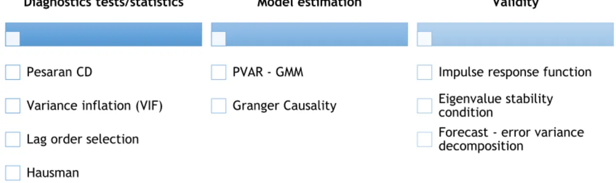
Once it’s very important econometric analysis and it requires several tests before and during the estimating the model, figure 2, describes the methodology used in this study.
Figure 2: Econometric test and methodology realized.
To improve the construction and estimation of the PVAR model it’s necessary to conduct preliminary analysis. Starting with the test for panel cross-sectional dependence, through the CD23 test Pesaran (2004). Table 7, presents the descriptive statistics and cross-sectional dependence.
Table 7: Descriptive statistics and cross-sectional dependence.
Descriptive statistics Cross-sectional dependence (CSD)
Variable Obs Mean Std. Dev. Min Max CD-test Corr Abs(corr)
dlGDP 150 0.0141657 0.0337247 -0.0942879 0.2181435 12.00*** 0.699 0.699 INF 156 3.199252 3.326068 -4.478103 20.43349 11.49*** 0.787 0.787 dlFDI 144 0.0427203 0.6799524 -2.442108 2.889361 1.83** 0.101 0.202 dlTRD 150 0.0327228 0.0773082 -0.2638502 0.2559261 11.76*** 0.680 0.680 dlBSD 147 0.1302538 0.2522549 -0.3591483 1.191323 11.51*** 0.678 0.678 dlSMD 141 0.0768329 0.4020746 -1.468099 1.238657 8.07*** 0.474 0.474
Note(s): ***, **, * denote statistical significance level of 1%, 5% and 10%, respectively. CD test has N (0,1) distribution, under the H0: cross-sectional independence.
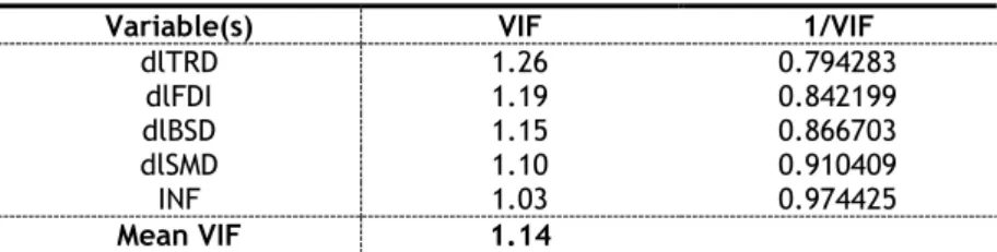
Through table seven, it’s possible to verify that in all variables exist the presence of cross-sectional dependence (CSD), consistent with the null hypothesis CD ~ N (0,1). Next, to analyse if the initial requirements of the model are verified it’s performed the VIF24 test to detect the
23 CD - cross-sectional.
24 VIF - Variance Inflating Factor.
Diagnostics tests/statistics
Pesaran CD
Variance inflation (VIF) Lag order selection Hausman
Model estimation
PVAR - GMM Granger Causality
Validity
Impulse response function Eigenvalue stability condition
Forecast - error variance decomposition
13 multicollinearity. The average VIF statistic should be below 10% to continue with the analysis. Table 8, describe the results of the VIF test.
Table 8: VIF test.
Variable(s) VIF 1/VIF
dlTRD 1.26 0.794283 dlFDI 1.19 0.842199 dlBSD 1.15 0.866703 dlSMD 1.10 0.910409 INF 1.03 0.974425 Mean VIF 1.14
Analysing the table eight, shows that the collinearity is not a concern, the means VIF stays under the limit value of 10%. The following table 9, show the results for the checking lag order selection procedure that is used to determinate the overall coefficient (CD).
Table 9: Lag order selection.
lag CD J J pvalue MBIC MAIC MQIC 1 .9146926 43.71402 .1765465 -124.5078 -28.28598 -67.29304
2 .9816666 . . . . .
The table nine, have the results for lag order selection that indicates MBIC and MQIC values are lower at one lag, so a first order PVAR is selected as previous stated, see Grossmann et al. (2014) procedure.
It is important to point out the existence of a structural brake on the panel that not allows to capture the Unit Root, i.e. the test doesn’t confirm the real stationary effect of the variables, so it was not performed. Apart that, Hausman test was performed to determine whether fixed effects are present, see table 10 with the results of the test.
Table 10: Hausman test.
Chi2 Prob > Chi2
Hausman
Hausman, sigmamore
13.29 0.0208 16.55 0.0054
The results of the test validate that exits fixed effects, with the variables in their first differences, consistent with the null hypothesis – difference in coefficients are not systematic. Next in section 4, the empirical results are presented.
14
4. Empirical results
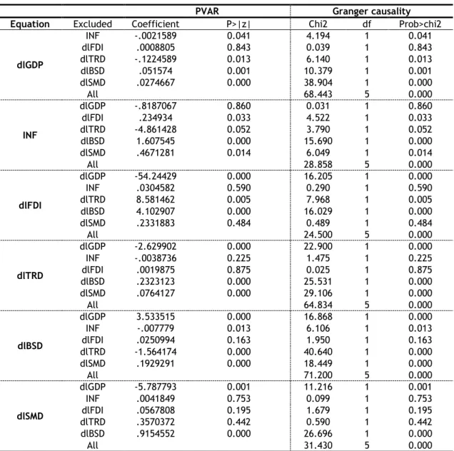
In the previous section 3, a preliminary analysis was performed to verify if the PVAR model was the most appropriate. Thus, was confirmed that the PVAR test was the most appropriate to analyse this nexus. Note that, the PVAR model was estimated using one lag and that all variables are in natural logarithms in their first differences. According Holtz-Eakin et al. (1988) the gmmst option (command) was used in the estimation (that changes missing values with zero). The PVAR Granger causality test is evaluated through a Wald test. In table 11, is possible to see the test results. The null hypothesis of the test is that excluded variable does not granger-cause equation variable.
Table 11: Results estimation.
PVAR Granger causality
Equation Excluded Coefficient P>|z| Chi2 df Prob>chi2
dlGDP INF -.0021589 0.041 4.194 1 0.041 dlFDI .0008805 0.843 0.039 1 0.843 dlTRD -.1224589 0.013 6.140 1 0.013 dlBSD .051574 0.001 10.379 1 0.001 dlSMD .0274667 0.000 38.904 1 0.000 All 68.443 5 0.000 INF dlGDP -.8187067 0.860 0.031 1 0.860 dlFDI .234934 0.033 4.522 1 0.033 dlTRD -4.861428 0.052 3.790 1 0.052 dlBSD 1.607545 0.000 15.690 1 0.000 dlSMD .4671281 0.014 6.049 1 0.014 All 28.858 5 0.000 dlFDI dlGDP -54.24429 0.000 16.205 1 0.000 INF .0304582 0.590 0.290 1 0.590 dlTRD 8.581462 0.005 7.968 1 0.005 dlBSD 4.102907 0.000 16.029 1 0.000 dlSMD .2331883 0.484 0.489 1 0.484 All 24.500 5 0.000 dlTRD dlGDP -2.629902 0.000 22.900 1 0.000 INF -.0038736 0.225 1.475 1 0.225 dlFDI .0019875 0.875 0.025 1 0.875 dlBSD .2323123 0.000 25.531 1 0.000 dlSMD .0764127 0.000 29.106 1 0.000 All 64.834 5 0.000 dlBSD dlGDP 3.533515 0.000 16.868 1 0.000 INF -.007779 0.013 6.106 1 0.013 dlFDI .0250994 0.163 1.950 1 0.163 dlTRD -1.564174 0.000 40.640 1 0.000 dlSMD .1929291 0.000 18.449 1 0.000 All 71.200 5 0.000 dlSMD dlGDP -5.787793 0.001 11.216 1 0.001 INF .0041849 0.753 0.099 1 0.753 dlFDI .0567808 0.195 1.679 1 0.195 dlTRD .3570372 0.442 0.590 1 0.442 dlBSD .9154552 0.000 26.696 1 0.000 All 31.430 5 0.000
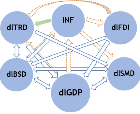
15 Figure 3, below, present a resume scheme between the variables under analyse for better clarification according the statistical significance. The blue arrow (line) indicates 1% significance, the orange arrow (dashed) 5% significance, and the green arrow (filed) 10% significance.
Figure 3: Causality resume between the variables – according statistical significance.
Therefore, according the resume on table 3, the relations between variables shows that exist a bidirectional causality (feedback hypothesis) between: (i) dlGDP and dlTRD; (ii) dlGDP and dlBSD; (iii) dlGDP and dlSMD; (iv) INF and dlBSD; (v) dlTRD and dl dlBSD; (vi) dlBSD and dlSMD, statistical significance at 1% level, except from dlGDP to dlTRD and from dlBSD to INF both statistical significance at 5% level. It also shows that exist unidirectional causality (supply-leading hypothesis) between: (i) dlGDP to INF; (ii) INF to dlFDI, dlTRD and dlSMD; (iii) dlFDI to dlGDP, dlTRD and dlBSD; (iv) dlTRD to dlSMD, statistical significance at 5% level, except from dlFDI to dlGDP, dlFDI to dlBSD and dlTRd to dlSMD statistical significance at 1% level and from INF to dfTRD statistical significance at 10% level. And finally, no causality between: (i) dlGDP to dlFDI; (ii) INF to dlGDP; (iii) dlFDI to INF, and dlSMD; (iv) dlTRD to INF and dlFDI; (v) dlBSD to dlFDI; (iv) dlSMD to INF, dlFDI and dlTRD.
So, the variable with less causality relationship is dlTRD and dlSMD, this can be explained by the fact that they are two measures that have more influence from foreign policies. In the other side the variables with more bidirectional causality connexion is dlGDP and dlBSD, this can be explained by the fact that GDP, being the proxy for economic growth should be connect with other macroeconomic variables, and BSD because have an important role over developed
16 economies, where the bank system has a huge influence over the economy (positive or negative).
In resume, is possible to mention that trade openness (dlTRD), banking sector development (dlBSD) and stock market development (dlSMD) granger-cause economic growth. Then according the previous hypotheses H1 and H2 can be proved, for H3 not valid.
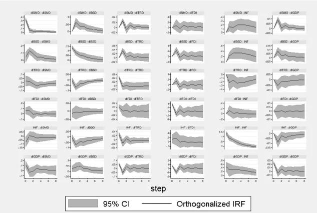
In addition, it’s possible to observe the impulse-response function. This function reveals how a variable reacts to an exogenous shock, its reactive system to measure the periods for a variable return to is equilibrium by a harmonic movement. Through the graphical analysis present in figure 4, it’s possible to verify the necessary time after a shock for a variable to return is normal form.
Figure 4: Impulse response functions.
In general, most variables after a shock recover in a 4 years’ time span. Exceptions does exist in variants but do not exceed 8 years to recover. Note that, through this graph it’s possible to verify that the variables have a positive respond to shocks, in more detail, dlGDP to trade, dlBSD and dlSMD, so it’s according to the preliminary analysis, present in the previous section. After performed a Forecast-Error Variance Decomposition (FEVD25) to show how a variable react to shocks in a specific variable (Marques, Fuinhas & Marques, 2013). The FEVD determines how much of the variance of the prediction error of each of the variables can be explained by shocks
25 FEVD - Forecast-Error Variance Decomposition – commonly used to help in the interpretation of a vector
17 exogenous with the various variables under study. Table 12, indicate with more detail this decomposition of the FEVD.
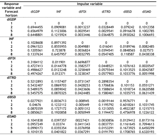
Table 12: Forecast-error variance decomposition.
Response variable and Forecast horizon Impulse variable dlGDP INF dlFDI dlTRD dlBSD dlSMD dlGDP 1 1 0 0 0 0 0 2 0.6944455 0.0909081 0.0013237 0.0328449 0.079242 0.1012358 5 0.6564979 0.1123006 0.0029541 0.0029541 0.0916678 0.1002785 8 0.6448801 0.1215924 0.0033446 0.0364875 0.0930262 0.1006693 INF 1 0.1028608 0.8971392 0 0 0 0 2 0.0961523 0.8555955 0.0049881 0.016041 0.0189746 0.0082485 5 0.1205561 0.723878 0.0036824 0.0394541 0.0848565 0.027573 8 0.1337634 0.6457957 0.0032795 0.0547405 0.118587 0.0438338 dlFDI 1 0.3184112 0.011901 0.6696877 0 0 0 2 0.4727413 0.0144778 0.3582577 0.0448521 0.1076163 0.0020547 5 0.4986627 0.0123248 0.3258469 0.0575544 0.1013525 0.0042587 8 0.4974267 0.012371 0.3238347 0.0577903 0.1033776 0.0051998 dlTRD 1 0.5212893 0.1157407 0.0731347 0.2898354 0 0 2 0.5432407 0.0869703 0.0428253 0.1706836 0.101153 0.0551271 5 0.5489375 0.0859042 0.0423606 0.1588654 0.1018734 0.0620588 8 0.5457575 0.0870325 0.0424485 0.1580461 0.1035715 0.0631439 dlBSD 1 0.0277921 0.0036713 0.008945 0.0019144 0.9576771 0 2 0.04676 0.1232112 0.005449 0.1195792 0.6018261 0.1031745 5 0.0870359 0.1727172 0.0051312 0.1213055 0.4922387 0.1215715 8 0.0850621 0.1920858 0.0050949 0.1194472 0.4756978 0.1226122 dlSMD 1 0.1041838 0.0397357 00227421 0.0030856 0.0129412 0.8173116 2 0.0957249 0.03374 0.0411343 0.0037751 0.1161645 0.7094613 5 0.0990173 0.0355354 0.0376958 0.0153291 0.1673925 0.6450299 8 0.1010135 0.0401822 0.0367291 0.0191793 0.1708765 0.6320193
The Forecast-error variance decomposition shows that in the year period the variations of the variables are explained mainly by themselves and with significant values.
Analysing the table in detail, it’s possible to find interesting situations, such as after a 2-year period, shocks to dlGDP variable explain about 69,4% of the forecast error variance, while the other variables have residuals percentages (INF – 9,1%; dlFDI – less than 1%; dlTRD – 3,3%; dlBSD – 7,9% and dlSMD – 10,1%). After an 8-year period the situation is similar, because the dlGDP stabilizes at 64,5%, and the other variables don’t change it much also (INF – 12,2%; dlFDI – still less than 1%; dlTRD - 3,6%; dlBSD - 9,3 % and dlSMD - 10%). Looking at an 8-year period shocks to INF it explains 64,6% of the forecast error variance, while the lGdDP only 13,4%, dlFDI less than 1%, dlTRD 5,5%, dlBSD 11,6% and dlSMD 4,4%. By analysing the impact on dlFDI a 10-year period shock explains 32,4%, while in the other variables have the following values, dlGDP - 49,7%; INF - 1,2%, dlTRD - 5,8%; dlBSD 10,3% and dlSMD less than 1%. Looking at dlTRD an 8-year period shock explains 15,8% of the forecast error variance, while dlGDP 54,6%, INF 8,7%, dlFDI 4,2% dlBSD 10,3% and dlSMD only 6,3%. Concerning the last two variables, first checking
18 the dlBSD with a shock at an 8-year period, explains 47,6%, while the rest is explained at dlGDP 8,5%, INF 19,2%, dlFDI less than 1%, dlTRD 11,9% and dlSMD 12,3%, second the dlSMD for an 8-year period shock explains at 63,2%, while the other variables explains at dlGDP 10,1%, INF 4%, dlFDI 3,7%, dlTRD 1,9%, dlBSD 17,1%.
In resume the most autonomous variable is dlGDP, INF and dlSMD auto explains more than 60% after 8 years period shock, dlGDP is also the variable with best response to shocks even of it happens to some other variable, except if it’s a shock regarding dlBSD or dlSMD.
A stability test was also conducted to check the estimations validation (Hamilton, 1994; Lutkephol, 2005). The results satisfy stability condition, because all eigenvalues are inside the circle unit. The eigenvalue test shows the real, imaginary and modulus values, details under figure 5. Eigenvalue Real 0.7776259 0.7776259 -0.621331 -0.4801577 0.122755 0.122755 Imaginary 0.1050486 -0.1050486 0 0 -0.2076135 0.2076135 Modulus 0.7846893 0.7846893 0.621331 0.4801577 0.2411891 0.2411891
Figure 5: Eigenvalue stability condition.
After performing the diagnostic tests, and the estimation of the PVAR model, the section 4 has validate the results obtained, so next in section 5 is possible to present a results conclusion and the contribute of this study to the economy, it’s also suggested a topic for future studies.
19
5. Conclusion
To study the dynamics and relationship between economic growth and the other variables (inflation, trade, foreign direct investment, banking sector development and stock market development) for a panel of six European countries (France, Greece, Ireland, Italy, Portugal and Spain) and a time span from 1990-2015, was applied a panel vector auto-regressive (PVAR) model to teste Granger causality, forecast-error variance decomposition and impulse-response functions.
By using a principal component analysis (PCA) mode, was possible to create two new measures, one for banking sector development (composite with a group of five variables) and other for stock market development (composite with a group of four variables), which includes four financial dimensions measures: depth, efficiency, stability and other, this way was possible to realize the study with a small set of variables and with a composite to identify specific financial markets: bank and stocks.
The variables were transformed in per capita, in their natural logarithms and in first difference for a better analyse of the causalities between them. The literature refers to four causality theories: neutrality hypothesis (no causality), supply-leading and demand-following hypotheses (unidirectional causality) and feedback hypothesis (bidirectional causality).
Remember that the following hypotheses were tested: Banking sector development in the presence of stock market development granger causes economic growth, H2 - Stock market development in the presence of baking sector development granger causes economic growth, and H3 - Financial openness in the presence of economic openness granger causes economic growth.
The estimation results respond to hypotheses according the existence of feedback hypothesis between economic growth, banking sector development, stock market development and economic openness (H1 and H2 are validate), however it also shows neutrality hypothesis between economic growth and financial openness, but a feedback hypothesis from financial openness to economic growth. So, to promote economic growth, the policies should induce a healthy and sustained external relations to help economic openness, and some good financial resources to support a good banking sector development and a healthy stock market that can captivate investors.
Seeing the impulse-response functions it’s possible to confirm that in general, after a shock, most recover in a four years’ time span (same exception in eight years). This test demonstrates that dlGDP, INF and dlSMD are the most independent variables, individual they auto explain
20 over 60% after an 8 years period shock, also the best variable reacting to shocks is dlGDP even if the shock happens to other variable, except if it’s a shock to dlBSD or dlSMD.
As a main contribute, it’s possible to refer the set of countries chosen, because they have suffered from the subprime crises, who had a huge impact over the economy and to refer the new aspect of including the economic and financial openness in the study.
For future studies is important to get a large set of countries and from different economics spheres to confirm the influence of the financial and economic openness over the economy and the contributes of the banking sector and stock market development.
21
References
Abrigo and Love (2015). Estimation of Panel Vector Autoregression in Stata: a Package of Programs. University of Hawaii working paper.
Andreasen, E., Valenzuela, P. (2016). Financial openness, domestic financial development and credit ratings. Finance Research Letters, 16, 11-18.
Andrés, J., Hernando, I., & Lopez-Salido, D. (2004). The Role of the Financial System in the Growth–inflation Link. European Journal of Political Economy, 20 (4), 941–961.
Arellano, M., & Bover, O. (1995). Another look at the instrumental variable estimation of error components models. Journal of Econometrics, 68, 29-51.
Asteriou, D., Spanos, K. (2018). The relationship between financial development and economic growth during the recent crisis: Evidence from the EU. Finance Research Letters, in press.
Awokuse, T.O. (2006). Causality between exports, imports and economic growth: evidence from transition economies. Economics Letters, 94 (3), 389–395.
Baillie, R., Chung, C., & Tieslau, M. (1996). Analyzing Inflation by the Fractionally Integrated ARFIMA-GARCH Model. Journal of Applied Econometrics, 11 (1), 23-40.
Baldwin, R., Braconier, H., Forshid, R. (2005). Multinationals, endogenous growth, and technological spillovers: theory and evidence. Review of International Economics, 13, 945–963.
Barro, R. J. (2013). Inflation and economic growth. Annals of Economics and Finance, 14 (1), 121-144.
Barro, R. J., Sala-i-Martin, X. (1995). Economic Growth. McGraw Hill. New York.
Bartlett, M. S. (1950). Tests of significance in factor analysis. British Journal of Mathematical
and Statistical Psychology, 3(2), 77-85.
Bassanini, A., Scarpetta, S., Hemming, P. (2001). Economic Growth: The Role of Policies and Institutions, Panel Data Evidence from OECD Countries. OECD Economics Department, Working Paper, p. 283.
Batuo, M., Mlambo, K., Asongu, S. (2018). Linkages between financial development, financial instability, financial liberalisation and economic growth in Africa. Research in
22 Beck, T., & Levine, R. (2004). Stock Markets, banks, and growth: Panel evidence. Journal of
Banking and Finance, 28(3), 423-442.
Bertocco, G. (2008). Finance and development: is Schumpeter's analysis still relevant? Journal
of Banking & Finance, 32 (6), 1161–1175.
Billmeier, A., & Massa, I. (2009). What Drives Stock Market Development in Emerging Markets - Institutions, Remittances, or Natural Resources? Emerging Markets Review, 10 (1), 23– 35.
Bojanic, A. N. (2012). The impact of financial development and trade on the economic growth of Bolivia. Journal of Applied Economics, 15 (1), 51–70.
Boujelbene, T., & Boujelbene, Y. (2010). Long Run determinants and short run dynamics of inflation in Tunisia. Applied Economics Letters, 17(13), 1255-1263.
Chaiechi, T. (2012). Financial development shocks and contemporaneous feedback effect on key macroeconomic indicators: A post Keynesian time series analysis. Economic
Modelling, 29(2), 487–501.
Chakraborty, C., & Nunnenkamp, P. (2006). Economic reforms, foreign direct investment and its economic effects in India. Germany: Kieler Arbeitspapiere.
Chandran, R., Munusamy (2009). Trade openness and manufacturing growth in Malaysia. Journal
of Policy Modeling, 31, 637–647.
Cheng, S. (2012). Substitution or complementary effects between banking and stock markets: Evidence from financial openness in Taiwan. Journal of International Financial Markets
Institutions and Money, 22(3), 508–520.
Chinn, M. D., Ito, H. (2006). What Matters for Financial Development? Capital Controls, Institutions, and Interactions. Journal of Development Economics, 81(1), 163-192 (October).
Chow,W.W., & Fung, M. K. (2011). Financial development and growth: A clustering and causality analysis. Journal of International Trade and Economic Development, 35(3), 1– 24.
Chowdhury, A. (2002). Does Inflation Affect Economic Growth: The Relevance of the Debate for Indonesia. Journal of the Asia Pacific Economy, 7 (1), 20-34.
Chowdhury, A., & Mavrotas, G. (2006). FDI and Growth: What Causes What? World Economy,
29(1), 9–19.
Cole, R. A., Moshirian, F., & Wu, Q. (2008). Bank stock returns and economic growth. Journal
23 Darrat, A. F. (1988). Does inflation inhibit or promote growth? Some time series evidence.
Journal of Business and Economics, 27(4), 113-134.
Darrat, A. F., Elkhal, K., & McCallum, B. (2006). Finance and macroeconomic performance: Some evidence from emerging markets. Emerging Markets Finance and Trade, 42(3), 5– 28.
De Gregorio, J. (1992). Economic growth in Latin America. Journal of Development Economics,
39, 59–84.
De Mello, L. R. (1999). Foreign direct investment-led growth: evidence from time series and panel data. Oxford Economic Papers, 51(1), 133–151.
Ductor, L., Grechyna, D. (2015). Financial development, real sector, and economic growth.
International Review of Economics & Finance, 37, 393-405.
Durusu-Ciftci, D., Ispir, M., Yetkiner, H. (2017). Financial development and economic growth: Some theory and more evidence. Journal of Policy Modeling, 39, 290-306.
Enisan, A. A., & Olufisayo, A. O. (2009). Stock market development and economic growth: Evidence from seven sub-Saharan African countries. Journal of Economics and Business,
61(2), 162–171.
Fink, G., Haiss, P., & Vuksic, G. (2009). Contribution of financial market segments at different stages of development: Transition, cohesion and mature economies compared. Journal
of Financial Stability, 5(4), 431-455.
Fischer, S. (1993). The role of macroeconomic factors in growth. Journal of Monetary
Economics, 32(3), 485-512.
Goldsmith, R. W. (1969). Financial Structure and Development. Yale University Press. New Haven, CT.
Grossmann, A., Love, I., & Orlov, A. (2014). The dynamics of exchange rate volatility: A panel VAR approach. Journal of International Financial Markets, Institutions and Money, 33, 1-27.
Hamilton, J. (1994). Time series analysis. Prentice Hall New Jersey 1994, SFB 373(Chapter 5), 837-900.
Herwartz, H., Walle, M. Y. (2014). Openness and the finance-grotwh nexus. Journal of Banking
& Finance, 48, 235-247.
Holtz-Eakin, D., Newey, W., & Rosen, H. (1988). Estimating Vector Autoregressions with Panel Data. Econometrica, 56, 1371-1395.
24 Hossain, M.S. (2011). Panel estimation for CO2emissions, energy consumption, economic growth, trade openness, and urbanization of newly industrialized countries. Energy
Policy, 39(11), 6991–6999
Hou, H., & Cheng, S. Y. (2010). The roles of stock market in the finance-growth nexus: Time series cointegration and causality evidence from Taiwan. Applied Financial Economics,
20(12), 975–981.
Hsueh, S., Hu, Y., & Tu, C. (2013). Economic growth and financial development in Asian countries: A bootstrap panel granger causality analysis. Economic Modelling, 32(3), 294– 301.
Ibrahim, M., Alagidede, P. (2018). Nonlinearities in financial development–economic growth nexus: Evidence from sub-Saharan Africa. Research in International Business and
Finance, 46, 95-104.
Jalil, A., Tariq, R., & Bibi, N. (2014). Fiscal deficit and inflation: New evidences from Tunisia.
Journal of Policy Modelling, 36(1), 883-898.
Jayanthakumaran, K., Verma, R. (2008). International Trade and Regional Income Convergence: The ASEAN-5 Evidence. Research Online (http://ro.uow.edu.au/commpapers/479). Kaiser, H. F. (1970). A second generation little jiffy. Psychometrika, 35(4), 401–415.
Kar, M., Nazlioglu, S., & Agir, H. (2011). Financial development and economic growth nexus in the MENA countries: Bootstrap panel granger causality analysis. Economic Modelling,
28 (1-2), 685-693.
Khaliq, A., & Noy, I. (2007). Foreign direct investment and economic growth: Empirical evidence from sectoral data in Indonesia. Retrieved from http://www.economics.hawaii.edu/research/workingpapers/WP_07-26.pdf.
Kim, S., Lim, H., & Park, D. (2013). Does Productivity Growth Lower Inflation in Korea? Applied
Economics, 45 (29), 2183-2190.
Kolapo, F. T., & Adaramola, A. O. (2012). The impact of the Nigerian capital market on economic growth (1990–2010). International Journal of Developing Societies, 1(1), 11– 19.
Kónya, L. (2006). Exports and growth: Granger causality analysis on OECD countries with a panel data approach. Economic Modelling, 23(6), 978–992.
Lane, P. R., Milesi-Ferretti, G. M. (2007). The external wealth of nations mark II: Revised and extended estimates of foreign assets and liabilities, 1970–2004, Journal of International
Economics, 73, 223-250 (November).