INFORMATION VALUE OF EU-WIDE STRESS TESTS
How did the market react to stress test results?
Ricardo Jorge Santos Alves
Dissertation subbmitted as partial requirement for the conferral of Master in Finance
Supervisor:
Prof. Doutor José Joaquim Dias Curto, Associate Professor, ISCTE Business School, Department of Quantitative Methods
Co-supervisor:
Prof. Doutor Paulo Viegas de Carvalho, Invited Assistant Professor, ISCTE Business School, Department of Finance
ii
IN
FORM
AT
IO
N
VALU
E
O
F
EU
-W
IDE
ST
R
ES
S TESTS
R
ic
ar
d
o J
or
ge
S
an
tos
Alv
es
iii
Abstract
In last several years the world has been facing a tremendous financial crisis which had its highlight with Lehman Brothers bankruptcy in 2008. Also Europe has been struggling with sovereign debt crisis from countries such as Ireland, Greece, Portugal, and Spain leading to weakness the whole European banking system. Therefore, regulatory entities likely European Commission or European Banking Authority had to supervise more clearly, and efficiency the whole European system banking. In order to do so and coordinated with other financial and banking entities they conducted stress tests to financial institutions between 2009 and 2011.
The aim of this dissertation is to assess if the stress tests conducted only in 2010 and 2011 had impact on financial markets. For that was constituted a portfolio of 49 banks, selected under certain criteria, and afterward portfolio returns were subjected to statistical tests using event study standard methods. Also the variation before and after tests release of individual volatility of 18 banks were analyzed.
The obtained results were conclusive for 2010 disclosure and inconclusive for 2011 disclosure. No markets reaction in 2010. In 2011 are not possible to point out that the analyzed variations occurred due to stress tests disclosure, revealing markets caution on understanding and judge the results.
iv
Resumo
A crise financeira vivida no mundo nos últimos anos, e que teve o seu expoente máximo em 2008 com a falência do banco de investimento americano Lehman Brothers, e posteriormente na Europa com a crise das dívidas soberanas em países como Irlanda, Grécia, Portugal e Espanha teve repercussões ao nível do sistema bancário europeu. Desta forma, entidades reguladoras como a Comissão Europeia e a Autoridade Bancária Europeia viram-se na obrigatoriedade de intervir e de monitorizar e supervisionar de uma forma mais transparente e eficiente o sistema bancário europeu. Neste sentido, procederam em conjunto com outras entidades bancárias e financeiras á elaboração de testes de stress ao sistema bancário entre os anos de 2009 e 2011.
A presente dissertação tem como objetivo avaliar se os referidos testes, somente os efetuados em 2010 e 2011, tiveram impacto nos mercados financeiros. Para tal, foi constituído um portfolio de 49 bancos e os seus retornos foram sujeitos a testes estatísticos através de métodos normalmente utilizados em casos de estudo. Foram utilizados 3 dias para definir cada evento. Também a volatilidade de 18 bancos foi testada comparando as variações antes e depois da divulgação dos resultados.
Os resultados obtidos indiciam que não existiu reação do mercado em 2010 e em 2011 não foram totalmente conclusivos, não sendo possível atribuir inequivocamente as variações verificadas no período em análise á divulgação dos resultados dos testes de stress, indiciando assim que o mercado financeiro demonstrou reservas na leitura e compreensão dos resultados divulgados.
v
Acknowledgements
The author of this dissertation would profoundly like to thank Prof. José Joaquim Dias Curto and Prof. Paulo Viegas de Carvalho for their comments, suggestions and
vi
Index
1. Introduction ... 3
2. EU-wide stress tests overview ... 6
2010 EU-wide stress test ... 6
2011 EU-wide stress test ... 7
3. Event Study ... 10
Event definition ... 10
Data description ... 11
Normal and abnormal returns ... 12
Estimation procedure ... 15 Testing procedure ... 15 Possible biases ... 19 4. Empirical results ... 21 5. Conclusion ... 25 References ... 26 APPENDIX ... 29
Sumário Executivo
A opacidade das entidades bancárias tem sido um tema intensamente analisado e discutido, tendo ganho maior foco após a falência do banco de investimento americano Lehman Brothers ocorrida em 2008. Após este acontecimento e com o continuar do agravamento da situação financeira mundial ao longo dos últimos anos, e em particular na Europa, com especial ênfase nas crises de dívida soberana sentida em alguns dos países europeus, o que debilitou a capacidade de resistência das instituições bancárias e financeiras, as entidades reguladoras bancárias e financeiras europeias tiveram necessidade de intervir. Desta forma, o Comité Europeu de Supervisão Bancária numa primeira fase e posteriormente a Autoridade Bancária Europeia, conduziram o que ficou denominado como “Stress tests”. Estes testes foram realizados a entidades bancárias europeias entre 2009 e 2011 com o objetivo de avaliar a resiliência das mesmas em condições de mercado adversas.
Tendo em conta o referido, a presente dissertação tem como objetivo avaliar a reação dos mercados financeiros á divulgação dos resultados obtidos nos anos de 2010 e 2011, uma vez que os testes de 2009 não foram publicados. Foi utilizada uma janela de duração de 3 dias para análise dos eventos, por forma a incluir o dia anterior, posterior e o próprio da divulgação. A análise efectuada teve por base um portfolio constituído e identicamente distribuído de 49 bancos, selecionados de entre todas as entidades bancárias sujeitas aos testes. De seguida, foram calculados os retornos anormais ao nível do portfolio e posteriormente os retornos anormais dos 3 dias em análise foram acumulados por forma testar cada dia do evento como um todo. Os testes utilizados foram o t-test introduzido por Brown and Warner (1985) para os dois tipos de retornos, e o generalized sign test introduzido por Cowan (1992) apenas para os retornos acumulados. Por fim foi também analisado o comportamento de forma individual da volatilidade de 18 dos 49 bancos através do teste introduzido por Levene. Estes por sua vez foram divididos entre bancos com bons resultados e com piores resultados em ambos os testes de stress. Nesta última análise foram utilizados os retornos observados dos 20 dias que antecederam e os 20 dias após os resultados. O dia da divulgação não foi incluído.
2
Os resultados obtidos foram conclusivos em 2010 e inconclusivos em 2011. Relativamente aos resultados de 2010 a hipótese nula para os retornos de cada dia em particular e para os 3 dias em conjunto não foram rejeitadas, ou seja, são estatisticamente iguais a zero. Por outro lado, os testes realizados á divulgação de 2011 mostram que apenas para os 3 dias como um todo foi rejeitada a hipótese nula. No entanto, visto que o generalize sign test não rejeitou a hipótese nula, a primeira conclusão poderá estar enviesada por observações extremas. Em relação aos testes á volatilidade em 2010, os resultados foram similares para a maioria dos bancos, com apenas 2 a rejeitarem a hipótese nula de equidade das variâncias. Em 2011, o comportamento da volatilidade diferiu face a 2010 indiciando um maior nervosismo aquando da divulgação dos mesmos, uma vez que 8 bancos rejeitaram a hipótese nula.
3
1. Introduction
Opacity can result when a firm chooses to withhold information from investors, which creates information asymmetry. Even full disclosure may not eliminate opacity if disclosure is not credible, or is such that investors interpret the enigmatic quality of the information in contradictory ways (Jones, Lee, Yeager, 2011). Banks opacity have been widely discussed and analyzed1. The opaque nature of banks is often cited as justification for deposit insurance and regulatory oversight because markets cannot effectively discipline what they cannot observe (Morgan, 2002). In Europe, regulatory entities such as European Banking Authority (EBA), European Central Bank (ECB), European Commission (EC) and national supervisory authorities had been pressured by market agents to provide more and detailed information regarding “true” banks financial condition. In order to respond to such pressure and with the aim to assess the resilience of the EU banking system to possible adverse economic developments, three stress tests
were performed among 20092-2011. These tests were elaborated under severe
conditions like the Irish banking crisis, the Greek debt crisis and the sovereign debt crisis across Southern European countries. Some analysts had commented how it was possible not include a sovereign debt default in adverse scenario of the stress tests if Europe has been facing it. Also, good results obtained by Allied Irish Banks PLC (AIB) which needed a governmental bail out after a clean bill of health or Dexia’s case who was struggling to resist only after three months of the results led to some doubts. Were EU stress tests robust enough? Were results and explanations sufficient to restore markets confidence? Or did they contribute to more uncertainty?
In fact, when it published the 2011 stress test results, EBA believed that the resulting information “provides unprecedented transparency and disclosure for the market to make its own judgment”.
1 Haggard, K. S., and J. S. Howe 2007 “Are Banks Opaque”, Working paper, University of Missouri;
Hirtle, B, and J. Lopez, 1999, “Supervisory Information and the Frequency of Bank Examinations” Federal Reserve Bank of New York Economic Policy Review 5; Iannotta, G., 2006, “Testing for Opaqueness in the European Banking Industry: Evidence from Bond Credit Ratings” Journal of Financial Services Research 30; Morgan, D. P., 2002, “Rating Banks: Risk and Uncertainty in an Opaque Industry” American Economic Review 92
4
The purpose of this paper is to assess if stress tests produced new information to the market about banks, testing market’s reaction throughout abnormal returns. Furthermore, impacts on volatility are also analyzed. Using standard event study methodology, this paper investigates two key events: (1) 2010 stress test results disclosure and (2) 2011 stress test results disclosure. Hereafter, both are designated as “2010 disclosure” and “2011 disclosure”, respectively. A three-day event window is chosen to analyze both events. Given that 2009 results were not published, they are out of scope of this paper.
The investigation is based on a portfolio of 49 banks selected from the total stressed banks. Criteria for sample selection are described later on. The tests are based on abnormal returns at portfolio level, and individual expected returns are obtained via market model. Assuming an equally-weighted portfolio, we obtain the time-series of the average abnormal returns (AAR). Finally, it was computed the cumulative abnormal returns (CAAR), in order to assess the three-day event as a whole.
Two statistical tests were used in this event study, a t-test introduced by Brown and Warner (1985), which reports to a parametric test, and a generalized sign test (GST) introduced by Cowan (1992), which reports to a nonparametric test. The second test intents to provide complementary information to the results obtained from the t-test. The results for the 2010 disclosure show no statistical significance of market reaction. On the other hand, the tests to the 2011 disclosure do not conclusively lead us to assume that the negative and significant result of the cumulative average abnormal return results from extreme observations.
Due to the results obtained, it was also investigated the possibility that the events impact on volatility of banks with good or bad core tier one ratios. In order to do that, the sample was reduced to 18 banks, of which eight had good results, eight banks had bad results, and two more that had good result in one stress test and a bad result in the other. We perform a Levene’s test, which is a widely used test to assess the equality of variances. This test is taken under observed returns prior and after the release of both stress tests. The results show no impact on volatility for the majority of banks. However, the Allied Irish Banks PLC and the Nordea Bank AG show statistically significant differences on the respective volatility across both exercises.
5
The remainder of this paper is structured as follows. Section 2 summarizes the methodology, procedures and results in the 2010 and 2011 stress tests. The adopted methodology, definition of the events, data description, and test procedures are presented in section 3. Empirical results and their discussion are reported in section 4. Conclusions are in section 5.
6
2. EU-wide stress tests overview
2010 EU-wide stress test
After a first EU wide stress testing made in 2009, BCBS in cooperation with ECB, European Commission and EU national supervisory authorities coordinated a second exercise. 2010 EU wide stress test tried to provide policy information for assessing the resilience of the EU banking system. In addition, it intended to assess the ability of European banks to absorb possible shocks on credit and market risks. The exercise covered 65 per cent of the total assets in the European banking sector, which is represented by 91 banks of 20 EU members’ states. The exercise, based on 2009 consolidated accounts, focused both on market risk and credit risk. 7 out of the 27 member states did not participate directly in the exercise because 50% of local market was already covered through the subsidiaries of the participated banks; thus, no further addition was needed.
The stress test is based on a “what-if” perspective, leading to two scenarios over a two-year time horizon: a benchmark and an adverse scenario. The benchmark scenario is based on the EU Commission Autumn 2009 forecast, together with the European Commission Interim Forecast in February 2010, assuming a mild recovery. For this scenario, they consider a GDP growth of 0.7% (2010) and 1.5% (2011) in the euro area, and a GDP growth of 1% (2010) and 1.7% (2011) for European Union.
Adverse scenario assumes a “double-dip” recession and is based on ECB estimates. It also includes an “EU-specific shock to the yield-curve originating from a postulated aggravation of the sovereign debt crisis” (CEBS, 2010).Under this scenario the GDP would not fall (zero growth) in 2010 and would decline by 0.4% in 2011 (EU27) and was applied an EU-specific shock to the yield-curve.
The results presented on 23 July 2010 by CEBS were satisfactory, with only 7 banks (German Hypo Real Estate Holding, Greek Agricultural Bank of Greece, and the Spanish Diada, Espiga, Banca Civica, Unnim and CajaSur) seeing their Tier 1 capital
7
ratio fall below 6% threshold under adverse scenario. This is a total shortfall of €3.5 billion of Tier 1 own funds (CEBS, 2010).
The global amount of losses, equal to €565.9 billion, splits into impairment losses of €472.8 billion, trading losses of €25.8 billion and €67.2 billion associated to the additional sovereign shock (CEBS, 2010).
Another important point is that results incorporate approximately €169.6 billion of government capital support provided until 1 July 2010, which represents 1.2% of the aggregate Tier 1 capital ratio (CEBS, 2010).
Overall, the aggregate Tier 1 capital ratio decreases under the adverse scenario including sovereign shock from 10.3% in 2009 to 9.2% by the end of 2011.
Once again, CEBS remembers that results should be interpreted with caution and the 6% threshold is not an imposition. Furthermore, it refers that according to the CRD the regulatory minimum for the Tier 1 capital ratio is set to 4%.
2011 EU-wide stress test
In the same line of thinking of the previous 2009 and 2010 EU-wide bank stress tests undertaken by EBA´s predecessor, the CEBS, was released the 2011 EU-wide bank stress test. Supported on CEBS’ experience, EBA in cooperation with the European Systemic Risk Board, European Commission and National Supervisory Authorities, coordinated the stress testing.
On 18 March 2011, EBA published a methodology note in order to explain all details regarding the stress test process. Based on consolidated year-end 2010 figures, stress test was run taking into account the assumptions of a static balance sheet, zero growth, same business mix and model, and that default assets will not be replaced. The stress test covered 65% of the EU banking system measured in terms of total assets, corresponding to at least 50% of the national banking sectors (EBA, 2011).
The 2011 stress test focused on a definition of Core Tier 1 with a capital benchmark of 5%, whereas in 2010 a definition of Tier 1 was used. This change was considered important since a definition of Core Tier 1 is narrower than a definition of Tier 1. Two
8
macroeconomic scenarios were considered over a two-year period: a baseline and an adverse scenario.
The baseline scenario was based on the autumn 2010 European commission forecast. This scenario considers the following parameters: an increase of 1.5% and 1.8%, in 2011 and 2012, in the short-term interest rates in euro area; an exchange rate euro/dollar of 1.33 and 1.39, in 2011 and 2012; a GDP growth of 1.7%, in 2010-2011, 2% in 2012 for EU, and 1.5% and 1.8% for Euro area; a reduction in the unemployment rate to around 9% in 2012 (9.5% in 2011); a public deficit of 5% of GDP for 2011 and 4,25% for 2012 (EBA, 2011).
Composed by three elements, a set of EU shocks, a global negative demand and USD depreciation, EBA considers the 2011 adverse scenario more severe when compared with previous stress tests. This scenario assumes an aggravation of the EU sovereign debt crisis, a situation that has a strong impact on asset prices. Long-term interest rates are assumed to go up by 75 bp and 66 bp in the EU, whereas stock prices are assumed to fall by 15% on average in the euro area. A reduction in houses prices is considered, and it is also admitted an increase of 125 bp in the short-term interest inter-bank rates due to tensions in the European money market. Relatively to non-European developments, the scenario involves a global negative demand leading to a reduction on private consumption and investment, and a depreciation of dollar by near 4% in nominal effective terms. The overall effects of the scenario were a reduction in euro area real GDP by 2%, the EU HICP inflation falling 0.6 % in 2011 and 1.3% in 2012, and an unemployment rate growing 0.5% and 1.4% (EBA, March 2011).
On 15 July, 2011, EBA released the results of the stress tests. The starting point of the 90 banks tested was an average Core Tier 1 capital ratio of 8.9%, considered a strong capital position (EBA 2011).
Once again, is important to refer that the adverse scenario includes a sovereign stress, with haircuts applied to sovereign and bank exposures in the trading book and increased provisions for the exposures in the banking book.
Specific capital actions (eur 50 bn of capital was raised on a net basis) taken by banks in the first four months of 2011 were admitted by EBA to be considered in the results. Based on end 2010 information only, the results show that 20 banks would fall below
9
the 5% CT1 threshold over the two-year horizon, resulting on an overall shortfall of EUR 26.8 bn. Taking into account capital actions, the result is quite different with only 8 banks falling below the 5% benchmark, representing a shortfall of 2.5 bn, while 16 banks display a CT1R between 5% and 6%.
EBA recommended that banks falling below 5% CT1R presented a plan, in cooperation with national supervisory authorities, to restore the capital position to a level at least equal to 5% within 3 months, and to be implemented by end 2011. For banks close to 5%, EBA recommended restrictions on dividends, deleveraging, and issuance of fresh capital or conversion of lower quality instruments into core tier 1 to be implemented until April 2012.
10
3. Event Study
“An event study typically tries to examine return behavior for a sample of firms experiencing a common type of event” and “the focus almost always is on the mean of the distribution of abnormal returns” (Kothari and Warner, 2006). We follow Campbell et al. (1997) that define the following five steps to conduct an event study:
1. Event definition
2. Selection criteria or data description 3. Normal and abnormal returns 4. Estimation procedure
5. Testing procedure
Event definition
Cowan (1992) refers that event studies measure stock price reactions to events. In this paper the events in study are:
2010 stress test results disclosure
2011 stress test results disclosure
In event studies, one should define the length of the event window. In fact, if we are in presence of a perfectly efficient market, it would be sufficient to restrain the window to the event day. Usually researchers use an event window longer than one day. The objective is to capture market reactions of announcements when it is unclear whether the market has information during trading hours or after the stock market closes. Despite the dates of the events in the study are completely identified, this paper uses a three day event window, following Peristini et al. (2010). Longer windows allow for new leakages and delayed reactions (Peristini et al., 2010).
So, for both events, a time line is defined between the estimation window, the event window and the post event window, as follows:
Estimation window: from T-263 to T-2
Event window: from τ-1 to τ1 whereas τ-1 is the day before of the event, τ0 is the event day itself and τ1 is the next trading day
11
Below is presented an illustration: Graph I. Time line
Data description
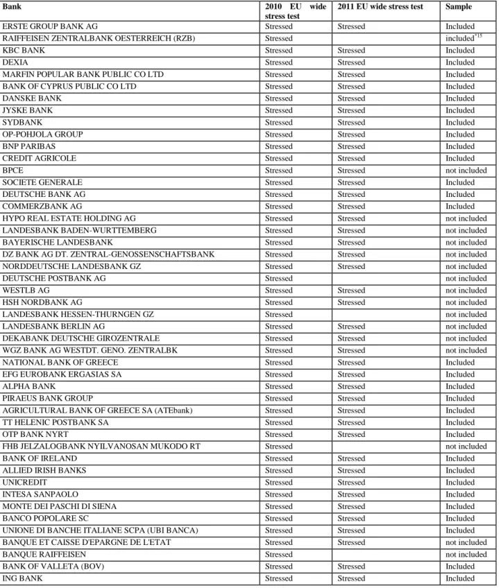
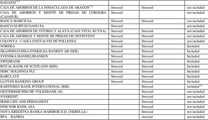
To select banks to integrate the sample, two criteria were identified. Firstly, following Cardinalli and Nordmark (2011), only banks that were stressed in both exercises are considered. This criterion led to an exclusion of the following banks: Deutsche Postbank AG, Landesbank Hessen-Thurngen GZ, FHB Jelzalogbank Nyilvanosan Mukodo RT, Bank Raiffesen, 11 spanish banks known as CAJAS, Banco Guipuzcoano SA, Oesterreichische Volksbank AG, Nykredit, Irish Life and Permanent, DNB Nor Bank ASA, Nova Kreditna Banka Maribor d.d. and BFA – Bankia. The next step is to exclude all banks not listed, or not traded on main national indices. This resulted in 50 banks being excluded. The final sample is therefore composed by 49 banks, as shown in the appendix. Following Campbell, Cowan and Salotti (2009), we use the Thomson Reuteurs DataStream daily price type P, which is the price already adjusted for stock splits and other capital events.
The length for estimation window in both exercises is different. The estimation period for the 2010 stress tests begins in 21 July, 2009, and ends in 21 July, 2010; for the 2011 stress tests the estimation period begins in 13 July, 2010, and goes to 13 July, 2011. The reason for that is explained later in the estimation procedure.
Theoretically, the market variable should represent all assets, regardless of being traded or untraded, as well as human capital which is commonly designated as “true market”; since that variable is unobservable, a market proxy is needed. Fama (1992) refers that a proxy for the market should be well diversified, like S&P CNX 500. In fact, S&P 500 and MSCI World stock indexes are two of the most important indexes selected as proxies for the market. The choice fell on MSCI World index, since this study focus on European banks and the MSCI World stock index has a more global perspective, covering over 6.000 securities in 24 developed markets countries. Cardinali and
12
Nordback (2011) also used the same index in their study. Values were also obtained from Thomson Reuters DataStream.
For individual volatility tests, the analysis focuses on the 5 banks with the worst results and the 5 banks with the best results. Given that it is not possible to match all chosen banks in both exercises, the sample was extended to 24 banks – 12 in the bottom and 12 in the top. Among these, banks that registered a good or bad result in both exercises to allow comparison were selected. Also two special cases were included, the Allied Irish Banks Plc which registered a low result in 2010 and a good one in 2011 test. A reverse result had the Greek TT Helenic Postbank S.A. which is also included. The final sample includes 18 banks – 8 with the best results, 8 with the worst results, and the two special cases referred above. To analyze the 2010 stress test results we use a sample data from 25-06-2010 to 20-08-2010, which led to 20 pre-observations and 20 post-observations, excluding the return of 23 July 2010. For 2011, the stress test results used begun in 17-06-2011 and ended in 12-08-2011; we also exclude the return of 15 July 2011. The remaining criteria expressed before applies.
Normal and abnormal returns
Event studies measure market reaction based on abnormal returns. If an event has market impacts, then abnormal returns should reflect it. The return of a security i for a time period t can be decomposed as follows:
I
where is the expected return of security i at time period t given by a certain model and is an error reflecting the unexpected variation in , reflected in the difference between the observed and expected return.
There are two different methods to compute returns: continuously compounded returns (logarithmic returns) or discrete returns (arithmetic returns). Logarithmic or log returns are widely used, since they reduce the risk of nonstationary problems. Nevertheless, log returns have a disadvantage when computing simple returns at a portfolio level,
i it
it R e
13
because . In his study, Fama (1976, pp 17-20) suggests
that continuously compounded returns conform better to the normality assumptions underlying regression. Thompson (1988 p. 81) reports that “return form also does not seem to be an important consideration in event studies”. Brown and Warner (1985), although using arithmetic returns, indicate that they get similar results using either simple or continuously returns. In this study, we consider continuously compounded returns, given that a large part of event studies does so. Therefore, the observed compounded return for bank i at day t may be expressed as follows
II
Where is the official current closing price of bank i at time t and is the last official closing price of bank i at time t-1.
Next, we try to understand how to deal with missing returns. Two methods could be used, namely, the “trade-to-trade” method and the “lumped returns” procedure. The first method only calculates returns from non-missing price days and treats returns on a missing price as missing. The lumped returns procedure consists on a trade-to-trade method for non-missing days, treating as zero returns the missing price days. Campbell, Cowan and Salotti (2009) refer that both methods produce similar performances. This paper uses lumped returns because it increases the number of observations, which can improve the efficiency of estimators and test statistics used in the event study (Maynes and Rumsey, 1993). Also, since we are studying different banks from different markets, using the trade-to-trade method would not allow us to match all observations across banks.
Stock prices are kept at local currency. Usually, to test stock price reactions there is no need to convert stock prices into a common currency (Campbell, Cowan and Salotti, 2009). 1 , , t i t i it P P Ln R
14
In order to compute normal returns or expected returns for each individual stock, we use a market model regression3
where is the rate of return of a market index on day t and is a zero-mean error
term with constant variance not correlated with , and not auto correlated.
So, the expected return is given by:
where and are ordinary least squares (OLS) estimates of and for each individual bank i.
Therefore, abnormal returns (AR) for each individual bank i at time t can be determined as
We could analyse each bank individually, but this would not be very informative because stock price reactions are also caused by other information unrelated to the event (global or individual news). Usually, daily excess returns are highly non-normal. Nevertheless, there is evidence that the mean excess return in a cross-sectional analysis of securities converges to normality, as the number of sample of securities increases (Brown and Warner, 1985). Despite that, they also refer that non-normality of daily returns has no obvious impact on event study methodologies. The information extracted by averaging abnormal returns becomes more reliable, since the information unrelated to the event should cancel out on average (de Jong, 2007). The equally-weighted cross-sectional average abnormal returns for a sample of w stocks for a time t is
To assess the impact of an event in the three days length as a whole, we need a time-series aggregation. The most common method used is the cumulative average abnormal returns (CAAR) that uses the sum of each daily average abnormal performance as the
3
15
abnormal performance measure. The CAAR starting at time through time (i.e.,
horizon length L = - +1) is defined as (Khotari and Warner, 2006):
Estimation procedure
Market model parameters and are usually estimated over a specific estimation window. There is no consensus, however, in literature regarding the length that should be used to estimate market model parameters. Brown and Warner (1980) use a 35-month period, but Fama et al (1969) use an estimation window of 24 35-months. Mikkelson and Partsch, (1986) used an estimation period of 140 trading days. Campbell et al (1997), suggest that if daily data is used the parameters of the market model could be estimated over a 120 days prior to event.
This paper follows Peristini et al (2010), that use one year daily data, but with a slight difference. Peristini et al (2010) use the same estimation period for three different events, with a gap time between them lesser than 3 months. The events in this study have a gap time of almost a year. This means that using the same estimation period (ending right before the first event) would minimize the regression’s power to explain 2011 EU-wide stress test disclosure, compared to 2010 EU-wide stress test disclosure. Thus, we use two different estimation periods in order to achieve more actual data for each event in study, leading to a better power explanation in both cases. Therefore, for the 2010 stress test results the parameters are based on a sample period from 21 July, 2009, to 21 July, 2010; this results in 262 observations for each individual bank. The 2011 market model parameters are based on an estimation window of also 262 observations, from 13 July, 2010, to 13 July, 2011, for each bank.
Testing procedure
Typically in event studies, statistical tests are based on the null hypothesis that mean abnormal return is equal to zero.
16
The null hypothesis to be tested for an individual day t is
against the alternative hypothesis:
The statistical tests usually adopted in the literature are divided into parametric tests and non-parametric tests.
Parametric tests are more often used in event studies. Nevertheless, non-parametric tests have been gaining importance in recent years, in response to a major criticism concerning parametric tests, which is that “they embody detailed assumptions about the probability distribution of returns” (Cowan, 1992, p.1). Another issue with parametric tests, as mentioned by Brown and Warner (1985), has to do with variance increases around the event date. In their opinion, this leads to a price reaction which actually does not happen more often than expected. Even so, if data assumptions are right, parametric tests will be the best option. The most common parametric tests used in event studies are the Patell (1976) standardized abnormal return, Brown and Warner (1985) with crude adjustment (CDA), and Boehmer, Musumeci and Poulsen’s (1991) standardized cross-sectional test. Non-parametric test are Corrado (1989) rank test and Cowan (1992) generalized sign test.
The test statistic for an individual day under the event window used in this paper follows Brown and Warner (1985), which reports a simple t-test,
where is the average abnormal return at day t and is the standard deviation at a
portfolio level at day t. AAR is assumed to be independent and identically distributed. Usually when the event day is the same for a sample of firms we cannot assume independence of abnormal returns. In order to assess independence of AAR, we perform
a Durbin-Watson test4 which tests for the first order serial independence. Nevertheless,
the standard deviation estimated using portfolio time series data from the estimation window automatically reflects all the pair wise correlations between abnormal returns,
4
17
thereby addressing cross-sectional dependence (Campbell, Cowan, and Salotti, 2009).
So, can be obtained as follows
- -
-
Since under the central limit theorem test statistic, we assume a standardized normal distribution
To test the event window as a whole, we need to compute the .The
hypotheses are:
-
-
The variance of cumulative average abnormal returns can be obtained through:
- - -
and the statistical test is given by:
-
-
As previously referred, non-parametric tests have been more used in event studies. However, researchers commonly use them to support their conclusions from parametric tests. For instance, the generalized sign test is commonly used to assess if conclusions from parametric tests are not affected by extreme observations.
In order to do that, this paper also performed the generalized sign test introduced by Cowan (1992).
18
“The generalized sign test compares the proportion of positive abnormal returns around an event to the proportion from a period unaffected by the event”. Cowan (1992, p.1). The null and the alternative hypotheses are given by:
-
-
The statistical test is based on a Binomial Distribution with a parameter p which is the fraction of positive abnormal returns over the estimation period. The estimate is computed as follows: where
n is the number of observations in estimation window and b is the number of stocks. The generalized sign test statistic will be
-
-
where w is the number of stocks in the event window for which the cumulative abnormal return is positive. The test statistic uses the normal approximation to the binomial distribution as expressed below,
-
In order to assess equality of variances in different samples, or the homogeneity of variances, we can use either the Levene’s test or the Bartlett’s test. As the Levene’s test is less sensitive to departures from normality the choice fell on last one.
19
The test statistic is defined as:
- - - - where:
K is the number of different groups to which the samples belong, N is the total number of samples in the i group and Ni is the number of samples in the i group
-
- is the value of the j sample from the i group.
The test compares the variance before and after the disclosure of results. The null hypothesis is defined as:
against the alternative hypothesis:
is the variance of bank before the disclosure of the results, is the variance of bank after the disclosure.
The Levene test rejects the hypothesis that variances are equal if:
- -
where is the upper critical value of the F-distribution with k-1 and N-K degrees of freedom at a significance level of .
Possible biases
Event studies are vulnerable to several aspects that may lead to incorrect inferences, as well as incorrect conclusions. For instance, a sample that contains a high number of
20
thinly traded stocks is characterized by numerous zero and large non-zero returns, resulting in non-normal returns distributions (Cowan, 1996). Infrequently traded securities are more affected by nonsynchronous returns period, which could lead to biased and inconsistent ordinary least squares estimates, as demonstrated by Scholes and Williams (1977), and Dimson (1979). In this study, the majority of banks included in the sample are actively traded. Nevertheless, some researchers, as Jain (1986), suggest that in most cases it is not important to adjust for thin trading.
Another possible source of bias occurs when incorrect assumptions about the data are imposed. To avoid asymptotic results, it is common to assume jointly normal and temporally IID asset returns. Nevertheless, Cowan (1992) concludes that the generalized sign test does not require cross-sectional symmetry of the abnormal returns for correct specification. Warner (1980; 1985) demonstrates that a sign test assuming an excess median of zero may be misspecified. For this reason, the study focuses on the mean, CAAR, also addressed in Cowan’s simulations (1992).
The presence of variance increases on the event day is another issue that has to be considered in an event study. Brown and Warner (1995) report that event-related variance increases cause standard parametric tests to report a price reaction, where none actually exists more often than expected. Extreme observations, commonly defined as outliers, could also have great impact on inferences. Yaari et al (2009) study the outliers’ impact on OLS estimates for U.S pharmaceutical companies, concluding that the presence of outliers may lead to biased OLS estimates. According to Cowan (1992), the generalized sign test performed well even in the presence of a variance increase in the event date, as well as with extreme observations. Finally, aggregated returns are usually analyzed, assuming uncorrelated abnormal returns of individual firms. This is a reasonable assumption when we do not deal with clustered data. Since both event dates in the study do not overlap, the assumption is acceptable.
21
4. Empirical results
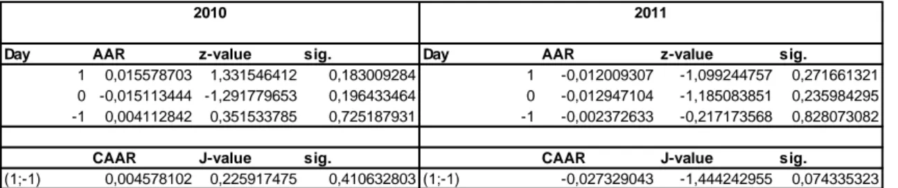
The table below shows the results of cumulative average abnormal returns (CAAR) and for Average Abnormal Returns (AAR), as well as their respective test statistic via the Brown and Warner (1989) method.
Table I. AAR and CAAR results and respective statistics in both exercises
The Table below presents the statistical results for CAAR using the generalized sign test.
Table II. GST results in both exercises and their respective statistics
The results around the 2010 disclosure are conclusive; none of the days has an AAR statistically significant. At the day prior to the disclosure of the results, we achieve a positive AAR, equal to 0,413%. The negative AAR of 1,5113% relative to the day of the event cannot be associated to results disclosure, given that they were only revealed after market closed.
The day after the release, which is a Monday, reveals a positive average abnormal return of 1,5579%, inverting the negative result of last trade day. This result may be associated with the fact that the market had sufficient time to analyze the results from stress test, responding positively to them. Looking into individual abnormal returns at day 1, it seems clear that the market remunerated banks in severe troubles but with good ratios. For instance, Bank of Cyprus had an abnormal return of 4,7085%, the Belgium Dexia had also a good AR of 7,1167% and also two Greek banks namely, Alpha Bank with 5,9267% and TT Hellenic with 14,0658%. This reveals that the market was able to distinguish between banks that needed and not needed capital raise, remunerating those
Day AAR z-value sig. Day AAR z-value sig.
1 0,015578703 1,331546412 0,183009284 1 -0,012009307 -1,099244757 0,271661321
0 -0,015113444 -1,291779653 0,196433464 0 -0,012947104 -1,185083851 0,235984295
-1 0,004112842 0,351533785 0,725187931 -1 -0,002372633 -0,217173568 0,828073082
CAAR J-value sig. CAAR J-value sig.
(1;-1) 0,004578102 0,225917475 0,410632803 (1;-1) -0,027329043 -1,444242955 0,074335323 2010 2011 2010 2011 CAAR 0,0045781 -0,027329 Zg 0,9997363 -3,9148746 sig 0,967124 0,0120266
22
expected to fail (or at least were expected to obtain a worse result), but that got good results. The positive cumulative average abnormal return of 0,4578% is also not statistically significant, leading us to not reject the hypothesis that the event impacted on markets. The GST rejected the null hypothesis of CAAR ≤ 0, indicating that the result is not derived from extreme observations.
The results from 2011 disclosure are not completely clarifying; once again, all AAR are statistically insignificant. Also, they were all negative. At the day prior to the event, the market reacted with a small loss of 0,2373%, but the next two trading days, the event day and the post-event day, registered bigger losses of 1,295% and 1,2%, respectively. This AAR indicates that the market was worried about the results, penalizing stock returns; this is a complete different situation than what occurred in the 2010 disclosure. The same exercise of observing individual abnormal returns was made, and the conclusions are not similar to the 2010 disclosure; 65% of banks registered losses. Surprisingly, banks with bad results and going through strong difficulties had positive and relevant abnormal returns, such as the Marfin Popular Bank Public Co Ltd, Bank of Ireland and 3 Greek banks. On the other hand, banks that registered good results (but worse than what they revealed in the previous test) were the most affected. This is the case of all Italian banks, two UK banks, and the French Societe Generale. This could be understood as a market response to the fact that this stress test was not conducted under an admissible adverse scenario. Looking for the whole three-day event window, it can be assumed an impact on markets, at the 10% significance level. Nevertheless, the fact that GST rejects null hypothesis corroborates the idea that the previous conclusion is due to extreme observations.
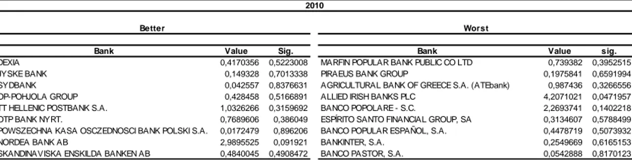
The Table below presents the results of Levene’s test to the selected banks.
Table III. Levene's results split into banks with good results (better) and banks with bad results (worst) in 2010 EU-wide stress tests
Bank Value Sig. Bank Value sig.
DEXIA 0,4170356 0,5223008 MARFIN POPULAR BANK PUBLIC CO LTD 0,739382 0,3952515
JYSKE BANK 0,149328 0,7013338 PIRAEUS BANK GROUP 0,1975841 0,6591994
SYDBANK 0,042557 0,8376631 AGRICULTURAL BANK OF GREECE S.A. (ATEbank) 0,987436 0,3266556
OP-POHJOLA GROUP 0,428458 0,5166891 ALLIED IRISH BANKS PLC 4,2071021 0,0471957
TT HELLENIC POSTBANK S.A. 1,0326266 0,3159692 BANCO POPOLARE - S.C. 2,2693741 0,1402218 OTP BANK NYRT. 0,7689606 0,386049 ESPÍRITO SANTO FINANCIAL GROUP, SA 0,3134607 0,5788499 POWSZECHNA KASA OSCZEDNOSCI BANK POLSKI S.A. 0,0172479 0,896206 BANCO POPULAR ESPAÑOL, S.A. 0,4478719 0,5073932
NORDEA BANK AB 2,9895525 0,091921 BANKINTER, S.A. 0,2549669 0,6165153
SKANDINAVISKA ENSKILDA BANKEN AB 0,4840045 0,4908472 BANCO PASTOR, S.A. 0,0542888 0,8170123
Worst Better
23
The results of banks with better ratios in the 2010 stress tests show that the perception of risk for these banks do not changed from the 20 days prior to the event, when compared to the 20 post event days. Only for Nordea Bank AB we can reject the null hypothesis of equal variances but only at 10% confidence level. These results make sense given that investors usually are more aware of possible losses or factors that may increase risk than the opposite. Looking for banks with worst results, a strange similar behavior compared with better banks may be highlighted. Again, only for one bank, the Allied Irish Banks PLC, we reject the hypothesis of equal variances between samples, although at the 5% significance level. As can be seen, for 7 banks we do not reject the null hypothesis belonging to the denominated PIIGS countries (Portugal, Italy, Ireland, Greece, and Spain). This result can be interpreted as a “vote of confidence” from the markets. For instance, in Greece the bailout was already approved, and for the other countries (except for Ireland) existed an expectation that the situation would improve.
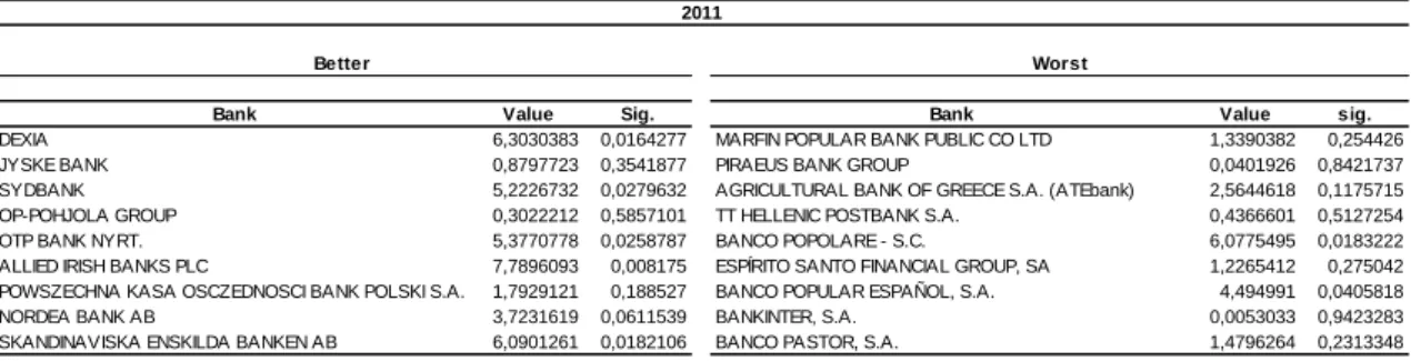
Table IV. Levene's results split into banks with good results (better) and banks with bad results (worst) in 2011 EU-wide stress tests
The results regarding 2011 were somewhat expected. Only two banks with worst ratio reject null hypothesis, the Banco Popolare SA and the Banco Popular Español SA, both at 5% significance level. Most of the impact on volatility occurred in banks with better results. Once again, for Nordea Bank the null hypothesis is rejected, but in this case the same applies to two other North banks. The fact that the null hypothesis is rejected for the Allied Irish Banks demonstrates how volatile its shares are. Dexia is other bank which has a rejected null hypothesis. This case was already expected, because, as
Bank Value Sig. Bank Value sig.
DEXIA 6,3030383 0,0164277 MARFIN POPULAR BANK PUBLIC CO LTD 1,3390382 0,254426
JYSKE BANK 0,8797723 0,3541877 PIRAEUS BANK GROUP 0,0401926 0,8421737
SYDBANK 5,2226732 0,0279632 AGRICULTURAL BANK OF GREECE S.A. (ATEbank) 2,5644618 0,1175715 OP-POHJOLA GROUP 0,3022212 0,5857101 TT HELLENIC POSTBANK S.A. 0,4366601 0,5127254
OTP BANK NYRT. 5,3770778 0,0258787 BANCO POPOLARE - S.C. 6,0775495 0,0183222
ALLIED IRISH BANKS PLC 7,7896093 0,008175 ESPÍRITO SANTO FINANCIAL GROUP, SA 1,2265412 0,275042 POWSZECHNA KASA OSCZEDNOSCI BANK POLSKI S.A. 1,7929121 0,188527 BANCO POPULAR ESPAÑOL, S.A. 4,494991 0,0405818
NORDEA BANK AB 3,7231619 0,0611539 BANKINTER, S.A. 0,0053033 0,9423283
SKANDINAVISKA ENSKILDA BANKEN AB 6,0901261 0,0182106 BANCO PASTOR, S.A. 1,4796264 0,2313348
2011
24
mentioned before, three months only after results were presented, Dexia needed a bailout. The other bank where the null is rejected is the OTP Bank.
25
5. Conclusion
Using standard event methods, this paper examines the impact of the following events on European banks stocks returns: the 2010 stress test results disclosure and the 2011 stress test results disclosure. Overall, tests suggest that both exercises were not very informative to the financial markets. Nevertheless, concerning 2011, results seem to show more reaction compared with the last exercise. Maybe this resulted from EBA’s effort to provide more and detailed information regarding banking entities and the stress test itself. The tests to individual volatility and the analysis to individual abnormal returns, provide indications that only specific banks were directly affected by the stress tests.
Therefore, the tests made in this paper suggest that no impact on market occurred directly from stress test results disclosure.
26
References
Balin, Brian J., 2008 Basel I, Basel II, and emerging markets: A nontechnical
analysis, Working papper, The Johns Hopkins University School of Advanced
International Studies, Washington DC
Boehmer, E., & Musumeci, J., & Poulsen, Annette B., 1991. Event-study methodology under conditions of event-induced variance, Journal of Financial Economics, 30 (2), 253-272.
Brown, S. J., & Warner. J. B. 1985. Using daily stock returns: The case of event studies.
Journal of Financial Economics 14, no. 1 (March): 3-31.
Campbell, C. J., & Cowan, A. R., & Salotti, V., 2009, Multi-country event study
methods, Working paper, Iowa State University
Campbell, J. Y., & Lo, A. W., & MacKinlay, A. C. 1997. The econometrics of
financial markets. Princeton, New Jersey: Princeton University Press.
Cardinali, A., & Nordmark J., 2011. How informative are bank stress tests? – Bank
opacity in the European union, Master Thesis in Finance, Lund University – School of
Economics and Management
Committee of European Banking Supervisors, CEBS’s press release on the results of the 2010 EU-wide stress testing exercise,
http://www.eba.europa.eu/documents/10180/15938/CEBSPressReleasev2.pdf/4a5b185f -43bf-4e4d-b1de-c50c7e656b87, published at July 23, 2010
Committee of European Banking Supervisors, Aggregate outcome of the 2010 EU wide stress test exercise coordinated by CEBS in cooperation with the ECB, http://www.eba.europa.eu/documents/10180/15938/Summaryreport.pdf/95030af2-7b52-4530-afe1-f067a895d163, published at July 23, 2010
Committee of European Banking Supervisors, 2010 results,
http://www.eba.europa.eu/documents/10180/15938/Listofbanksv2.pdf/af7d6849-5882-4f83-82e7-b4ff9a63a112, published at July 23, 2010
Corrado, Charles J., 1989. A nonparametric test for abnormal security-price performance in event studies, Journal of Financial Economics, 23, 385–95.
Cowan, Arnold R. 1992 - Non parametric event study tests, Review of Quantitative
Finance and Accounting 2 (December 1992): 343-358
Cowan, Arnold R. and Anne M. A. Sergeant, 1996. Trading frequency and event study test specification, Journal of Banking and Finance, 20(10, Dec), 1731–1757.
27
de Jong, F., 2007. Event studies methodology. Tilburg University Available
at:http://www.tilburguniversity.edu/research/institutes-and-research-groups/center/staff/dejong/preprints/eventstudies.pdf,
Dimson, E., 1979. Risk measurement when shares are subject to infrequent trading,
Journal of Financial Economics 7, 197-226.
European Banking Authority, 2011 EU-wide stress-test Methodolological Note – Additional guidance:,
http://www.eba.europa.eu/documents/10180/15935/Additional+guidance+to+the+meth odological+note.pdf/db1da102-7669-41eb-a9e9-3f44c23610ef, published at June 9, 2011
European Banking Authority, Results of the 2011 EU-wide stress test,
http://www.eba.europa.eu/documents/10180/15935/2011+EU- wide+stress+test+results+-+press+release+-+FINAL.pdf/b8211d3b-562e-40d4-80f8-0b5736c20345, published at July 15, 2011
European Banking Authority, Opening Statement, Publication of the 2011 EU-wide
Stress Test Results, http://www.eba.europa.eu/documents/ 10180/15935/ Opening
+statement+-+Andrea+Enria+-+FINAL.pdf/d0024654-e56a-4263-b587-3e691565dc3a ,published at July 15 ,2011
European Banking Authority, European Banking Authority 2011 EU-wide stress test - aggregate report,
http://www.eba.europa.eu/documents/10180/15935/EBA_ST_2011_Summary_Report_ v6.pdf/54a9ec8e-3a44-449f-9a5f-e820cc2c2f0a, published at July 15 ,2011
European Banking Authority, CT1 ratios under the adverse scenario,
http://www.eba.europa.eu/documents/10180/15935/Summary+of+CT1+ratios+under+th e+adverse+scenario.pdf/986761b3-0a69-40fc-a92d-a651fe074505, published at June 15, 2011
Fama, E.F.,& Fisher, L.,& Jensen, M.C. & Roll, R., 1969. The adjustment of stock prices to new information. International Economic Review, 10(1), pp. 1-21.
Fama, Eugene F.,1976, Foundations of finance. New York: Basic Books, Inc.,
Fama, E.F., & French, K.R., 1992. The cross section of expected stock returns. Journal
of Finance 47, 427-465
Haggard, K. S., & Howe. J.S. 2007. Are banks opaque. Working Paper, University of Missouri.
Hirtle, B, & Lopez. J. 1999. Supervisory information and the frequency of bank examinations. Federal Reserve Bank of New York Economic Policy Review 5, no. 1 (April): 1-19.
28
Iannotta, G. 2006. Testing for opaqueness in the European banking industry: Evidence from bond credit ratings. Journal of Financial Services Research 30, no. 3 (December): 287-309.
Jain, P.C., 1986. Analysis of the distribution of security market model prediction errors for daily returns data. Journal of Accounting Research, 24(1), pp. 76-96.
Jones, J. S., & Lee, W. Y. & Yeager, T. J., 2011. Opaque banks, price discovery, and
financial instability. Working paper, Drury University – Breech School of Business
Maynes, E. & Rumsey, J. 1993. Conducting event studies with thinly traded stocks,
Journal of Banking and Finance 17, 145–157.
Mikkelson, Wayne H. & Partch, M. Megan 1986. Valuation effects of security offerings and the issuance process, Journal of Financial Economics 15, 31–60.
Morgan, D.P., 2002. Rating banks: Risk and uncertainty in an opaque industry. American Economic Review 92, no. 4 (September): 874-88.
Patell, James M., 1976. Corporate forecasts of earnings per share and stock price behavior: Empirical tests, Journal of Accounting Research 14, 246–276.
Peristiani, S.,& Morgan, D.P. & Savino, V., 2010. The information value of the stress
test and bank opacity. Federal Reserve Bank of New York Staff Reports, no. 460.
Available at: http://www.ny.frb.org/research/staff_reports/sr460.pdf, published at July 2010
Khotari, S.P., & Warner, J. B., 2006. Econometrics of event studies, Working papper, Massachusetts Institute of Technology (MIT) - Sloan School of Management, Cambridge
Scholes, M., & Williams J. T. 1977. Estimating betas from non-synchronous trading.
Journal of Financial Economics 5, 309-327.
Thompson, Joel E., 1988, More methods that make little difference in event studies,
Journal of Business Finance and Accounting, 15: 77-86
Yaari U., & Theodossiou A. K., & Theodossiou P., 2009 Beta estimation with stock
29
APPENDIX
Regulatory framework Basel I
In 1970s the world was facing serious disturbances in international currency and banking markets, which had in 1974 its highest expression with Bankhaus Hersttat´s collapse. In order to harmonize banking standards and regulations within and between member states, G-10 countries plus Spain at the Bank of International Settlement (BIS) formed a standing committee called Basel Committee of Banking Supervision (BCBS), also known as Basel Committee (Balin 2008).
The International Convergence of Capital Measurements and Capital Standards released in July of 1988, also referred as Basel I, published by BCBS had the intention to promote harmonization of regulatory and capital adequacy standards across Basel Committee members. An important point to note is that Basel I cares about adequate capital against credit risk and not for other risk factors such as currency risk, interest rates changes or macroeconomic downturns. It implemented a credit risk measurement framework with a minimum capital standard of 8% by end-1992. As referred by Balin (2008) the accord is divided into four “Pillars”:
First Pillar (The constituents of capital) – defines what types of on-hand capital are counted as a bank´s reserves and how much of each type of reserve capital a bank can hold. The “eligible capital” is divided into 2 Tiers.
Tier 1 Capital – includes disclosed capital reserves and other capital paid for by the sale of bank equity (namely, stock and preferred shares); Tier 2 Capital – include reserves created to cover potential loan losses, holdings of subordinated debt, hybrid debt/equity instruments holdings, and potential gains from the sale of assets purchased through the sale of bank stock.
Basel Accord defines that banks must hold the same amount of which one:
30
Second Pillar (Risk Weighting) – the second Pillar says how banks must weight their assets according to risk. It divides into five risk categories all assets on a bank´s balance sheet. Assets like cash held by banks or sovereign debt are allocated in first category and weighted at 0% (considerate “riskless” assets). Second category weights assets at 20% which includes for instance multilateral development bank debt, third at 50% which is the case of residential mortgages and fourth at 100% we have equity assets or Eurobonds. The fifth category encompasses claims on domestic public sector entities, which can be valued at 0, 10, 20 or 50% depending on the central bank´s description.
Third Pillar (Target standard ratio): defines that at least 8% of bank ´s risk-weighted assets must be covered by Tier 1 and Tier 2 capital reserves, where 4% must be covered by Tier 1 capital.
Fourth Pillar (Transitional and Implementing Agreements): set to insure that Basel Accord is followed.
Four primary sources of criticisms were pointed out to Basel I (Balin 2008). First source considered is what he calls “omissions” because the Accord only covers credit risk and only targets G-10 members and does not have ability to influence counties omitting market discipline. Secondly, points to the way that the Accord was implemented. The third group of criticisms has to do with the ability of banks to risk-weight assets in a way more convenient to them. Finally, is hard to implement in emergent markets even if was never intent.
31
Basel II
After the introduction of market risk with the Market Risk Amendment (1996) and the publication of Settlement Risk – Continuous linked Settlement CLS (2002), was released in 2004 the New Basel Capital Accord, formally known as A Revised Framework on International Convergence of Capital Standards and informally as Basel II. This new capital requirements accord consists of three pillars, and is to be applied on a consolidated basis to internationally active banks:
The First Pillar – Minimum Capital Requirements
The Second Pillar – Supervisory Review Process
The Third Pillar – Market Discipline
The first pillar considers 3 main sources of risk: credit risk, operational risk and market risk.
For credit risk, banks have a possibility to choose between three different approaches, a Simplified Standardized Approach (SSA) based on ratings of the external credit assessment institutions, a Foundation Internal Rating Based (FIRB) or an Advanced Internal Rating Based (AIRB). These two last ones are similar based on Probability of Default (PD), Loss given Default (LGD) and Exposure at Default (EAD) but in first case LGD and EAD will depend on fixed weights approved by national supervisors and in second case banks may use their own estimates.
Operational risk considers riskiness related to internal processes, systems and people can be measured by Basic Indicator Approach (BIA), Standardized Approach (SA) and Advanced Measurement Approach.
In market risk are considered losses due to changes in asset prices. In this evaluation of risk is made a distinction between fixed income and products such as equity, commodity and foreign exchange vehicles and also a separation of the two principal risks that contributes to the market risk: interest rate and volatility risk (Balin, 2008). To measure this kind of risk a several methodologies are able such as Value-at-risk (VaR), The Simplified Approach, scenario analysis and Internal Model Approach. VaR is considered the best option.
32
Once computed the 8% requirement for credit-default capital adequacy and reserves needed to guard against operational and market risk, banks can achieve “total capital adequacy”.
Basel II sets capital ratio must be no lower than 8% using the definition of regulatory capital and risk-weighted assets and Tier 2 is limited to 100% of Tier 1 (BCBS, 2004). The capital definition was expanded into three tiers.
Tier 1 (Core Capital): composed by disclosed reserves and issued and fully paid ordinary shares/common stock and non-cumulative perpetual preferred stock. Tier 2 (Supplementary Capital): under this classification are undisclosed reserves, revaluation reserves, general provisions/general loan-loss reserves, hybrid debt capital instruments and subordinated term debt.
Tier 3 (sub-supplementary Capital): subordinated debt with maturity at issue of 2 to 5 years.
To meet Market Risk Charge (MRC) introduced by the 1996 Market Risk Amendment, banks are able to use all 3 tiers of capital with the following restriction:
The main goal of Supervisory Review Process is to ensure that banks are able to manage their risks beyond the core minimum requirements, given to supervisory more responsibility to evaluate the models used by banks for the calculation of risks and capital requirements. The main risks under Pillar 2 are for instance credit concentration risk, interest rate risk in banking book, business and strategic risk, business cycle effects (Ahmed and Khalidi, 2007).
According BCBS, the main purpose of Pillar III is to complement the Minimum Capital Requirements and Supervisory Review Process and keep general public fully inform regarding bank´s capital and risk-taking positions.
33
Table V. List of stressed banks and identification of which were included in the portfolio
Bank 2010 EU wide
stress test
2011 EU wide stress test Sample
ERSTE GROUP BANK AG Stressed Stressed Included
RAIFFEISEN ZENTRALBANK OESTERREICH (RZB) Stressed included*15
KBC BANK Stressed Stressed Included
DEXIA Stressed Stressed Included
MARFIN POPULAR BANK PUBLIC CO LTD Stressed Stressed Included
BANK OF CYPRUS PUBLIC CO LTD Stressed Stressed Included
DANSKE BANK Stressed Stressed Included
JYSKE BANK Stressed Stressed Included
SYDBANK Stressed Stressed Included
OP-POHJOLA GROUP Stressed Stressed Included
BNP PARIBAS Stressed Stressed Included
CREDIT AGRICOLE Stressed Stressed Included
BPCE Stressed Stressed not included
SOCIETE GENERALE Stressed Stressed Included
DEUTSCHE BANK AG Stressed Stressed Included
COMMERZBANK AG Stressed Stressed Included
HYPO REAL ESTATE HOLDING AG Stressed Stressed not included
LANDESBANK BADEN-WURTTEMBERG Stressed Stressed not included
BAYERISCHE LANDESBANK Stressed Stressed not included
DZ BANK AG DT. ZENTRAL-GENOSSENSCHAFTSBANK Stressed Stressed not included
NORDDEUTSCHE LANDESBANK GZ Stressed Stressed not included
DEUTSCHE POSTBANK AG Stressed not included
WESTLB AG Stressed Stressed not included
HSH NORDBANK AG Stressed Stressed not included
LANDESBANK HESSEN-THURNGEN GZ Stressed not included
LANDESBANK BERLIN AG Stressed Stressed not included
DEKABANK DEUTSCHE GIROZENTRALE Stressed Stressed not included
WGZ BANK AG WESTDT. GENO. ZENTRALBK Stressed Stressed not included
NATIONAL BANK OF GREECE Stressed Stressed Included
EFG EUROBANK ERGASIAS SA Stressed Stressed Included
ALPHA BANK Stressed Stressed Included
PIRAEUS BANK GROUP Stressed Stressed Included
AGRICULTURAL BANK OF GREECE SA (ATEbank) Stressed Stressed Included
TT HELENIC POSTBANK SA Stressed Stressed Included
OTP BANK NYRT Stressed Stressed Included
FHB JELZALOGBANK NYILVANOSAN MUKODO RT Stressed not included
BANK OF IRELAND Stressed Stressed Included
ALLIED IRISH BANKS Stressed Stressed Included
UNICREDIT Stressed Stressed Included
INTESA SANPAOLO Stressed Stressed Included
MONTE DEI PASCHI DI SIENA Stressed Stressed Included
BANCO POPOLARE SC Stressed Stressed Included
UNIONE DI BANCHE ITALIANE SCPA (UBI BANCA) Stressed Stressed Included
BANQUE ET CAISSE D'EPARGNE DE L'ETAT Stressed Stressed not included
BANQUE RAIFFEISEN Stressed not included
BANK OF VALLETA (BOV) Stressed Stressed Included