Cardiac motion and deformation estimation in tagged magnetic resonance imaging

Declaração

Nome: Pedro André Gonçalves Morais

Endereço electrónico: a57113@alunos.uminho.pt Telefone: (+351) 916077002

Número do Cartão de Cidadão: 13715779

Título da dissertação:

Cardiac Motion and Deformation estimation in tagged Magnetic Resonance Imaging Estudo do movimento e deformação cardíaca em imagens de ressonância magnética marcadas.

Orientadores:

Professor Doutor Jaime Francisco Cruz Fonseca Professor Doutor Jan D’hooge

Ano de conclusão: 2013

Designação do Mestrado: Mestrado Integrado em Engenharia Biomédica Área de Especialização: Electrónica Médica

Escola: de Engenharia

É AUTORIZADA A REPRODUÇÃO PARCIAL DESTA TESE, APENAS PARA EFEITOS DE INVESTIGAÇÃO, MEDIANTE DECLARAÇÃO

ESCRITA DO INTERESSADO, QUE A TAL SE COMPROMETE.

Universidade do Minho, ____/____/____

iii À Ana Silva, que te sirva de inspiração:

v

Acknowledgements/Agradecimentos

This master thesis symbolizes the end of a cycle, where important intellectual and life experiences contributed to the final definition of my own identity. After these 5 years, in the amazing city of Braga, together with wonderful persons that always helped me, I am ready to start a new journey with more experience and self-knowledge. Starting from today, I want to show the best of me, without the fears of the past.

First of all, I want to thank Professor Jan D’hooge, the promoter of the current thesis. All your interest during the last year was amazing, and your opinions during the meetings were essential to improve the final work. During the thesis, I always felt your support, even when I returned to Portugal. I expect to keep our collaborations in future works, and I expect in a future PhD project. I also want to thank Piet Claus for the collaboration in image analysis and support about the clinical relevance of the results.

I need to thank my daily supervisor, Brecht Heyde, for all the support, ideas, and discussions to improve the final work. The new proposed methodologies were impossible without your experience. You have helped me to grow in the area of imaging processing, where, in my opinion, you are a reference.

Ao professor Jaime Fonseca, tenho de agradecer pelo apoio que obtive para manter o projecto que iniciei em Leuven, assim como por todas as opiniões durante a elaboração do mesmo. Agradeço também pela total disponibilidade durante a tese.

Para o Daniel Barbosa, tenho de te agradecer por todas as reuniões, por todo o

feedback que obtive e suporte na elaboração da tese. Eu também vejo em ti uma

referência na área, um modelo a seguir. Tenho também de agradecer a ti e à Dalila Roupar, por todo o apoio extra tese, durante e após o ERASMUS.

Ao professor João Vilaça, tenho que agradecer pela oportunidade que me deu de entrar no mundo da investigação antes da minha tese. Agradeço por toda a colaboração durante a realização desta tese, por todas as discussões, formas de validação, métodos para apresentação dos temas da tese e por todo o equipamento que me disponibilizou.

Ao Sandro Queirós, tenho que agradecer por todo o acompanhamento na tese e pela amizade. Já trabalhamos juntos há muitos anos e espero continuar com esta ligação. As discussões que tivemos foram essenciais para desenvolver os métodos. Tenho também que agradecer aos restantes membros do gabinete: António Moreira, João Fonseca, João Spranger, Nuno Rodrigues, Mafalda Couto e Pedro Rodrigues.

vi

Agradeço também à Teresa Pinto pelo suporte na escrita da tese em inglês e à professora Ana Cristina Braga pelo apoio na análise estatística.

Tenho também que agradecer a toda a minha família, aos meus pais José Morais e Joaquina Gonçalves, irmão Jorge Morais, cunhada Catarina Moreira, avós, tios, primos e padrinhos por todo o apoio. Vocês são as pessoas que sempre estiveram presentes e que sempre quiseram que eu alcançasse todas as metas que ia traçando, sem nunca desistir. Todos vocês foram essenciais durante a elaboração desta tese de mestrado. Quero também agradecer à minha família académica, família Teixeira, com particular ênfase ao meu “afilhado” João Meireles e “netos” Francisco Lobo, Márcia Costa e Vitor Faria. Vocês são uma fonte de orgulho e de motivação, espero que daqui a alguns anos esteja a assistir às vossas dissertações e que consigam muito mais do que eu. Eu acredito no vosso valor e vão ter sempre o meu apoio em tudo.

À Cristiana Fernandes tenho que agradecer por todo o apoio durante a escrita da tese, por me teres acompanhado nos momentos em que me senti mais frágil psicologicamente, por todas as opiniões e imparcialidade. Foste a pessoa que me ajudou a crescer dizendo para desistir de viver num mundo que não existe e deixar de pensar em tudo ao detalhe, seguindo em frente. Se eu acabei esta tese, foi tudo graças a ti.

À Ana Silva, penso que a dedicatória inicial diz tudo. Tu foste a pessoa que marcou a mudança em mim. Quando uma pessoa sente-se perdida e não sabe o que mais fazer, receber um apoio como tu fizeste, provocou uma mudança tão grande em mim. Passaram tantos anos, e mesmo assim tu foste capaz de me apoiar quando eu mais precisei. Estes últimos meses foram tão desgastantes, não só para mim mas também para ti, mas encontrei em ti a fonte de suporte e motivação que precisava para terminar tudo. Espero que em breve, também consiga ver-te a terminar tudo. Nunca desistas.

Por fim, existe um último agradecimento que quero fazer. Quero agradecer a quem me ajudou a elaborar todos os métodos e os vários resultados apresentados. Agradeço à pessoa que me dizia “eu sei que vais conseguir, porque sei o enorme valor

que tens”. Todos os métodos aqui propostos não são só meus, mas também de quem me

apoiou a este ponto. Todas as linhas presentes na tese foram feitas com o teu apoio. Um dia gostava de poder colocar aqui o teu nome, porque em parte, esta tese também é tua.

Thank you. Dank u wel. Obrigado a todos,

Pedro Morais

vii

Summary

Cardiovascular diseases are the main cause of death in Europe, with an estimate of 4.3 million deaths each year. The assessment of the regional wall deformation is a relevant clinical indicator, and can be used to detect several cardiac lesions. Nowadays, this study can be performed using several image modalities. In the current thesis, we focus on tagged Magnetic Resonance imaging (t-MRI) technique. Such technique allows acquiring images with tags on the myocardium, which deform with the muscle.

The present thesis intends to assess the left ventricle (LV) deformation using radial and circumferential strain. To compute such strain values, both endo- and epicardial contours of the LV are required.

As such, a new framework to automatically assess the LV function is proposed. This framework presents: (i) an automatic segmentation technique, based on a tag suppression strategy followed by an active contour segmentation method, and (ii) a tracking approach to extract myocardial deformation, based on a non-rigid registration method. The automatic segmentation uses the B-spline Explicit Active Surface framework, which was previously applied in ultra-sound and cine-MRI images. In both cases, a real-time and accurate contour was achieved. Regarding the registration step, starting from a state-of-art approach, termed sequential 2D, we suggest a new method (termed sequential 2D+t), where the temporal information is included on the model.

The tracking methods were first tested on synthetic data to study the registration parameters influence. Furthermore, the proposed and original methods were applied on porcine data with myocardial ischemia. Both methods were able to detect dysfunctional regions. A comparison between the strain curve in the sequential 2D and sequential 2D+t strategies was also shown. As conclusion, a smoothing effect in the strain curve was detected in the sequential 2D+t strategy. The validation of the segmentation approach uses a human dataset. A comparison between the manual contour and the proposed segmentation method results was performed. The results, suggest that proposed method has an acceptable performance, removing the tedious task related with manual segmentation and the intra-observer variability. Finally, a comparison between the proposed framework and the currently available commercial software was performed. The commercial software results were obtained from core-lab analysis. An acceptable result (r = 0.601) was achieved when comparing the strain peak values. Importantly, the proposed framework appears to present a more acceptable result.

ix

Resumo

As doenças cardiovasculares são a principal causa de morte na Europa, com aproximadamente 4.7 milhões de mortes por ano. A avaliação da deformação do miocárdio a um nível local é um importante indicador clínico e pode ser usado para a deteção de lesões cardíacas. Este estudo é normalmente realizado usando várias modalidades de imagem médica. Nesta tese, a Resonância Magnética (RM) marcada foi a técnica selecionada. Estas imagens têm marcadores no músculo cardíaco, os quais se deformam com o miocárdio e podem ser usados para o estudo da deformação cardíaca.

Nesta tese, pretende-se estudar a deformação radial e circunferencial do ventrículo esquerdo (VE). Assim, um contorno do endo- e epicárdio no VE é essencial.

Desta forma, uma ferramenta para o estudo da deformação do VE foi desenvolvida. Esta possui: (i) um método de segmentação automático, usando uma estratégia de supressão dos marcadores, seguido de uma segmentação c um contorno ativo, e (ii) um método de tracking para determinação da deformação cardíaca, baseado em registo não rígido. A segmentação automática utiliza a ferramenta B-spline Explicit

Active Surface, que foi previamente aplicada em imagens de ultrassons e cine-RM. Em

ambos os casos, uma segmentação em tempo real e com elevada exatidão foi alcançada. Vários esquemas de registo foram apresentados. Neste ponto, começando com uma técnica do estado da arte (designada de sequencial 2D), uma nova metodologia foi proposta (sequencial 2D+t), onde a informação temporal é incorporada no modelo.

De forma a analisar a influência dos parâmetros do registo, estes foram estudados num dataset sintético. De seguida, os diferentes esquemas de registo foram testados num dataset suíno com isquemia. Ambos os métodos foram capazes de detetar as regiões disfuncionais. De igual forma, utilizando as curvas de deformação obtidas para cada um dos métodos propostos, foi possível observar uma suavização na direção temporal para o método sequencial 2D+t. Relativamente à segmentação, esta foi validada com um dataset humano. Um contorno manual foi comparado com o obtido pelo método proposto. Os resultados sugerem que a nova estratégia é aceitável, sendo mais rápida do que a realização de um contorno manual e eliminando a variabilidade entre observadores. Por fim, realizou-se uma comparação entre a ferramenta proposta e um software comercial (com análise de core-lab). A comparação entre os valores de pico da deformação exibe uma correlação plausível (r=0.601). Contudo, é importante notar, que a nova ferramenta tende a apresentar um resultado mais aceitável.

xi

Contents

Figures list ... xvii

Tables list ... xxiv

1. Introduction... 3

1.1. Cardiac anatomy and physiology ... 3

1.2. Cardiac motion ... 4

1.2.1. Cardiovascular diseases ... 4

1.2.2. Regional heart deformation ... 5

1.2.3. Tagged Magnetic Resonance Imaging ... 6

1.3. Medical Image Processing ... 10

1.3.1. Medical Image Segmentation ... 10

1.3.2. Medical Image Registration ... 12

1.4. Motivation ... 15

1.5. Aim ... 16

1.6. Thesis outline ... 17

2. LV tracking and segmentation in t-MRI images ... 21

2.1. LV tracking methods ... 21

2.2. LV segmentation methods ... 26

2.2.1. LV segmentation after un-tagging t-MRI images ... 26

2.2.2. LV segmentation on the original t-MRI image ... 29

2.3. Summary ... 30

3. Mathematical Background ... 33

xii 3.1.1. Transformation Model ... 33 3.1.2. Cost function ... 35 3.1.3. Similarity Metrics ... 35 3.1.4. Regularization Term ... 39 3.1.5. Optimization ... 39 3.1.6. Image interpolators ... 40

3.1.7. Traditional motion estimation scheme: sequential 2D FFD formulation 41 3.2. Image Segmentation ... 42

3.2.1. Active Contours ... 42

3.2.2. B-spline Explicit Active Surfaces ... 44

3.3. Improving the initialization: template matching ... 46

3.4. Application: the BEAS threshold algorithm ... 47

3.5. Evaluating image segmentation quality ... 48

3.6. Strain estimation ... 49

4. Methodology ... 55

4.1. Overview ... 55

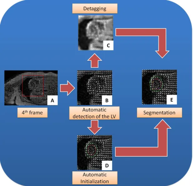
4.2. Automatic myocardial segmentation ... 55

4.2.1. Overview ... 55

4.2.2. Automatic detection of the LV ... 57

4.2.3. Image detagging ... 59

4.2.4. Automatic Initialization ... 63

4.2.5. Segmentation propagation ... 66

4.3. Cardiac Motion estimation ... 67

4.3.1. Sequential 2D+t FFD formulation ... 67

4.3.2. Fixed 2D+t FFD formulation ... 69

xiii 4.4.1. Strain estimation in the sequential 2D+t and fixed 2D+t FFD formulation 70

4.4.2. Contours definition on the ED frame ... 70

5. Methods ... 75

5.1. Datasets ... 75

5.2. Experiments ... 77

5.2.1. Parameter tuning ... 77

5.2.2. Detection of (dys)functional regions ... 77

5.2.3. Validation of the (semi-) automatic segmentation approach ... 77

5.2.4. Validation of the proposed sequential 2D+t FFD formulation ... 78

5.2.5. Comparison of the proposed algorithm with a commercial state-of-the art solution 79 6. Results ... 83

6.1. Parameter tuning ... 83

6.2. Detection of (dys)functional regions ... 86

6.3. Validation of the (semi-) automatic segmentation approach ... 88

6.4. Validation of the proposed sequential 2D+t FFD formulation ... 89

6.5. Comparison of the proposed algorithm with a commercial state-of-the art solution 91 7. Discussion ... 99

7.1. Parameter tuning ... 99

7.2. Detection of (dys)functional regions ... 100

7.3. Validation of the (semi-) automatic segmentation approach ... 101

7.4. Validation of the proposed sequential 2D+t FFD formulation ... 102

7.5. Comparison of the proposed algorithm with a commercial state-of-the art solution 104 8. Conclusions and contributions ... 111

xiv

8.2 Contributions ... 112

9. References... 117

10. Appendix I – Details about the automatic segmentation method ... 127

11. Appendix II – Number of correction in the automatic contour ... 129

12. Appendix III – LV tracking and segmentation results ... 130

13. Appendix IV – Validation of the proposed sequential 2D+t FFD formulation using a published result ... 132

14. Appendix V – Global strain curve obtained in proposed framework and in commercial software... 133

15. Appendix VI – Results obtained in each slice for the proposed framework and commercial software ... 134

16. Appendix VII – Validation of the proposed framework using the commercial software results as ground truth ... 137

xv

Abbreviations

2D two-dimensional

2D+t two-dimensional plus time 3D three-dimensional

4D four-dimensional

APD average perpendicular distance

BE bending energy

BEAS B-spline Explicit Active Surfaces CHDs Coronary Heart Diseases

CSPAMM Complementary spatial modulization of magnetization

CT Computed Tomography

CVDs Cardiovascular Diseases

DANTE Delays alternating with nutations for tailored excitations DE-MRI delay-enhancement Magnetic Resonance Imaging DICOM Digital Imaging and communication in Medicine

DOF Degrees of freedom

ECG electrocardiogram

ED end-diastole

EES Error at end-systole

ES end-systole

FFD free form deformation FFT Fast Fourier Transform

HARP Harmonic phase

ITK Insight Segmentation and Registration Toolkit

LA long-axis

LBFGSB limited memory Broyden Fletcher Goldforb Shannon LOA limits of agreement

LV left ventricle

MR Magnetic Resonance

MRI Magnetic Resonance Imaging

MI Mutual Information

MMI Mattes Mutual Information NMI Normalized Mutual Information NRR Non-Rigid Registration

NURBS NonUniform Rational B-splines PCA Principal Component Analysis PET Positron Emission Tomography

RF Radio-frequency

RMSE Root mean square error ROI region of interest

RV right ventricle

SA short-axis

SM Similarity Metric

SNR Signal Noise Ratio

xvi

SPECT Single Photon Emission Computed Tomography SSD sum of squared differences

SSFP Steady-State Free Precession

t-MRI tagged Magnetic Resonance Imaging TPF true positive fraction

US ultrasound

xvii

Figures list

Figure 1.1 - The heart anatomy. Adapted from [6]. ... 3

Figure 1.2 – Distribution of the blood output from the LV [2]. ... 4

Figure 1.3 - Five t-MRI sequences. ... 7

Figure 1.4 - Schematic about the SPAMM tagging pulse methodology. Adapted from [26]. ... 9

Figure 1.5 - Definition of the SA and LA views. Adapted from [28]. ... 9

Figure 1.6 - 3D tagging structure visualized by isosurface rendering of the 3D dataset [29]. ... 10

Figure 1.7 - 3D endocardium segmentation in echocardiography image [44]. ... 11

Figure 1.8 – Registration problem. Searching for the best transformation (T) capable to map the moving image on the fixed image with minimum error. ... 12

Figure 1.9 - Registration problem scheme... 13

Figure 1.10 – Transformation models used by (a) rigid registration, (b) affine registration, and, (c) non-rigid registration [46]. ... 13

Figure 1.11 - Example of thorax tumor staging from PET and CT [46]. ... 14

Figure 1.12 - Example of fusion data from MR and CT by image registration. (left) MR overlaid on CT and (right) CT overlaid on MR [46]. ... 14

Figure 1.13 - (a) Deaths by cause in Europe (b) Death rates from cardiovascular problem in each country of Europe [48]. ... 15

Figure 2.1 - Block scheme of strain estimation using tracking landmarks... 22

Figure 2.2 - Block scheme of strain estimation using HARP. ... 23

Figure 2.3 - Block scheme of strain estimation using gabor filter bank. ... 23

Figure 2.4 - Block scheme of strain estimation using deformable models... 24

Figure 2.5 - Block scheme of strain estimation using optical flow methodology. ... 24

Figure 2.6 - Block scheme of strain estimation using non-rigid registration. ... 24

Figure 2.7 - Different registrations schemes: a) pairwise 2D [68], (b) fixed 2D+t alignment [70], (c) joint 2D+t alignment [10]. ... 25

Figure 2.8 - Methods to segment t-MRI images. ... 26

Figure 2.9 - Block scheme for segmentation in t-MRI using the strategy proposed in [76]. ... 27

Figure 2.10 - Block scheme for segmentation in t-MRI using the strategy proposed in [77]. ... 28

xviii

Figure 2.11 - Block scheme for segmentation in t-MRI using the strategy proposed in [78]. ... 28 Figure 2.12 - Block scheme for segmentation in t-MRI using the strategy proposed in [83]. ... 29 Figure 2.13 - Block scheme for segmentation in t-MRI using the strategy proposed in [89]. ... 29 Figure 2.14 - Block scheme for segmentation in t-MRI using the strategy proposed in [80]. ... 30 Figure 2.15 - Block scheme for segmentation in t-MRI using the strategy proposed in [75]. ... 30 Figure 3.1 - The basic components of the registration framework. ... 33 Figure 3.2- B-spline mesh overlaid over the reference image. The transformation parameters are only defined on the mesh knot [47]... 34 Figure 3.3 - Conceptual representation of the multi-resolution registration process [85]. ... 35 Figure 3.4 - Binary synthetic image. The black squares represent 0, and the white represent 1... 36 Figure 3.5 - Joint histogram used in a registration problem between a CT and MR example [87]. ... 37 Figure 3.6 - Parzen Window (blue), constructed by superimposing kernel functions centered on the samples of the image [85]. ... 38 Figure 3.7 - Regularization effect. (a) Normal registration result, (b) Non-physical deformation. ... 39 Figure 3.8 - Interpolators. a) Nearest neighbor, b) Linear, c) B-spline. ... 40 Figure 3.9 - Sequential 2D formulation [96]. ... 41 Figure 3.10 - Active contours propagation. The dashed yellow line is the initialization. ... 42 Figure 3.11 - a) Gradient of the image used in edge based approach, b) Regional assessment of the intensity for the definition of the statistically model used in region based methods [97]. ... 43 Figure 3.12 - Synthetic image presented in [97] . (a) initialization, (b) unsuccessful result of region-based segmentation, (c) successful result of edge-based segmentation technique [97]. ... 44

xix Figure 3.13 - Template matching methodology proposed in [33]. (a) Creation of various kernels to use as templates, (b) optimization problem to detect the optimal template, (c) original image and optimal template, (d) original image and first estimation of the

contours. ... 47

Figure 3.14 - Region growing based on BEAS framework. (a) Initialization of the algorithm using a pre-defined center position, (b) Contour evolution, (c) Optimal solution, where is possible to see a difference between the initial center position (blue point) and the new center position (green point), (d) optimal solution. ... 48

Figure 3.15 - Estimation of the radial and circumferential strain. ... 50

Figure 3.16 - Displacement computation from the frame f to ED based on the optimal alignment. ... 50

Figure 3.17 - Strain of a one-dimensional object is limited to lengthening or shortening. Strain is the deformation of an object relative to its original shape [107]... 51

Figure 3.18 – Definition of the segments in the base, mid and apical slice [111]... 51

Figure 4.1 – Proposed automatic framework to study cardiac deformation. “T” means tracking. ... 55

Figure 4.2 - Scheme used for automatic segmentation of LV in t-MRI images... 56

Figure 4.3 - Methodology used to determine the center of the myocardium. ... 57

Figure 4.4 - Definition of the LV, RV and septum after the binarization step. ... 58

Figure 4.5 - (a) Binary image, (b) Virtual circle in some white points of (a), (c) result of the Hough transform method. ... 59

Figure 4.6 - Method used to suppress the tags in the t-MRI images. ... 60

Figure 4.7 - Differences in spectrum between two t-MRI images with different tag orientations. ... 60

Figure 4.8 - Binary polar image used to define the cutoff frequency. ... 61

Figure 4.9 - (a) - Low pass filter, (b) - Profile of low pass filter in the red line position. ... 61

Figure 4.10 - Peak filter design. (a) Detection of 8 candidates with restrictions in terms of distance, (b) the 8 candidates pixels (white points), the blue lines represent the method used to compute the difference to the center of the image (red point), c) The perfect square used in the method, (d) Filter design, application of a morphological dilate in (c) and convolution with a Gaussian filter, (e) Profile of the filter using as a reference the red line present in the figure (d). ... 62

xx

Figure 4.12 - Methodology used to automatically initialize the BEAS framework. ... 63

Figure 4.13 - Region growing based on BEAS framework. (a) Initialization of the algorithm, (b) Contour evolution, (c) Contour evolution with a result similar to the optimal solution, where is possible to see a difference between the initial center position (red point) and the new center position (green point), (d) optimal solution. ... 64

Figure 4.14 - Estimation of the minimum radius. (a) Image in polar space, and (b) number of points from the myocardium in each line of the polar image. ... 65

Figure 4.15 – 3D methodology used to propagate the LV center position. ... 66

Figure 4.16 - Schematic used for the proposed sequential 2D+t FFD. ... 67

Figure 4.17 - Schematic used for the fixed 2D+t FFD. ... 69

Figure 4.18 – Cumulating the displacement field in the proposed sequential 2D+t. ... 70

Figure 4.19 - Strategy used to pass the contours from the frame number 4 for the ED frame. ... 71

Figure 5.1 - Synthetic images with (a) SNR = 18db and (b) SNR = 6dB [49]. ... 75

Figure 5.2 - Registration validation using t-MRI and DE-MRI images. ... 76

Figure 5.3 - t-MRI acquired in two different centers. ... 76

Figure 5.4 - Interface developed for assess the automatic segmentation of the LV in t-MRI. ... 78

Figure 6.1 - Influence of the weight in image with SNR =18dB [49]. The vertical axis represents the error in pixels. The results with sequential 2D (red) and the proposed sequential 2D+t (blue) approaches are presented, in terms of RMSE (solid line) and EES (dashed line), using different metrics and different final grid spacing (FGS) values. ... 83

Figure 6.2 - Influence of the weight in image with SNR =18dB [49] using 4 scales. The vertical axis represents the error in pixels. The results with sequential 2D (red) and the proposed sequential 2D+t (blue) approaches are presented, in terms of RMSE (solid line) and EES (dashed line), using different metrics and different final grid spacing (FGS) values. ... 84

Figure 6.3 - Influence of the weight in image with SNR =18dB [49] using 64 bins to compute the joint histogram. The vertical axis represents the error in pixels. The results with sequential 2D (red) and the proposed sequential 2D+t (blue) approaches are presented, in terms of RMSE (solid line) and EES (dashed line), using different metrics and different final grid spacing (FGS) values. ... 84

xxi Figure 6.4 - Influence of the weight in image with SNR =6dB [49]. The vertical axis represents the error in pixels. The results with sequential 2D (red) and the proposed sequential 2D+t (blue) approaches are presented, in terms of RMSE (solid line) and EES (dashed line), using different metrics and different final grid spacing (FGS) values ... 85 Figure 6.5 - Influence of the weight in image with SNR =6dB [49] using 4 scales. The vertical axis represents the error in pixels. The results with sequential 2D (red) and the proposed sequential 2D+t (blue) approaches are presented, in terms of RMSE (solid line) and EES (dashed line), using different metrics and different final grid spacing (FGS) values ... 85 Figure 6.6 - (Dys)functional regions detection using different methodologies. (a) t-MRI at end-systole, (d) DE-MRI, (b/e) radian strain map and (c/f) circumferential strain map using the sequential 2D (top) and the proposed sequential 2D+t (bottom). The arrows represent the borders of the dysfunctional region. ... 86 Figure 6.7 - (Dys)functional regions detection using different methodologies. In this situation a normal dataset is used. (a) t-MRI at end-systole, (d) DE-MRI, (b/e) radian strain map and (c/f) circumferential strain map using the sequential 2D (top) and the proposed sequential 2D+t (bottom). ... 87 Figure 6.8 - Capability to distinguish between dysfunctional and normal regions by assessing (a) radial and (b) circumferential strain. The different bars indicate the respective functional regions: (blue) infarct, (green) adjacent and (red) normal. *p<0.05, **p<0.001. ... 87 Figure 6.9 - Validation of the (semi-) automatic segmentation technique. First line, test the intra-observer variability, the second line compare the first observer with the proposed method, the third line present the result between the second observer and the (semi-)automatic approach and the last line shows the results between a mean contour and the (semi-) automatic approach. The comparison was performed in terms of APD (average perpendicular distance) – first column, dice value – second column, and Hausdorff value – third column. ... 89 Figure 6.10 - (a) Global radial (red) and circumferential (blue) strain by using different methodologies: (solid line) the sequential 2D, (dotted line) sequential 2D+t using equation (4.7) and (dashed line) sequential 2D+t using equation (4.10) [proposed]. (b) Tag trajectory examples showing the difference between (blue) sequential 2D and (red) the sequential 2D+t approach. ... 90

xxii

Figure 6.11 - (a) Global radial (red) and circumferential (blue) strain by using different spacing in time direction: (dotted line) =3, (dashed line) =2 and (solid line) =1. (b) Tag trajectory examples showing the difference between the proposed 2D+t approach with (blue) =1, (red) =2 and (green) =3. ... 90 Figure 6.12 - (a) Global radial (red) and circumferential (blue) strain using different methodologies; (solid line) proposed sequential 2D+t approach, (dashed line) fixed 2D+t approach using NMI and (dotted line) fixed 2D+t approach using SSD as metric. ... 91 Figure 6.13 - Validation of the methodology proposed for the fixed 2D+t FFD formulation presented in [70]. The first line shows the results using SSD and in the second line we present the results in terms of contour propagation using the NMI. In each line, the third and fourth columns are consecutive frames. The red arrow represents the “jump” of one frame between consecutive frames. ... 91 Figure 6.14 - (a) Linear regression, and (b) Bland-Altman Analysis in terms of global circumferential strain. ... 92 Figure 6.15 - (a) Linear regression, and (b) Bland-Altman Analysis in terms of segmental circumferential strain. ... 93 Figure 6.16 - (a) Linear regression, and (b) Bland-Altman Analysis in terms of global circumferential strain. ... 94 Figure 6.17 - (a) Linear regression, and (b) Bland-Altman Analysis in terms of segmental circumferential strain. ... 95 Figure 6.18 - Estimated Marginal Means values for each slice. The blue line represents the commercial software, and the red line the proposed methodology based on registration. ... 96 Figure 10.1 - Differences of tags inside the blood pool between the 1st frame and 4th frame. ... 127 Figure 10.2 - Polar image used to compute the low pass filter. ... 128 Figure 10.3 - Differences in the detagged image using a filter where the 1st harmonic of the tag frequencies is removed (first line) and the 1st and 2nd harmonics of the tags frequencies are removed. ... 128 Figure 12.1 - Tag tracking result of the proposed sequential 2D+t methodology in five human datasets. ... 130

xxiii Figure 12.2 - (Semi) Automatic segmentation result. In the image we present five different situations, with images from different slices, obtained from different centers. ... 131 Figure 13.1 - (a) Global radial (red) and circumferential (blue) strain by using different methodologies: (solid line) the sequential 2D, (dotted line) sequential 2D+t using equation (4.7) and (dashed line) sequential 2D+t using equation (4.10) [proposed]. (b) Tag trajectory examples showing the difference between (blue) sequential 2D and (red) the sequential 2D+t approach [117]. ... 132 Figure 14.1 - Comparison between the software commercial (red line) with the proposed approach (blue line) in different cases. ... 133 Figure 15.1 - (a) Linear regression, and (b) Bland-Altman Analysis in terms of global circumferential strain for the apical slice. ... 134 Figure 15.2 - (a) Linear regression, and (b) Bland-Altman Analysis in terms of global circumferential strain for the mid slice. ... 135 Figure 15.3 - (a) Linear regression, and (b) Bland-Altman Analysis in terms of global circumferential strain for the basal slice. ... 136 Figure 16.1 - (a) Linear regression, and (b) Bland-Altman Analysis in terms of global circumferential strain. ... 138 Figure 16.2- (a) Linear regression, and (b) Bland-Altman Analysis in terms of segmental circumferential strain. ... 138 Figure 17.1 - Boxplot of samples distribution. ... 139

xxiv

Tables list

Table 1.1 - Tagging pulses acquisition protocols [16] ... 8 Table 2.1 - Advantages and problems of the different methodologies for LV tracking. 21 Table 2.2 - Comparison between different methods available in literature for LV segmentation ... 27 Table 6.1 - Dice value, average perpendicular distance (APD), Hausdorff value for the endocardium using different comparisons between the non-experts (E1 and E2), the (semi-) automatic approach (Auto) and the mean contour (MC) obtained from E1 and E2. At same time, we compute the area of the endocardium and determine correlation coefficient (r) and BIAS. *Statistically significant (p<0.05) ... 88 Table 6.2 - Dice value, average perpendicular distance (APD), Hausdorff value for the epicardium using different comparisons between the non-experts (E1 and E2), the (semi-) automatic approach (Auto) and the mean contour (MC) obtained from E1 and E2. At same time, we compute the area of the epicardium and determine correlation coefficient (r) and BIAS. *Statistically significant (p<0.05) ... 88 Table 6.3 - Results from Doppler CIP study, in terms of global circumferential strain, using different methodologies. *Statistically significant (p<0.05) ... 92 Table 6.4 - Results from Doppler CIP study, in terms of segmental circumferential strain, using different methodologies. *Statistically significant (p<0.05) ... 93 Table 6.5 - Results from Doppler CIP study, in terms of global circumferential strain, using different methodologies. *Statistically significant (p<0.05) ... 94 Table 6.6 - Results from Doppler CIP study, in terms of segmental circumferential strain, using different methodologies. *Statistically significant (p<0.05) ... 94 Table 6.7 – Mean strain value in terms of global circumferential strain. The mean result for the commercial software and the proposed approach (NRR) are shown ... 95 Table 6.8 – Mean strain value in each slice for the different segments (S1, S2, S3, S4, S5, S6). The segmental peak results are used. In each slice we present the strain result for the commercial software and the proposed approach (NRR) ... 96 Table 6.9 - ANOVA table using the segmental peak strain results in each slice for the different software’s presented ... 96 Table 11.1 - Number of cases where the user input was used. We count the number of slices where the user need to change the first estimation of the LV center position (Center Correction), the number of slices where the user change one point in the

xxv automatic initialization method (One Point Correction) and the number of cases where the apical slice was not segmented (Apical Contour fail) ... 129 Table 15.1 - Results from Doppler CIP study, in terms of global circumferential strain in the apical slice, using different methodologies. *Statistically significant (p<0.05) using a paired t-test ... 134 Table 15.2 - Results from Doppler CIP study, in terms of global circumferential strain in the mid slice, using different methodologies. *Statistically significant (p<0.05) using a paired t-test ... 135 Table 15.3 - Results from Doppler CIP study, in terms of global circumferential strain in the base slice, using different methodologies. *Statistically significant (p<0.05) using a paired t-test ... 135 Table 16.1 - Results from Doppler CIP study, in terms of global circumferential strain, using different methodologies. *Statistically significant (p<0.05) using a paired t-test ... 137 Table 16.2 - Results from Doppler CIP study, in terms of segmental circumferential strain, using different methodologies. *Statistically significant (p<0.05) using a paired t-test ... 137 Table 17.1 - Residual values table ... 139

Introduction

1

Introduction

3

1. Introduction

1.1. Cardiac anatomy and physiology

The heart is an intermittent pump that propels blood throughout the body [1]. This pump behavior is possible due to the characteristics of the cardiac muscle, also called the myocardium. The myocardium is composed of millions of small muscular cells with a specific organization. The inner surface is called the endocardium, while the outer surface is designated as the epicardium [2].

Anatomically, the heart has four chambers (Figure 1.1), the right and left atrium and the right and left ventricle (RV and LV). The atrioventricular valves (tricuspid and mitral valve) open passively, allowing the transfer of blood between the atria and the ventricles, and prevent backflow. To prevent the prolapse of the atrioventricular valves, the ventricles have structures called papillary muscles. There are five papillary muscles on the ventricles, three in the RV and two in the LV. These structures are connected to the atrioventricular valves [1, 3, 4].

Regarding the blood circulation, the atrium ejects the blood into the ventricle, which will further expel the blood towards the rest of the body. The activity of these chambers is similar to two pumps in series. The two ventricles are responsible for the blood flow between two systems, the systemic and pulmonary [2, 5]. In the pulmonary circulation, the right ventricle drives deoxygenated blood to the lungs. In the lungs, an

4

Figure 1.2 – Distribution of the blood output from the LV [2].

oxygenation process occurs. Next, the blood continues to the left part of the heart, where the left ventricle pumps blood towards the rest of the body (Figure 1.2) [2].

In terms of structure, each chamber has different properties of the walls. The ventricles, which develop much higher pressures compared to the atria, have thicker muscular walls. The LV has a mass which is approximately three times higher than the RV and the myocardial wall is twice as thick. The pressure in this chamber (LV) is also typically three times higher than the RV. In resting conditions, each ventricle pumps approximately 5 l/min. During exercise, this value can increase up to 5 times [1, 3].

The heart function is a complex process, where the different cavities interact and the cardiac contraction should occur in a rhythmic and coordinated fashion [1]. The cardiac cycle can be divided into diastole and systole. End-diastole (ED) occurs when the ventricles are relaxed and marks the phase when they are maximally expanded. End-systole (ES) is characterized by the maximum contraction of the heart [2].

The heart contraction is regulated by electric pulses that propagate throughout the myocardium. The electrocardiogram (ECG) is a system used to record electric activity of the heart from the surface of the body. The ECG signal can be divided into: the P wave caused by the activity of the atrium, resulting in a transport of blood towards the ventricles; the QRS complex, which originates from the contraction of the ventricles. This complex defines the ED moment; and the T wave represents the onset of ventricular relaxation [5].

1.2. Cardiac motion

1.2.1. Cardiovascular diseases

Cardiovascular diseases (CVDs) contain the heart and circulatory system anomalies, and include for example coronary heart diseases, cardiomyopathies, heart failure and valvular heart diseases.

Introduction

5 Coronary heart diseases (CHDs) are associated with a reduced blood supply of the myocardial tissue, which can lead to ischemia and cause damage or death of the cardiac cells. Consequently, the wall loses the capability to contract, and a regional dysfunction occurs. This reduction can originate from atherosclerosis of the artery, or an accumulation of lipids in the vessel wall, or complete occlusion of the artery [7].

Cardiomyopathies are diseases that primarily affect the myocardium. They are related with asymmetric grow of the heart muscle, which will affect the normal ventricular structure and function [2]. In hypertrophic cardiomyopathy, the thickness of the ventricular wall is locally enlarged, e.g. septal hypertrophy. The asymmetric growth will affect the normal heart function, and in severe cases can obstruct the ventricular output. This disease can be detected with ECG, since the thickened septum will affect the ventricular and atrial contraction. This anomaly can leads to heart failure with an increased end-diastolic volume and reduced ejection fraction from both ventricles [2].

Heart failure corresponds to the loss of pumping performance by the heart. This problem will reduce the quantity of blood ejected into the aorta or the pulmonary artery. As such, the heart contraction is negatively affected due to the increased afterload. Heart failure can be caused by several causes, e.g. mitral stenosis, hypertrophic cardiomyopathy and aortic stenosis [1].

Finally, valvular heart diseases (VHDs) are related with the cardiovascular valves. When they function normally, they open passively during the heart contraction, and are responsible for a proper blood transfer between the cavities and the rest of the body. Malfunctioning can occur due to a (aortic and mitral valve) stenosis and leads to regurgitation. This will affect the heart pump activity, and the myocardial muscle typically enlarges and thickens [3, 8].

1.2.2. Regional heart deformation

The CVDs typically manifest themselves during the heart contraction. Since many CHDs result in local myocardial dysfunction, research on local wall motion and deformation has gained considerable attention over the last decade and is currently one of the main research topics.

To quantify the heart function, mechanical principles can be used, such as strain. The strain value is an indicator about the deformation in a certain direction. This mechanical quantitative parameter can quantify the heart contraction at global and regional levels.

6

Studying heart function is not straightforward due to the difficult access to this organ. Invasive surgeries for visualizing the heart presents several drawbacks, and in the last years some methods based on medical imaging techniques were therefore proposed. Initially, the ventricular wall motion quantification was realized using implanted radiopaque markers and tracking them with X-ray in canine hearts [9]. However, these techniques are invasive and not feasible in clinical practice. To solve these problems, several studies were presented [10-15], where different methodologies were developed using echocardiographic imaging, cine magnetic resonance imaging (cine-MRI) and tagged MRI (t-MRI). The conventional image modalities, such as echocardiography and cine-MRI are useful to assess global cardiac function, but the assessment of the regional wall function can be challenging. t-MRI is an interesting technique for global and regional assessment of the heart’s mechanics. In section 1.2.3, a description about this technique will be presented. Finally, in section 1.3 an explanation about the medical image processing methods will be performed.

1.2.3. Tagged Magnetic Resonance Imaging

Tagged Magnetic Resonance Imaging is an imaging technique that induces a spatial line or grid pattern in the tissue of interest by spatially presaturating the tissue magnetization (Figure 1.3). This image modality differs from the other MRI acquisitions in the combination of radio-frequency (RF) and gradient pulses in order to define a regular pattern on the image. These patterns are called tags and they move and deform with the myocardium. The tags can be used to locally study the heart deformation. As advantages, the presence of tags on the myocardium wall makes studying the regional wall deformation easier and simplifies the assessment of certain motion components, such torsion. Nevertheless, the analysis of these datasets is challenging due to tag fading, the relatively low spatial resolution and the big variability in terms of tag properties between datasets, making it hard to delineate the cardiac anatomy (Figure 1.3) [16-18].

To produce the tag patterns several popular imaging sequences can be used, for example: the spatial modulation of magnetization (SPAMM) [19], delays alternating with nutations for tailored excitations (DANTE) [20], radial tags [21], hybrid SPAMM/DANTE [22], complementary spatial modulation of magnetization (CSPAMM) [23], sinc-modulated DANTE [24] and 3D-CSPAMM [25]. The advantages and disadvantages of these acquisition protocols are shown in Table 1.1.

Introduction

7

8

Table 1.1 - Tagging pulses acquisition protocols [16]

The differences between the acquisition protocols are related to the tag properties, such as the sharpness of the tag pattern, the contrast-to-noise ratio of the tag compared to the myocardium and the tag persistence during the acquisition. The sharpness of the tag pattern is not an essential factor, but the myocardium tag contrast-to-noise ratio should be high enough to allow detecting the heart motion [26].

In the current master thesis, the t-MRI images used are acquired with the SPAMM protocol. As such, an explanation about this technique will be presented next.

Regarding the SPAMM technique, initial work was performed by Zerhouni et

al., in which a method for tagging a few parallel planes within the heart wall using

selective RF excitation was suggested [26]. In 1989, Axel and Dougherty introduced the SPAMM technique to produce saturated parallel planes throughout the entire volume [18]. Figure 1.4 shows the method typically used by SPAMM. The tagging sequence is triggered by the upslope of the QRS from the ECG. After the trigger signal, image acquisition is performed and a magnetization storing sequence, composed of a crusher gradient and tagging pulse trains, is applied. The crusher gradient is used to dephase any transverse magnetization and the tagging pulse trains will define the tag pattern. Tagging pulse sequences are usually imposed at ED. Typically the grid is created based

Method Advantages Disadvantages

SPAMM [19] Fast, efficient. Sensitive to tag fading.

CSPAMM [23] Longer net tag persistence;

suppresses untagged blood.

Longer image acquisition.

DANTE [20] Faster than SPAMM. The RF technique is

difficult to implement.

Sinc-DANTE [24] Sharper tags. The RF technique is

difficult to implement.

SPAMM/DANTE [22]

Less demanding on RF than full DANTE; Less demanding on

gradient than SPAMM.

Less benefits than either alone.

Radial [21] Better performance in the

circumferential direction. Inefficient to implement.

Introduction

9 on the combination of horizontal and vertical stripes. After the tagging step, a new RF pulse will restore the magnetization back to its steady-state position [16, 17, 22]. The main drawbacks of SPAMM are its fast tag fading and the requirement of repeated RF excitations during imaging.

Figure 1.4 - Schematic about the SPAMM tagging pulse methodology. Adapted from [26].

In 1993, Fischer et al., suggested a new approach to minimize tag fading using a complementary SPAMM (CSPAMM). In this case, two tagged SPAMM images, 180º out of phase with each other are acquired. The CSPAMM is then created by subtracting both images. The main disadvantage is the increased image acquisition time [23].

Please note, these images allow assessing motion in-plane by following the tag deformation, but do not allow estimating the out-of-plane components. Given the three-dimensional complex heart motion, the assessment of the strain using a 3D model would be beneficial. Some strategies have been proposed to solve this problem by combining short axis (SA) and long axis (LA) views (see Figure 1.5) [27].

Figure 1.5 - Definition of the SA and LA views. Adapted from [28].

As an alternative, Ryf et al., proposed a real 3D tagging sequence (3D CSPAMM - Figure 1.6). The images are acquired with two 90º block pulses, interspersed by a dephasing gradient. A strategy similar to SPAMM is used, where a sinusoidal modulation of magnetization is used to create a shaped tag pattern. To create

10

a 3D grid, the modulation is repeated in all three spatial directions. The second 90º pulse is used to create the complementary image, but in this case the modulation is inverted. The subtraction between the two images in each direction reduces the tag fading in the 3D tagging acquisition. As such, this technique can estimate the 3D motion, without the misalignment problems related with the combination of different SA and LA views [25].

Figure 1.6 - 3D tagging structure visualized by isosurface rendering of the 3D dataset [29].

1.3. Medical Image Processing

Medical image processing focuses on the manipulation and analysis of medical images to enhance and illuminate important structures inside the data stream [30]. This research field is applied in clinical practice to improve diagnosis and monitor disease progression.

Medical images can be acquired using a wide array of image modalities such as ultrasound (US), single photon emission computed tomography (SPECT), positron emission tomography (PET), computed tomography (CT) or MRI [31].

The main topics of research and challenges are: image enhancement and restoration, to improve the image quality; automated and accurate segmentation, to delineate anatomical structures; image fusion using registration, to combine information from different image modalities; disease progression studies, and, image tracking.

1.3.1. Medical Image Segmentation

Segmentation can be defined simply as the partitioning of a dataset into contiguous regions whose pixels/voxels have common and cohesive properties [30]. In medical imaging, this is commonly used to delineate important structures, e.g. pathologies, organs and tumors (Figure 1.7). The principal challenges are the image quality (noise, limited contrast), the large diversity of objects and images, the large variability in size and shape, and the unknown ground truth [30].

The segmentation can be done using manual, semi-automated or automatic approaches [32]. Manual segmentation is a tedious, time consuming and subjective task.

Introduction

11 Semi-automated and automated approaches aim to solve these issues. The development of these methods is not straightforward and can be difficult to implement within clinical practice. The semi-automated segmentation requires a user dependent framework. In terms of final output, high efficiency and large applicability can be achieved, but variability between observers is expected. The automatic approaches are only based on the input image, and no user input is required. With these approach, the final result is independent of the variability and clinical experts [33].

Segmentation methods can be classified into image-based, model-based and hybrid methods [32]. The image-based methods only rely on image data and include the following techniques: thresholding [34], region growing [35], mathematical morphological operations [36], active contours [37], level sets [38], live wire [39] and watershed [40]. These methods typically achieve a high performance in high quality images. Model segmentation methods exploit object shape and/or appearance through the use of atlases [41], statistical active shape models [42] or statistical active appearance models [43]. These models can segment bad quality images and can contour correctly even if information is missing on the image [32].

Figure 1.7 - 3D endocardium segmentation in echocardiography image [44].

The hybrid methods use the properties of the last two classes to develop more powerful segmentation tools, with superior performance and robustness over the individual methods [32].

12

1.3.2. Medical Image Registration

Medical image registration is the process of finding the spatial transform that maps the points from one image to the corresponding points in another image (Figure 1.8) [30]. Typically, the moving image represents the image where the transformation is applied, and the fixed image the reference for the alignment. The registration problem will search for the best transformation capable to map the moving image onto the fixed image. This transformation will minimize the differences between the two images.

Figure 1.8 – Registration problem. Searching for the best transformation (T) capable to map the moving image on the fixed image with minimum error.

Normally, the registration problem has a scheme similar to the Figure 1.9, where an iterative process is used to detect the optimal transformation between the two images. In each iteration, a different transformation is applied on the moving image, and a metric is used to compare the two images. The optimal transformation describes one image in terms of the other with the minimum error [45].

Several transformation classes can be defined, depending on the number of parameters to be optimized and the amount of deformation they can model, e.g. rigid, affine and non-rigid. The amount of parameters to be optimized will affect the computation time [45].

Rigid transformation has 6 degrees of freedom (DOFs), where translation and rotation are the only transformations allowed to be applied on the two images during the alignment (see Figure 1.10a). The affine transformation has 12 DOFs, and uses all the transformation from the rigid transformation plus scaling and skew between the two cases (Figure 1.10b). Finally, non-rigid transformation, also known as elastic image registration, is a more complex process, where more DOFs are available to detect and describe local deformations between the two images (Figure 1.10c) [30]. Obviously, in terms of computational time, the non-rigid registration has the highest value, and the rigid transformation the lowest one.

Introduction

13

Figure 1.9 - Registration problem scheme.

Three classes of registration can be distinguished: point-based, – minimizes the averages distance between corresponding points; surface-based, - minimizes the average distance between the surfaces; and, voxel-based registration, – minimizes the differences in terms of intensities between the two images. In the current work, we focus on voxel-based registration methodology.

Figure 1.10 – Transformation models used by (a) rigid registration, (b) affine registration, and, (c) non-rigid registration [46].

14

Multimodal and unimodal registration are two different problems of registration. The multimodal registration occurs between images acquired from different medical devices (e.g. MR and CT), where the images present different properties, for example intensity. Unimodal registration uses images acquired from the same image modality, with similar properties between them. In each situation, different registration configurations should be used. For example, in a multimodal registration we can not use a similarity metric based on intensities, since there are no relation between the intensities in the two cases. A metric only based on the difference in terms of intensity is typically used in a unimodal registration problem.

Nowadays, image registration is useful within clinical practice and can be applied in several scenarios. For example, it can be used to assess disease progression by aligning multiple images acquired at different time instances (Figure 1.11) [30, 47].

Figure 1.11 - Example of thorax tumor staging from PET and CT [46].

Another example is related with image fusion to combine the advantages from different modalities (e.g. CT and PET). In this case, an image with more information, compared to the individual images, can be created. For example, MR images have good soft tissue discrimination for lesion identification, while CT images provide good bone localization, which is useful for surgical guidance (see Figure 1.12) [47].

Figure 1.12 - Example of fusion data from MR and CT by image registration. (left) MR overlaid on CT and (right) CT overlaid on MR [46].

Introduction

15 1.4. Motivation

In 2008, a European study showed that cardiovascular diseases (CVDs) and circulatory system diseases are the main cause of death in Europe (Figure 1.13a). Each year, CVDs cause 4.3 million deaths in Europe and over 2.0 million deaths in the European Union. Overall, CVDs have a financial impact of €192 billion a year [48].

Figure 1.13b shows the CHDs prevalence in each country. The image indicates that the number of deaths is generally higher in Central and Eastern Europe then Northern, Southern and Western Europe [48].

Figure 1.13 - (a) Deaths by cause in Europe (b) Death rates from cardiovascular problem in each country of Europe [48].

A variety of diseases can affect the heart function and it is important to study wall motion and deformation. These two factors are important clinical indicators on regional heart function.

Since the LV is responsible to pump the blood to the whole body, the biggest pressures occurs inside this cavity. Based on this fact, a large number of diseases will be detected on the left ventricular wall. It is important to mention that all the heart cavities do not work independently, and a problem in one structure will influence the others. A complete study about the myocardial wall in all the cavities will be an important indicator to detect dysfunctional regions. In the present work, we focus only on studying the left ventricular wall, due to the biggest pressures, the large area and importance of this cavity during the cardiac cycle.

Finally, it is important to mention that a regional quantitative assessment of the LV wall deformation is not straightforward, due the difficult to quantify the cardiac motion without specific software.

16 1.5. Aim

In this project, we intend to develop a method to automatically assess the LV wall deformation using t-MRI. The t-MRI images are commonly used, due to the accurate results achieved in the computation of regional heart deformation and the possibility to study torsion effects [17].

To automatically extract myocardial strain, we focus on both tracking the myocardium, as well as, automating the definition of the region-of-interest (ROI) by developing a segmentation algorithm for the endo- and epicardium.

Smal et al. [49] compared four frequently used MRI tracking methodologies: optical flow, harmonic phase, B-spline snake grids and non-rigid registration based on free-form deformation (FFD) transformation model. Based on their results, non-rigid image registration was selected to be developed in this thesis. The registration problem was reformulated to include temporal information on the transformation model used. We expect to develop a more coherent tracking methodology, with high accuracy, and, able to estimate the motion field on a large number of images, available in different clinical t-MRI datasets.

Segmentation of t-MRI images is a challenging task due to the high variability of t-MRI images properties. We therefore first propose a detagging step by filtering in the Fourier domain. Next, a B-Spline Explicit Active Surface (BEAS) framework is used to segment the myocardium and indicate a ROI for strain estimation. This framework has already been proven successful for the segmentation of the LV in US [44] and cine-MRI [33]. In the end of this task, we intend to develop an automated framework for LV segmentation in a large number of t-MRI images (with different image properties, e.g. image intensities, tag orientation).

Introduction

17 1.6. Thesis outline

The second chapter describes the methodologies available in literature, for LV tracking, detagging and segmentation of t-MRI images.

In the third chapter, an explanation about the fundamentals of the registration problem, image segmentation using active contours models and strain estimation is given. This chapter is essential as a rationale and basis for all the innovations that will be proposed in the next chapter.

The fourth chapter describes all the methods developed during the master thesis. All the techniques indicated in this chapter are not available in literature, and a detailed description about the implementation and limitations is presented. This chapter focuses on the tracking problem, using a non-rigid registration method with a new formulation of the transformation model, and in a new methodology for detagging and segmenting t-MRI images.

In the fifth chapter we describe the datasets and the experiments used to validate the different steps of the developed framework.

In the sixth chapter, we show the validation results for all the proposed methods. This is achieved by a direct comparison between the proposed methods and the available commercial software package.

The seventh chapter discusses the results obtained in the previous chapter. Finally, in the eighth chapter, the main conclusion of the thesis, the limitations of the present framework, the contributions and possible future work are presented.

LV tracking and segmentation in t-MRI images

19

LV tracking and

segmentation in

LV tracking and segmentation in t-MRI images

21

2. LV tracking and segmentation in t-MRI images

In this chapter, a description about the methods available in the literature for LV tracking, LV detagging and LV segmentation in t-MRI is presented. Initially, all the tracking categories used for these images are explained. During this explanation we will emphasize the available non-rigid registration methodologies, due the importance for the current work. In a second part of this chapter, the available detagging and segmentation methods are presented.

2.1. LV tracking methods

Techniques to track the myocardium within t-MRI images can be grouped into: tracking landmarks, harmonic phase (HARP), local sine wave modeling, gabor filter banks, deformable models, optical flow methods and registration based methods [18]. A comparison between the different methods is available on the Table 2.1.

Table 2.1 - Advantages and problems of the different methodologies for LV tracking

Method Advantages Disadvantages

Tracking Landmarks

The method uses only information based on the tag

positions;

Sensitive to the tag fading and dependent of the image properties;

HARP

The motion field is estimated in the frequency domain;

The method is fast;

Can fail in the presence of a large amount of motion;

Local sine wave modeling

Less sensitive to artifacts, faster, better noise reduction and with higher accuracy when

compared with HARP;

Fail in the presence of a large amount of motion; More difficult to implement

when compared with HARP; Few works using this methodology;

Gabor Filter Banks

More adaptive to large tag deformation;

More dependent of the images properties, when compared with HARP;

Deformable Model

High feasibility to estimate the motion field.

Some approaches use a tag extraction step; High computational time;

Optical Flow

Does not require explicit modeling of the tags.

Fail in the presence of a large amount of motion; Sensitive to the tag fading;

Non rigid registration

High accuracy; Less sensitive

22

The tracking landmarks method directly uses the tags position present in the image to estimate the displacement field (see Figure 2.1) [18]. Kerwin and Prince estimate the 3D displacement field using this technique. In their approach, each tracked point is located at the intersection of the three tag surfaces, which is estimated using splines and an iterative approach [50]. Amini et al. proposed a similar technique, where B-splines are used to estimate the displacement and create a parametric representation of the tags with a low computation time [51].

Figure 2.1 - Block scheme of strain estimation using tracking landmarks.

HARP is an image processing technique, where the original image is analyzed in the frequency domain, using a fast fourier transform (FFT). In the frequency domain, the t-MRI images show distinct spectral peaks, each of which containing information about the motion. The inverse Fourier transform of a single peak, extracted using a bandpass filter, is a complex image whose phase is linearly proportional to a directional component of the motion (see Figure 2.2). These algorithms are typically fast and automatic, but have a lower performance when large motions occur [18]. Ryf et al. improved the HARP technique, using the positive and negative tag peak to increase the accuracy [29]. On the other hand, Sampath et al. created a new pulse sequence method to acquire only a small region around the selected spectral peak. This allowed to reduce the acquisition time considerably and assess the heart motion in real-time [52]. Previous approaches only measure the motion in 2D, as such Pan et al. extended the traditional HARP method to 3D. This 3D analysis uses a stack of SA and LA images [53]. Another technique capable to estimate the 3D motion was proposed by Abd-Elmoniem et al. [54]. Here, the Z-HARP pulse sequence method estimates motion in-plane and through-plane from a single image through-plane [54]. Liu et al. suggested a new refinement method to improve the robustness of the 3D estimation algorithm. In this case, the method searches the optimal motion for each pixel in the original image by solving a single shortest path problem. They showed that errors could be reduced in images with large motion [55]. Additionally, it is important to mention that the HARP is used in current commercial packages for motion estimation in t-MRI images [56].