RESIDUAL GRAVITY ANOMALY OF BRAZILIAN MARAJÓ BASIN USING CRUSTAL MODELING: IDENTIFYING STRUCTURAL AND TECTONIC FEATURES

ABSTRACT.Dealing with gravity data at complex geological environments is a hard task because regional and residual anomalies are unknown. Due to the fact former techniques do not apply geologic information for separating gravity data, interpretation could lead to common mistakes. In order to allow a better interpretation at sedimentary basins, we applied a different approach for separating regional and residual anomalies for gravity data: the crustal modeling procedure. This approach consists on discretizing the Earth’s crust in prismatic cells and calculating the predicted signal due to Earth’s crust. We set horizontal dimensions of each prism, while the top and bottom are defined by Earth’s topography and depth of crust-mantle boundary, usually called Moho. Additionally, when the predicted signal is calculated, the residual anomaly is obtained from simple subtraction. We applied our methodology at Marajó basin (North, Brazil), where previous geological studies identified a system of faults and grabens, also known as Marajó graben system. Moreover, our results are well compared with previous interpretation through the seismic method, exemplifying the approach’s quality and efficiency. We believe, therefore, that the crustal modeling approach could be considered for studying any Brazilian sedimentary basin and other interesting areas.

Keywords: crustal modeling, residual gravity anomaly, Marajó basin, Marajó graben system.

RESUMO.Interpretar dados gravimétricos em ambientes geológicos de grande complexidade é uma tarefa difícil de ser realizada, visto que anomalias regionais e residuais são desconhecidas. Devido ao fato de que conhecidas técnicas de separação regional-residual não consideram informações geológicas, a interpretação final pode fornecer resultados equivocados. A fim de permitir uma melhor interpretação nas bacias sedimentares, aplicamos uma diferente abordagem para separação regional-residual: a modelagem crustal. Esta abordagem consiste em discretizar a crosta terrestre em células prismáticas e calcular o sinal regional predito. Definimos as dimensões horizontais de cada prisma, enquanto o topo e a base são definidos pela topografia e profundidade da interface crosta-manto, respectivamente. Após o cálculo do sinal predito, a anomalia residual é calculada via subtração. Aplicamos nossa metodologia na bacia do Marajó (região Norte, Brasil), onde estudos geológicos identificaram um sistema de falhas e grábens, definido por sistema de gráben do Marajó. Nossos resultados apresentam boa correspondência quando comparados com interpretações realizadas via método sísmico, o que exemplifica a qualidade e eficiência da nossa proposta. Acreditamos, portanto, que esta abordagem de modelagem crustal poderia ser considerada para o estudo de qualquer bacia sedimentar brasileira e de outras regiões de interesse.

Palavras-chave: modelagem crustal, anomalia gravimétrica residual, bacia do Marajó, sistema de gráben do Marajó.

Universidade Federal do Pará (UFPA), Augusto Corrêa, 1, 66075110 Belém, PA, Brazil – E-mails: gilber.cj@gmail.com, mendelmartins@gmail.com, nelsondelimar@gmail.com

INTRODUCTION

Geophysical methods can obtain information about internal structure of the Earth by measuring and analyzing the differences of each associated physical property Luiz & Silva (1995). The gravity method, precisely, provides a quite good information about deep structures and zones within crust and mantle and closeness. This method is widely used on identification of crustal features, due to the existing differences of density along lithosphere, with a fast acquisition and an efficient interpretation in the most of cases (Telford et al., 1990).

Studying sedimentary basins from gravity data is an application that becomes possible due to the fact that density of rocks varies while the depth increases. Additionally, the difficult lies on the changes of different sediment packs and composition of minerals. Moreover, the difference between densities of sedimentary package and the crustal basement is usually negative, despite changes on amplitude can occur easily. This shift befalls when deep-large structures are present, especially the crust-mantle interface: the Mohorovic�ic discontinuity (i.e. Moho). Once gravity signal is a result of all possible effects (Telford et al., 1990; Blakely, 1996), a very careful data processing is required. They include: (i) residual anomalies, usually the main goal in a study; (ii) longer-wavelength regional components from deep-large geological sources; and (iii) shorter-wavelength noise from errors and/or shallow sources (Robinson, 1988; Telford et al., 1990; Hinze et al., 2013). Therefore, the separation of regional and residual data becomes necessary.

The process of removing interfering regional and noise components in the anomaly field is the regional-residual problem, which is a critical step for interpretation (Al-Heety et al., 2017). This procedure can be done by many different approaches: (i) analyzing the anomaly spectrum in Fourier domain (Spector & Grant, 1970; Syberg, 1972), (ii) applying the wavelet transform to identify the depth of geological features (Fedi & Quarta, 1998) and/or (iii) fitting the regional field by low degrees polynomials (Agocs, 1951; Simpson Jr, 1954; Beltrão, 1989; Beltrão et al., 1991). The main limitation of those mentioned techniques is the absence of geological information. Then, most of the regional-residual separation techniques fails when the environment presents a quite complexity in its geology. Nevertheless, performing this separation of gravity data by means of the crustal modeling technique is also a possibility that is been used nowadays. In addition to, the residual signal is calculated by subtracting the observed gravity data and the regional signal, that is predicted by the modeled crust of the Earth.

The existence of a complex graben system in the Marajó basin (Azevedo, 1991; Zalán & Matsuda, 2007) can lead to a mistaken interpretation on using gravity data only. That reason enforces us to go forward on performing the regional-residual separation following a different path and provide an interpretation. In this research, the interest lies on selecting a residual anomaly for the Marajó basin, which is performed by applying the crustal modeling procedure. Moreover, an important research based on seismic data is used to stand the assumptions gravity results. Regional and residual signals present a decent correspondence with geological information and results of seismic data presented in Villegas (1994); Costa et al. (2002) as well. Therefore, we believe this new approach for separating gravity data should be use more often.

CRUSTAL MODELING APPROACH

The methodology of crustal modeling consists on using geometric models with the purpose of evaluate Earth’s crust that normally require an extensive processing time. Suppose a topography model along with continental and oceanic crusts could be divided by a set of rectangular prisms, as illustrated in Figure 1. This interpretative model has a right-orientation Cartesian coordinated x and y axes, and z-axis being positive downward. To calculate a predicted gravity data and evaluate the interpretative model, only the number of prisms and its dimensions is necessary though.

Let g be the gravitational vertical attraction of a rectangular prism with known dimensions in the horizontal and vertical directions. The thickness of each prism varies through the following condition: the top of each prism in the interpretative model represents the Earth’s topography and each value for the bottom is consisted with the Moho surface. By setting a grid of observation points (x, y) and a level z, with a set of gravity observations gobs, the gravity vertical attraction of each M prism

at the observation point (xi, yi, zi) can be written as follow:

gi(xi, yi, zi) = M

∑

j=1

fi(pj,ρi) (1)

where fi is a non-linear function represented as fi(pj,ρi) =

fi(xi, yi, zi), when i goes from 1 to M, representing the number

of prisms.

The calculation of fi(xi, yi, zi) represents the vertical

component of gravitational field, firstly described by Nagy (1966); Blakely (1996) as:

Figure 1 – Interpretative scheme for calculating the residual gravity anomaly. (a) Example of heterogeneous and (b) homogeneous

crusts, (c) sketched model with existing crustal sources only and its corresponded signals.

fi(xi, yi, zi) =γ ρ pj Z 0 yb Z ya xb Z xa (zi− z 0 j) dx 0 jdy 0 jdz 0 j h (xi− x 0 j)2+ (yi− y 0 j)2+ (zi− z 0 j)2 i3₂ (2)

whereγis the universal gravitational constant (i.e. 6.673−11m3

kg−1 _s−1_{); (x}

i, yi, zi) are the observation point and (xj, yj, zj)

are the center of each j-th prism with volume dv0

j= dx 0 jdy 0 jdz 0 j.

The denominator in Equation 2 represents the distance between the i-th observation point and the j-th prism position for this specific case. In addition, the limits of integration can be written as xa= xj− dx 2 , xb= xj+ dx 2 , ya= yj− dy 2 , yb= yj+ dy 2 . Moreover, the numerical solution for Equation 2 was proposed by Plouff (1976): fi(xi, yi, zi) =γ ρj 2

∑

∑

∑

The top zt of each prism is set by topography of surface,

which is obtained by using a digital elevation model. In the meanwhile, the bottom zbrepresent the relief of Moho. Once the

crust is modeled, the calculation of gravity anomaly due to the

set of prisms is calculated, representing the regional anomaly (i.e. fi(xi, yi, zi) = greg). Computing the difference between observed

data and predicted data, the residual gravity anomaly, define here as gres, illustrated in the Figure 1, can be encountered:

gres= gobs− greg (4)

The residual anomaly showed in Equation 4 is responsible for characterizing the Earth’s surface and its contents, such as geologic faults or lineaments, intrusion and sedimentary basins (Blakely, 1996; Al-Heety et al., 2017).

CHARACTERIZATION OF THE MARAJÓ BASIN

Marajó basin is located in the North of Brazil, state of Pará, containing a total sedimentary area close of 162 km2_{(see Fig. 2).}

Foz do Amazonas basin in the north-side, Gurupá and Tocantins arches are the limits of Marajó basin. In addition, Marajó basin was formed by an interconnected graben system, previously described in important geologic studies (Azevedo, 1991; Zalán & Matsuda, 2007).

Geological background

Marajó basin was formed during the Mesozoic as well as others sedimentary basins in the northern of Brazilian equatorial margin.

-56º -54º -52º -50º -48º -46º -44º -42º -8º -6º -4º -2º 0º 2º 4º 6º AMAPÁ PARÁ MARANHÃO TOCANTINS PIAUÍ AMAZONAS Marajó Basin Study area Brazil 0 200 400 km

Figure 2 – Location map of northern Brazil. The dashed box indicates the study area. Red line represents

the boundary of Marajó basin.

The presence of a large extensional rift system is associated with the opening of South Atlantic Ocean (Zalán & Matsuda, 2007; Soares Júnior et al., 2008, 2011). Additionally, the system was formerly aborted. The inside area is composed by four sub-basins, described by Costa et al. (2002); Soares Júnior et al. (2008) as Mexiana (north), Limoeira (center), Mocajuba (south) and Cametá (southeast). Moreover, those sub-basins were settled along zones of crustal weakness, such as the Araguaia and Gurupá orogenic belts (Costa et al., 2002; Zalán & Matsuda, 2007).

A complex architecture on Marajó basin is defined by normal faults NW-SE oriented. In addition, a NE-SW strike-slip faults system separates the mentioned sub-basins, controlling the existing geometry of Marajó basin (Villegas, 1994; Costa et al., 2002), as can be seen in Figure 3. The graben system on Marajó basin was formed by two main sedimentary sequences: rift phase and post-rift, that can be seen in the stratigraphic column in Figure 4.

The rift sequence is divided in two different stages (Avenius, 1988; Carvajal et al., 1989). The oldest was associated to

the opening of Central Atlantic Ocean. On the other hand, the nearest is more important, associated with the basin’s enlargement. In addition to, this former event is dated as the Apitian-albian transition, formed by Breves, Jacarezinho and Anajás formations (Azevedo, 1991). In contrast, the post-rift sequence is divided in three sedimentary units: Limoeiro formation (Campanian) and Marajó and Tucunaré formations (Schaller et al., 1971). According to Villegas (1994), the post-rift base has a discontinuity, which is well defined. Therefore, the author described that the structure can be associated with erosion process or the non-deposition.

DATA SELECTION

As previously explained, on applying the crustal modeling approach for separating regional and residual of gravity data, a choice of top and bottom for each prismatic cell on the partitioned surface is necessary. To do so, top and bottom of each prism (i.e. zt and zb) was set by the Earth’s topography and the Moho

surface, respectively. ETOPO1 Amante & Eakins (2009) was used as topography and the Moho depth from Uieda & Barbosa (2016)

(a) (b)

Figure 3 – Marajó basin map indicating (a) the graben system (i.e. blue lines) and Tocantins and Gurupá arches and (b) tectonic structures, black dashed lines are

structural faults taken from Villegas (1994).

Rift Post-rift Age Quaternary Paleogene Lithostratigraphy Subsurface Tucunaré Formation Marajó Formation Limoeiro Formation Anajás Formation Breves Formation Jacarezinho Formation Maastrichtian Campanian Santonian Caniancian Turonian Cenomanian Albian Aptian Barremian Cretaceous Late Early

Figure 4 – Lithologic column of Marajó basin. The red dashed lines

indicate the intervals of rift and post-rift sequences, taken from Rossetti (2010).

-54° -52° -50° -48° -46° -44° -8° -6° -4° -2° 0° 2° 4° -4.4 -3.9 -3.4 -2.9 -2.4 -1.9 -1.4 -0.9 -0.4 0.1 0.6 Elevation (km) 0 200 400 km (a) -54° -52° -50° -48° -46° -44° -8° -6° -4° -2° 0° 2° 4° -41 -38 -35 -32 -29 -26 -23 -20 -17 -14 Moho depth (km) 0 200 400 km (b)

Figure 5 – (a) Topography from ETOPO1 (Amante & Eakins, 2009) and (b) Moho depth data from Uieda & Barbosa (2016). Black continuous line indicates the Brazilian

coast line. The black dashed line shows our study area and white line represents the Marajó basin boundary.

was set for the prism’s bottom. Maximum and minimum values for topography goes from u 750 m on the continent and u 4.5 km in the ocean. When Moho depth is analyzed, the variation goes from u 13.5 km to u 41.4 km. Figure 5 illustrates the topography and depth of Moho for the selected study area.

With purpose of avoiding edge effects and limitations in crustal modeling procedure, a larger area of gravity data was selected, as illustrated in Figures 5 and 6. Primary step of dealing with real data is converting coordinates, in this case geodetic (i.e. latitude and longitude) into metric (i.e. North and East), where the corresponding Universal Traverse Mercator (UTM) zone is 22.

We created two regular grids with different dimensions in order to define the position of top and bottom of each prism. Those prisms have x and y dimensions equal to dx = 5.57 and dy= 5.58 in the top of our model, respectively, while the bottom was discretized with dx = 43.126 and dy = 44.625, respectively, with both measurements in kilometers. Those choices were made considering the fact topography surface usually presents lower wavelength in gravity data, while relief of Moho is smoother than Earth’s topography. -54° -52° -50° -48° -46° -44° -8° -6° -4° -2° 0° 2° 4° -80 -40 0 40 80 120 160 200 240 280 mGal 0 200 400 km

Figure 6 – Observed Bouguer anomaly at Marajó basin area. Black dashed line

shows the study area while white line represents the Marajó basin’s contour. The maximum and minimum value of Bouguer anomaly goes from -109 to 294 mGal.

-53° -52° -51° -50° -49° -48° -47° -6° -5° -4° -3° 0 100 200 km -100 -70 -40 -10 20 50 80 110 140 170 200 mGal -53° -52° -51° -50° -49° -48° -47° -6° -5° -4° -3° -60 -45 -30 -15 0 15 30 45 60 75 mGal 0 100 200 km

Figure 7 – (a) Regional and (b) residual anomalies that were obtained by means that crustal modeling and subtracting the observed data and the regional data,

respectively. The amplitudes of the regional anomaly go from -109 to 217 mGal, while the residual anomaly has minimum equals to -60 and maximum of 80 mGal. Black and white lines represent the Brazilian coast line and the Marajó basin contour, respectively.

The choice for simple Bouguer anomaly (see Fig. 6) is a relevant topic to discuss. Although some researchers presented gravity disturbance should be more effective for modeling and inversion (Li & Götze, 2001; Hackney & Featherstone, 2003), the simple Bouguer anomaly without terrain correction is quite similar to gravity disturbance when topography is corrected. Moreover, due to the lack of elevated features or mountains at the area the terrain correction was not applied.

RESULTS AND DISCUSSION

Once Earth’s crust is partitioned in prismatic cells and Equation 3 is applied on observation points, the predicted anomaly is calculated. Here we defined as regional anomaly (greg),

corresponding to contribution of long wavelength sources (i.e. Moho relief), as illustrated in Figure 7a. Residual data (gres)

are finally calculated after the subtraction between observed gobsand regional gregdata are performed. Figure 7 depicts the

obtained result of regional and residual data from applying crustal

modeling procedure. Furthermore, a better detailed interpretation is presented in the next subsection.

Geophysical interpretation from gravity data

An initial interpretation can be done by analyzing the residual gravity anomaly presented in Figure 7 only. Regional signal presents a smooth signal, with more positive values along the ocean. following a negative tendency in the continental part as expected. However, the residual signal shows a zone with a more negative signature, significant in this study. The behavior of gresinside Marajó basin could represent its shape and also the

structure of Marajó graben system (see Figs. 3 and 4), which was previously sketched in the research of Villegas (1994).

When negative part of residual anomaly is considered only, it is possible shape of Marajó graben system and the corresponded signal are well-correlated. This assumption is completely understandable, once negative and inflections seem to be related to geological structures and faults. Moreover, it is

-53° -52° -51° -50° -49° -48° -47° -6° -5° -4° -3° -2° -1° 0° 1° 2° 0 100 200 km

4

1

2

3

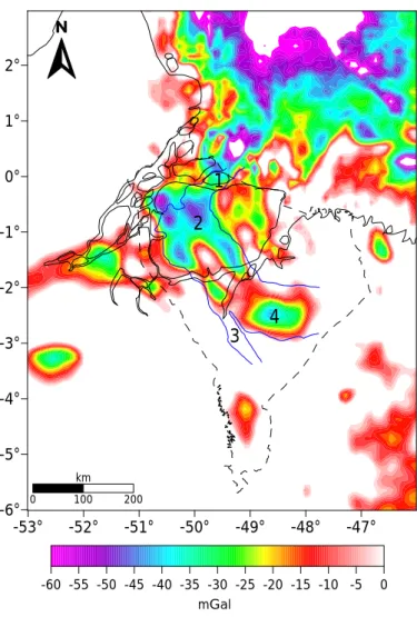
Figure 8 – Negative part of residual anomaly. Black dashed line represents the Marajó basin’s contour

while blue lines indicate the Marajó graben system. The numbers are (1) Mexiana, (2) Limoeiro, (3) Mocajuba and (4) Cametá sub-basins.

notable that the graben system is larger in NW direction, as well as the main part of residual anomaly. Figure 8 illustrates the negative-residual anomaly, which follows a NW tendency inside the Marajó basin.

Correlation with seismic interpretation

The seismic sections were, in essence, presented in an interesting study of Villegas (1994); Costa et al. (2002). They analyzed seismic reflection data with the purpose of mapping Marajó graben system, obtaining excellent results. From this point of view, we believe gravity and seismic data could provide a better interpretation when compared simultaneously. To do so, three

profiles in residual gravity anomaly were analyzed, due to the location of seismic data, aiming for plausible correspondence. Profiles A—B and C—D are located northward of Limoeiro sub-basin, while E—F profiles is near to Mocajuba and Cametá sub-basins. Figure 9a exhibits the location of each seismic section inside the residual signal and the seismic interpretation is presented in Figure 9b.

Profile A—B intersects the boundary of Marajó graben system west and eastward. This intersection is clearly visible in the seismic section. Negative high values in the profile of residual gravity anomaly could indicate the presence of normal faults in the east part. A second plausible indication of geologic faults would

-60 -50 -40 -30 -20 -10 0 mGal -53° -52° -51° -50° -49° -48° -47° -6° -5° -4° 0 100 200 km E F (a) (b)

Figure 9 – (a) Highlight of three gravity profiles on residual anomaly map. (b) Seismic sections inside Marajó graben system area, previously presented in Costa et al.

(2002).

be the tendency on residual signal, also sketched in seismic interpretation.

A second section C—D is located at east boundary of Marajó graben system. Similar to the A—B section, a negative high value is observed in residual anomaly. This low gravity zone can be associated to an existing sub-basin or geologic faults, once basin and faults normally show negative tendencies. Additionally, the uplift of igneous basement increases the value of gravity data, which is notable in the residual anomaly.

Profile E—F shows two significant faults and a possible formation of a horst-graben system, which in this case represent part of Marajó graben system. An interesting assumption is the depth of basement in seismic section, which decrease in SW-NE direction. Moreover, this tendency is clearly observed in the residual data, presenting a positive-negative trend.

CONCLUSIONS

Selecting the best gravity residual anomaly is a difficult task to perform when complex geological environments are present. With the purpose of improving regional-residual separation technique, we used a crustal modeling approach for separating regional and residual anomalies for gravity data. Our approach consists on

discretizing the Earth’s crust in rectangular prisms. Geometric parameters are defined by user, while top and bottom are set by topography and Moho surface. Therefore, residual anomaly is obtained from subtracting observed and predicted data.

We applied the former procedure at Marajó basin. The main reason lies on the lack of geophysical studies. Moreover, the presence of a known graben system intrigued us to go forward on interpreting this area. Despite geologically complex, crustal modeling approach clearly illustrated the Marajó graben system, mapped in former studies. To support gravity interpretation, a comparison with seismic data was done. Then, Marajó graben system observed from gravity data corresponds well when compared to seismic data. Geologic faults in the seismic section are seen as negative values in the gravity anomaly, while the rise of basement appears as a positive value and high tendency in the residual.

We believe the crustal modeling procedure was very interesting on selecting the best residual anomaly, providing a quite good interpretation despite the complexity of Marajó basin. At those types of geological environments, common techniques of separating regional and residual data are not recommended. Therefore, we also believe the presented approach is easily

applicable and quite appropriated for any Brazilian sedimentary basin, once all data set used in this work are free.

ACKNOWLEDGEMENTS

The authors would like to thank to Faculdade de Geofísica (portuguese version of Faculty of Geophysics) and Centro de Pós-Graduação em Geofísica (portuguese version of Geophysical Post-Graduate Center) for providing computational and financial supports. Third author has a special thank to Programa de Pós-Graduação em Geofísica, Observatório Nacional (ON/MCTI). The authors also appreciate the efforts of Dr. Boris Chaves Freimann, for help on geologic details and maps. Finally, the authors would like to thank the reviewers, for the significant assessments and suggestions in order to make this research better as well.

REFERENCES

AGOCS W. 1951. Least squares residual anomaly determination. Geophysics, 16(4): 686–696.

AL-HEETY EMS, AL-MUFARJI MA & AL ESHO LH. 2017. Qualitative Interpretation of Gravity and Aeromagnetic Data in West of Tikrit City and Surroundings, Iraq. International Journal of Geosciences, 8(02): 151. AMANTE C & EAKINS B. 2009. ETOPO1 1 Arc-Minute Global Relief Model: procedures, data sources and analysis. National Environmental Satellite, Data, and Information Service, National Geophysical Data Center Marine Geology and Geophysics Division, 19 pp.

AVENIUS CG. 1988. Cronostratigraphic study of the post-rift/sin-rift unconformity, Marajó Rift system. Belém, Brazil: Texaco/Canada Report. AZEVEDO RP. 1991. Tectonic evolution of Brazilian equatorial continental margin basins. Ph.D. thesis. Imperial College, University of London. 494 pp.

BELTRÃO JF. 1989. Uma nova abordagem para interpretação de anomalias gravimétricas regionais e residuais aplicada ao estudo da organização crustal: exemplo da Região Norte do Piauí e Noroeste do Ceará. Ph.D. thesis. Centro de Geociências, Universidade Federal do Pará, Belém, PA-Brazil. 156 pp.

BELTRÃO JF, SILVA JBC & COSTA JC. 1991. Robust polynomial fitting method for regional gravity estimation. Geophysics, 56(1): 80–89. BLAKELY RJ. 1996. Potential theory in gravity and magnetic applications. Cambridge University Press. 461 pp.

CARVAJAL DA, DORMAN JT, KENCK AR, KEY CF, MILLER CJ & SPECHT TD. 1989. Final report of the third exploration phase, Marajó. Belém, Brazil: Texaco/Canada. Report.

COSTA J, HASUI Y, BEMERGUY RL, SOARES-JÚNIOR AV & VILLEGAS J. 2002. Tectonics and paleogeography of the Marajó Basin, northern Brazil. Anais da Academia Brasileira de Ciências, 74(3): 519–531. FEDI M & QUARTA T. 1998. Wavelet analysis for the regional-residual and local separation of potential field anomalies. Geophysical Prospecting, 46(5): 507–525.

HACKNEY R & FEATHERSTONE W. 2003. Geodetic versus geophysical perspectives of the ’gravity anomaly’. Geophysical Journal International, 154(1): 35–43.

HINZE WJ, VON FRESE RR & SAAD AH. 2013. Gravity and magnetic exploration: Principles, practices, and applications. Cambridge University Press. 525 pp.

LI X & GÖTZE HJ. 2001. Ellipsoid, geoid, gravity, geodesy, and geophysics. Geophysics, 66(6): 1660–1668.

LUIZ JG & SILVA LMC. 1995. Geofísica de prospecção. Editora Universitária UFPA. Brazil. 335 pp.

NAGY D. 1966. The gravitational attraction of a right rectangular prism. Geophysics, 31(2): 362–371.

PLOUFF D. 1976. Gravity and magnetic fields of polygonal prisms and application to magnetic terrain corrections. Geophysics, 41(4): 727–741. ROBINSON ES. 1988. Basic exploration geophysics. Somerset, NJ (US); John Wiley and Sons, Inc. 576 pp.

ROSSETTI DF. 2010. Tectonic control on the stratigraphic framework of Late Pleistocene and Holocene deposits in Marajó Island, State of Pará, eastern Amazonia. Anais da Academia Brasileira de Ciências, 82(2): 439–449.

SCHALLER H, VASCONCELOS D & CASTRO J. 1971. Estratigrafia preliminar da bacia sedimentar da Foz do Amazonas. In: XXV Congresso Brasileiro de Geologia da SBG. São Paulo - SP, Brazil. Volume 3, p. 180–202.

SIMPSON JR SM. 1954. Least squares polynomial fitting to gravitational data and density plotting by digital computers. Geophysics, 19(2): 255–269.

SOARES JÚNIOR AV, COSTA JBS & HASUI Y. 2008. Evolução da margem Atlântica Equatorial do Brasil: Três fases distensivas. Geociências (São Paulo), 27(4): 427–437.

SOARES JÚNIOR AV, HASUI Y, COSTA JBS & MACHADO FB. 2011. Evolução do rifteamento e paleogeografia da margem Atlântica Equatorial do Brasil: Triássico ao Holoceno. Geociências, 30(4): 669–692. SPECTOR A & GRANT F. 1970. Statistical models for interpreting aeromagnetic data. Geophysics, 35(2): 293–302.

SYBERG F. 1972. A Fourier method for the regional-residual problem of potential fields. Geophysical Prospecting, 20(1): 47–75.