Instituto Politécnico de Tomar – Universidade de Trás-os-Montes e Alto Douro (Departamento de Geologia da UTAD – Departamento de Território, Arqueologia e Património do IPT)
Master Erasmus Mundus em QUATERNARIO E PRÉ-HISTÓRIA
Dissertação final:
A Quantitative analysis of European
Horses from Pleistocene to Holocene
NEELANSHU KAUSHIK
Orientadores: CARLOS LORENZO AND PROF. BENEDETTO SALA
Júri:
Ano académico 2008/2009
i
Abstract
Although so many articles have been published about the anatomy and systematic of Quaternary horse but still the story of Equus showing some missing links between the natural history of horse. In this present work applicant make an attempt to classify Horses (discriminate between species or group of species) on the basis of Size, Sex and shape analysis with using two Multivariate statistical methods. The objectives is two trace out the sex ratio, and establish degree of sexual dimorphism in fossil horses from Italian peninsula; to characterized the structure of horse bones on the basis of size and shape analysis occurs from Pleistocene to Holocene with the help of Mixture analysis and Principal Component Analysis. In the conclusion, one can say that the sex ratio is lying between 68%-32% approximately and also there is almost clear separation between the fossil data have been (they are not overlapping each other except Eisenmann Data which is a heterogeneous one) used in the present work in Size and Shape analysis, which indicating three factors that may be they have different taxonomy, different chronology and different environmental conditions. This present work is just a primarily attempt in Equine studies.
Key words: Quaternary Horses, Sexual dimorphism, Mixture analysis, Size analysis, Shape
analysis.
Resumo:
Embora se conheçam muitos artigos publicados sobre a anatomia e sistemática do cavalo do Quaternário, a história de alguns Equus mostra a falta de alguns elos de ligação na história natural do cavalo. No presente trabalho pretende‐se fazer uma tentativa de classificar Cavalos (discriminar entre espécies ou grupo de espécies), com base no tamanho, sexo e forma, com em dois métodos estatísticos. Os objectivos são traçar o racio sexual e estabelecer o grau de dimorfismo sexual nos fósseis de cavalos da península italian; caracterizar a estrutura dos ossos do cavalo, com base no tamanho e forma do Pleistoceno ao Holoceno, com a ajuda da análise e Mistura Principal de componentes de analises. Em conclusão, podemos dizer que a razão sexual está situada entre 68% ‐32% aproximadamente, e também que quase não existe uma separação clara entre os dados dos fósseis, (não são sobrepostos uns aos outros, excepto os Dados de Eisenmann, que são heterogénios) utilizados no presente trabalho, na análise do tamanho e formato, o que indica três factores que podem ser os que têm diferentes taxonomía e cronología e diferentes condições ambientais. O presente trabalho é apenas uma tentativa de estudo dos Equinos.Acknowledgement
From the very first time at Macao in Portugal, Prof. Luiz Oosterbeek, softly but surely drilled about the European Archaeology as a part of adventurous trip to cadaval cave. He taught me about the relevance of archaeology, central to our very roots as Homo sapiens sapiens. It has helped me in my pursuits of understanding the “Holistic Past” that has a potential of becoming ‘a key to the present’. For all time, he encouraged me to go through the diversity of Archaeology; he supported me in all the circumstances. I will highly grateful to him for his all support and for becoming optimistic about my interest in Quantitative Analysis.
Then, followed, my curiosity to understand the Role of Quantitative Analysis in Archaeology that have contributed to preserve the records from the sites and try to give relevant solution of the problem. Hence, for my thesis when I approached the director of my thesis Carlos Lorenzo Merino, paleoanthropologist in URV, Tarragona in Spain, expressing my desire to learn some applications of statistics in Archaeology, he agreed and always encourages me for doing my best. Carlos’s friendly personality as well as his interest and knowledge encourage me to reach the result of my thesis without their unflinching support and guidance this dissertation would not have materialized. I have immensely benefited from his guidance that has been an experience to live with.
Overall, the supervision of my research guide Dr. Benedetto Sala, Paleontologist and his experienced suggestions have greatly helped me in shaping the present work. Both of my Supervisors have been the most inspiring Professor whose invaluable guidance in the present work is phenomenal. I would like to thank Prof. Rober Sala to permit to attend the classes in URV, Tarragona, which really helped to make a vision about my thesis.
As a novice, while learning to stand on my own feet in the world of Prehistory and Quaternary, I received untiring and inspiring help from some of best researchers, viz. Dr.
Sara cura, Dr. Mila, Dr. Rosina, Dr. João Baptista, Dr. Marta Murano, Dr. José Mateus, Dr. Paula Queiroz, Dr. Simon Davis, Dr. Marta Azzerello, Dr. Ursula and Dr. Marsha Levine. These entire scholars did not hesitate, even in sending their publications, giving invaluable suggestions and a big part of encouragement for which I am extremely indebted and grateful.
I am immensely thankful to the European Commission for providing me the Erasmus Mundus Fellowship for pursuing this European Master in Quaternary and Prehistory.
My sincere thanks go to Marco Rustoni, Italy (Florence) for guiding me about taking the measurement of Horse bones. He provided me all necessary help and important data of horse during my mobility to Italy.
Prof. Jan van der Made is also thanked immensely for his guidance, comments, advises and support. He is not only provided information about this course but also encouraged me in pursuing my interests.
I sincerely thank all the members of Macao Museum for their generous support and kind helps during the stay in Portugal and preparation of this master thesis. Sincere thanks to all the academic and non academic staff of University of Ferrara, Italy for their generous help and support during my mobility in Italy.
My heartfelt thanks go to Dr. Vijay Sathe, who has been my mentor in all these years and helped me develop a vision for the subject. He has been a source of constant encouragement and support. Without his support this dissertation would not have been possible.
I am immensely thankful to my Portuguese teacher Susana, because of her only I was able to spend my time in communication in Portugal. I would like to thank Catarina and other staff to keep informing me about each and every detail.
This dissertation would not have come through without the support and help of my friends throughout the journey of this master program, Flavio, Hugo, Peich, Cris, Ellian, Ana
Carolina, Tosa banta, Renata, Jayshree, Xiling day, Redha Benchernine, Souhila roubach, Saloua, Jorge, Fatimah, Luna, Ruman, Arun, Anjar, Madhavi, Hemu, Sarathi, Tesagi, Isabel, Kamal, Filip, Guliarmo, Judith, Neilson, Andera and Chowlawit are beyond words.
I would like to say warmly thanks to Neetu Agarwal, Sayantani Neogi, Nadia kandi, Hocine Belahrache, and Venkatesan Jambunathan; they always stand with me in every situation and provide me mental support to complete my work.
Without the support of Shikha this thesis would not have materialized. She has always been there to help me in all aspects. She patiently helped in preparing the bibliography and illustrations and proof-reading the draft.
Last but not the least I would like to express absolute gratitude to my parents and all my family for standing by and encouraging me through the entire course. Their emotional and moral support and love cannot be expressed in words.
List of Tables:
Table 1: classification of sites, chronology and fauna. Table 2. Variables used in Mixture analysis
Table 3. Results of mixture analysis of 1st Phalanx anterior of fossil horse. Table 4: Results of mixture analysis of 3rd phalanx anterior of fossil horse Table 5: Result of mixture analysis of Astragulus of fossil horse
Table 6: Result of mixture analysis of Calcaneus of fossil horse. Table 7: Result of mixture analysis of Humerus of fossil horse. Table 8: Result of mixture analysis of the Upper teeth of fossil horse
Table 9: Result of Mixture Analysis of the Geometric mean of given variables. Table 10: Eigenvalues and % of Variance and PC1 & PC2.
Table 11: Eigenvalues and % of Variance and PC1 & PC2. Table 12: Eigenvalues and % of Variance and PC1 & PC2.
Table 13: Eigenvalues and % of Variance and PC1, PC2, PC3 & PC4. Table 14: Eigenvalues and % of Variance and PC1 & PC2.
Table 15: Eigenvalues and % of Variance and PC1, PC2, PC3 & PC4 Table 16: Eigenvalues and % of Variance and PC1 & PC2
Table 17: Eigenvalues and % of Variance and PC1 & PC2 Table 18: Eigenvalues and % of Variance and PC1 and PC2.
Table 19: Eigenvalues and % of Variance and PC1, PC2, PC3 and PC4. Table 20: Eigenvalues and % of Variance and PC1.
Table 21: Eigenvalues and % of Variance andPC1, PC2 and PC3. Table 22: Eigenvalues and % of Variance and PC1 and PC2. Table 23: Eigenvalues and % of Variance and PC1 and PC2.
List of Figures:
Figure 1: Horse evolution: sketches of body form, front limb, skull and upper molar in occlusal and lateral views
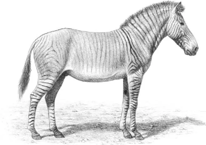
Figure 2: Reconstructed life appearance of the Equid
Figure 3a). Mixture Distribution of Maximum length of the 1st phalanx (from fossil sites) dimensions as a test
Figure 3b). Mixture Distribution of Minimal Breadth of the 1st phalanx (from fossil sites) dimensions as a test case.
Figure 4: Mixture Distribution of Maximum height of 3rd phalanx dimensions.
Figure 5: Mixture Distribution of Maximum height of Talus from the fossil sites dimensions.
Figure 6: a) Mixture Distribution of Maximum Length of Calcaneus from the fossil sites dimenisons.
Figure 6: b) Mixture Distribution of Maximum medial depth of Calcaneus dimensions. Figure 7: Mixture Distribution of Minimal Trochlear height of Humerous from the fossils sites dimensions.
Figure 8: a) Mixture Distribution of 2nd Premolar height of the upper teeth from the fossil horses.
Figure 8: b) Mixture Distribution of the Breadth of 3rd/ 4th Premolar of the Upper teeth from the fossil horses.
Figure 9: Principal component analysis of Astragulus a) showing variability in size; b) showing variability in shape.
Figure 10: Principal component analysis of Calcanium a) showing variability in size; b) showing variability in shape.
Figure 11: Principal component analysis of Humerus a) showing variability in size; b) showing variability in shape.
Figure 12: Principal component analysis of Meta carpal a) showing variability in size; b) showing variability in shape.
Figure 13: Principal component analysis of Meta Tarsal a) showing variability in size; b) showing variability in shape.
Figure 14: Principal component analysis of Tibia a) showing variability in size; b)showing variability in shape.
Figure 15: Principal component analysis of Tibia a) showing variability in size; b)showing variability in shape.
Figure 16: Indication of Positive axis and Negative axis in PC1 and PC2.
Index
Abstract(English)………. ….i Abstract (Portugues)………. ii Acknowledgement………iii-v List of Tables………vi List of Figures………...vii-viii Chapter 1 Introduction 1-5 Chapter 2Natural History of Horse 6-18 Chapter 3 Quantitative analysis of Horse bones 19-56 Chapter 4 Discussion and Conclusion 57-62BIBLIOGRAPHY 63-72
1
CHAPTER 1
Introduction
The word ‘horse’ originally meant the domestic horse. It is still used mainly in that sense, just because these are the horses, we usually talk about in ordinary conversation, but then there are wild horses, too. How can we differentiate that they are a sort of horses, and yet not the same as the domestic horse? Then there are donkeys, zebras, onagers, but not the same as domestic or wild horses. We need some way to indicate that they are horses of a sort and yet that they are not domestic horses and differ more from domestic horses than wild horses do.
Although a number of recent publications deals with the anatomy and systematic of Quaternary equids, (e.g. Azzaroli 1979, Bennett 1980, Eisenmann 1980,1981, Groves/ Willoughby 1981) the Story of Equids is still alluring and exasperating after 150 years, during which time it has attracted researchers and fed their debates. The fossil material is rich enough to raise hopes, but not rich adequate to fulfill them. The variety and profusion of data exercises such constraints on interpretations that they rarely remain simple and conclusive (Eisenmann et al 2002).
But one thing is clear that further work is needed to perquisite are knowledge of their topical history and to answer such questions as: What species of Equus was (or were) domesticated? When? Where? Apparently, no progress in the considerate of the geographical and chronological distributions of domesticated and wild forms can be expected if one is not able to discriminate the osteological remains of the different species and varieties of Equus.
2 Simply one can say that there is some problem to discriminate the horses (discriminate between species or group of species) on the basis of Size and shape, whether it is a wild form or domestic form? Which Equus sp. it is? The same problem is related with sex ratio as sex ratios in fossil animals can provide important information regarding the biology and behavior of animal populations as well as the agents responsible for the collection of fossil bone assemblages (Klein & Cruz-Uribe, 1984: 90–92; Davis, 1987: 44–45). In the site, most of the time it is difficult to discriminate the sex, whether is it a male or female? Reminding all the things, Applicant is trying to make an attempt to do the discrimination in sex, size and shape with the use of Quantitative analysis in this thesis.
Popular interest in horses arises mainly from the fact that they are the animals admired by everyone regardless whether or not we had any acquaintance. It so, how and when it all began to tame this animal and/or what were the causative factors behind such a phenomenon, and how has it evolved from its primitive ancestors, underlines the very objective of this piece of research.
Objectives:
1.
To determine the sex ratio between the given populations of Italian Sites of fossil horses.2.
To find out the degree of Sexual dimorphism per skeletal part.3
4.
To define the structures of horse bones on the basis of changes occurs in shape of horse bones from Pleistocene to Holocene.Methodology:
There are two kind of data used in this analysis, one is Fossil one which belongs to Italian peninsula and the chronology is middle Pleistocene and Upper Pleistocene, and other one is Modern horses and the applicant has derived the information regarding modern horses as well as the published data from Vera Eisenmann, who is one of the pioneer scholar in equine studies. The Methodology is based on two statistical methods one is Multivariate i.e. Principal Component Analysis and another is Mixture analysis. Principal Component is applied to trace the changes in horse bones on the basis of Size and Shape, While Mixture analysis is applied to define the sex ratio as well as find out the degree of Sexual Dimorphism in the Fossil horse bones.
Chapterization:
Chapter 1 deals with the introduction to the basic idea of this research and discusses very briefly the Objectives and Methodology of this study. It also provides a brief review of Quantitative methods in Archaeology.
Chapter 2 begins with a natural history of horse, where records available in the slices of time in geology. However, when one attempts to make a meaningful survey of such a record, he is often confronted with data scattered in several fore irrespective of its geographical distribution. Hence the question comes up as to who where its ancestors? How and where did it evolve, and how old is the Natural History of this animal in
4 Europe? The applicant has putted all the things together, while they are highly debated, showing controversies there applicant trying to indicating the way to find the solution may be towards Quantitative Analysis.
Chapter 3 constitutes the main body of this thesis. Here applicant explains Materials and Methods used in analysis, Applicant also provide the brief role of Statistical Methods used in this chapter. It shows the results of Mixture Analysis, Size and Shape Analysis. Chapter 4 is a summary of the research results and conclusions with a discussion of how the research goals were addressed. Additionally, directions for future research have been suggested.
A Brief History of quantitative methods
The quantitative analysis has a quite long history, the scope of this disciple broadened in the early 19th century to include the collection and analysis of data in general. In the same period applications of quantitative methods in biology had been started, and this separate branch is called Biometry. The early work of the biometric laboratory established by Galton and Pearson bears witness to the vital interplay between the development of statistical methodology and anthropological research (e.g., Mahalanobis, 1928, 1930; Morant, 1928, 1939; Pearson, 1903, 1933). In 1917 D’Arcy Wentworth Thompson published his remarkable treatise on growth and form (Thompson 1917). This volume is replete with captivating suggestions, indicative of deep insight into the fundamental concepts in the study of change in shape. Beginning with some exploratory work by Teissier (1938), the algebraic mode of analysis in the form of principal components surged to the fore. Teissier’s results involved what we would now call Allometric size
5 change. In this new age so many scholars published their works, which were first applications towards this revolutionary time and related to the role of quatitative methods and computers in Archaeology. Like Bohlers (1956): Graphics & Statistics; Heinzelin (1960): Statistics. Sokal &Sneath (1963): Numerical taxonomy; Kruskal (1971): Seriation by multidimensional Scaling; Benzecri (1973): Correspondence analysis; Doran & Hodson (1975): Mathematics & Computers in Archaeology; Djindjian (1976): Correspondence analysis in Archaeology; Hodder & Orton (1976): Spatial Analysis in Archaeology and Tukey (1977): Exploratory data analysis.
Hopwood (1936) proposed a couple qualitative features to discriminate horse from ass and zebra and vice versa. Skinner, Macfadden and Vera Eisenmann gave remarkable approaches about Biometry and morphometry. The number of Paleontologists has given a set of cranial, dental and skeletal parameters that have enabled a definite equine identification (Skinner 1972; MacFadden 1992; Eisenmann 1986).
CHAPTER 2
Natural History of horse
Horse appears in very oldest graphic records made by man; Stone Age paintings made long before writing was invented. Between these dates, a roster of writers who have discussed horses would include most of the stalwarts of literature and natural history. Homer to Aristotle; Shakespeare and from naturalists are Cuveir, Agaziz, Cervantes to Darwin; to name a few, who have devoted much of their attention to the art and science of horses and it will continue to be a subject of study for many more people in years to come in future. Here in this chapter applicant try to squeeze the natural history of horse at the same time as the taxonomic position of equine is highly debated among different authors.
Taxonomy of Equus
Genera and Subgenera of the Equidae
Equus is a genus of the animals exists in family Equidae and it is in central to the concept of horse systematic. As Morris Skinner (1972) so aptly noted, this genus also is exemplary of the problems confronting palaeontologists in synthesising consensus phylogenetic schemes for taxa that contain fossil and extant representatives using different sets of characters. To compound the problems surrounding this already complex genus, the taxonomic literature on Equus contains about 230 named species (Winans, 1989), many of which are based on very fragmentary material or have inadequate description. Of these, 58 have been allocated for North American fossil species, which Winans (1985, 1989) synonymizes into five valid taxa. The first who presented a classification of equine was Lydekker (1907), who split the genus into four subgenera: Equus including horses and hemionus; Hippotigris including Mountain Zebra and Burchelli; Dolichohippus including
zebra and Asinus, wild donkeys. In the Following many authors among which shortridge (1934), stehlini and Graziosi (1935), Ellermann and Morrison-Scott (1951), Ellermann et
al (1952), Quinn (1955), Trumler (1961), Azzaroli (1966), Groves and Mazak (1967),
Bennet (1980), Groves (1986) and Azzaroli and Stanyon (1991) have addressed the systematic equine considering dental characters and the characters of the cranial and postcranial.
Antonius (1912) recognized nine “recent and quaternary” species of wild horses in Europe. Some of these (E. suesenbornensis, E. mosbachensis) are middle Pleistocene; some (E.
woldrichi, E. abeli) are of uncertain age; and two (E. gracilis, E. sequianus) are based on
hypotheses and not on specimens as such, although a skull was assigned to the latter on a provisional basis. Antonius (1912) was quite clear that domestic horses have a multiple origin, and Equus gracilis of Ewart was recognized in clear expectation that this reconstructed gorse would be found as a fossil as had Equus sequianus of Sanson.
Samson (1975) has recently proposed an extremely elaborate scheme in which horses are even divided into three subgenera (Equus, Microhippus, and Euhippus). It is difficult to know exactly what to make of his scheme since it is based entirely on dental characters and must be tested out on cranial characters before it can be confirmed.
A remarkable essay by Bennett (1980), attempts to refine such unwieldy schemes as the six-subgenus arrangement by the use of cladistic analysis. This method tries to find out which character states are primitive and which are more evolved. Characters in which two or more groups show derived states in common are then sought, and the greater their number the more plausibly the taxa are seen to be related. Eisenmann (1980) used totally different methods from Bennett (1980) and arrives at results that go some way towards bridging the gap between the other two studies. Her (Eisenmann, 1980) results lead her to emphasize the
strong differentiation between the six sub generic groups. At the end of her monograph she tries different ways of linking groups together and suggests that the most parsimonious one, with many caveats, might be one which is, in effect rather similar to that of Bennett (1980), although the most plausible, tie between two groups would be between asses and hemiones.
Groves/Willoughby (1981) reviewed the available evidence and decided that as a conservative measure, six subgenera ought to be recognized. First one was Asinus , which has a short scapula, relatively long skull, very short and narrow distal phalanges on each extremity, short palate, long diastema (longer than premolar row), pterygopalatine fossa visible in ventral view, upturned occiput, and many other distinguishing characters.
Hemionus has, in some respects, a similarly proportioned postcranial skeleton but also has
very long slender metapodials and a longer distal phalanx, a very narrow occipital crest, shortened postorbital part of the skull, long vomer, short diastema, pterygopalatine fossa concealed by backward extension of malar tuberosity, upturned occiput, and so on. Equus has a long scapula, smaller skull relative to postcranial elements, stout metapodials and phalnges, long rounded occipital crest, long diastema, and fossa visible. The three subgenera (Hippotigris, Quagga, Dolichohippus) containing striped species, Zebras, differ in other respects, but Zebras are marginal to the area under discussion unless Equus hydruntinus is really a Zebra (Groves/Willoughby 1981).
There are three categories of the enamel pattern of the lower cheek teeth of grazing equids: the "hipparionid", the "caballoid", and the "stenonid" pattern, mainly defined on the configuration of the metaconid and metastyld of the double knot (Groves (1986). Groves (1986) has proposed E. ferus to replace E. caballus, because Linnaeus' type was a domestic horse; Azzaroli (1995), Eisenmann and Turlot (1978), Groves (1986), Groves and Willoughby (1981), Heptner et al. (1961), Kurtén and Anderson (1980), and Skorkowski (1938) provide taxonomies and reviews of species. There is another theory which is based on
replacement of stenonoid by caballoid horses in Europe by Forsten (1998) which occurred in the Villafranchian, although she earlier (Forsten, 1986) agreed with the general view that this replacement occurred in the Galerian.
Bennett followed Trumler (1961) and recognised seven living or recently extinct subspecies, which are listed below (Bennett, 1992b). Their characters inferred, from the morphology and distribution of late Pleistocene to early Holocene fossils, historical descriptions of Eurasian wild horses, and finally, the characters of the early breeds of domesticated horses. Genetic analysis based on chromosome differences (Benirschke et al., 1965) and mitochondrial genes both indicate significant genetic divergence among the several forms of wild E. caballus as early as 200,000 – 300,000 years ago, long before domestication (Azzaroli, 1990). Thus, these diverging ecomorphotypes were, in various parts of Europe, domesticated in parallel; for example, the tarpan (E. c. ferus) in the steppe region of Eastern Europe, and the warmblood (E. c. mosbachensis) in central Europe (Azzaroli, 1990).
E. c. alaskae Hay, 1913:2, 3. Lamut, or Beringian Horse.
E. c. caballus Linnaeus, 1758: 73. Northwestern European Horse.
E. c. ferus Boddaert, 1785: 159. Tarpan (gmelini Antonius, sylvestris Brinken are synonyms.
E. c. mexicanus Hibbard, 1955. American periglacial Horse.
E. c. mosbachensis von Reichenau, 1903: 583. Central European Horse.
E. c. przewalskii Polyakov, 1881: 1. Przewalskii Horse, Mongolian Wild Horse.
Diagnosis
Family Equidae Gray 1821:
Completely molarized upper and lower P2-M3; tridactyl manus and pes (MacFadden 1986); metacarpal 5 reduced; I1-3 with pitted crowns, extented premaxilla, lower diastema; angle of jaw posteriorly rounded, without notch (Prothero & Schoch 1989). “Anchitheriinae” sensu
strict is greatly increased tooth crown area and estimated body size (MacFadden 1984, 1986);
loss of ribs between styles on cheek teeth (Stirton 1940; Forsten 1986).
Subfamily Equinae Gray 1821:
Cement formed on deciduous and permanent cheek teeth; degree of development of pli caballin on premolars and molars; presence of pli entoflexid; moderately deep ectoflexid on P2; unworn m12 molar crown heights greater than about 23-28mm (Hulbert & MacFadden 1990).
Tribe Hipparionini Quinn 1955:
Diagnosis:
Hipparionini are typically small, narrow- bodied, light weight, agile and dainty, they have extremely hypsodont teeth with highly complex structure (Bennett, 1992). Well-developed and persistent pli caballin on molars; MC 5 articulates primarily with MC 4 (Hulbert & MacFadden 1990).
Tribe Equini Gray 1821:
Dorsal preorbital fossa (DPOF) depth moderate; DPOF with shallow posterior pocket; protocone-protoloph connection during early wear stages on P34; hypoconid lake on P34; p34 metastylid much smaller and located more lingually than metaconid; m12 metastylid much smaller and located more labially than metaconid; (Hulbert &MacFadden 1990).
Genus Equus Linnaeus 1758:
Diagnosis:
DPOF poorly developed or absent; very high crowned and relatively straight teeth; complex enamel plications and protocones (Bennett 1980; Azzaroli 1982; MacFadden 1984); elongated and either robust or gracile metapodials (Bennett 1980; Forsten 1986); well-developed intermediate tubercle (INT) on distal humerus (Hermanson & MacFadden 1992).
Equus caballus has, on average, the heaviest body build, the widest and deepest head, and the
heaviest limbs of any of the six to eight living and one recently extinct (E. quagga) species in the genus (Eisenmann, 1980). However, there is great variation in size and proportions among domesticates. The skull is elongated (>500 mm); orbits large and oriented dorsolaterally; molar row long (>80mm); and incisor region broad (Osborn, 1912). Upper cheek-teeth large, usually with long, bipartite protocones connected to the protoloph; hypoconal groove deep (Quinn, 1955). Edges of pre- and post-fossettes more intensely folded than in congeners (McGrew, 1944). The lower cheek teeth are characterized, as in other caballoid horses, by a U-shaped entoflexid between the metaconid and metastylid, in contrast to stenonids, which have a V-shaped entoflexid (Forstén, 1986). Hooves are roundish, shorter ear (<20cm), and tail much more fully haired than in Onegers (Willoughby, 1974).
Evolution of Horse
“The geological record of the Ancestry of the Horse is one of the classic examples of evolution” -- Matthew (1926; 139)
The genus Equus has had a widespread and complex bio-geographic history. The earliest fossil Equus found in the New World dates to about 3.7Ma (Lindsay et al. 1980). Some of the first perissodactyls were horses, no larger than a terrier admittedly, but the first in what has come to be regarded as an evolutionary classic (Simpson, 1961; MacFadden, 1992). Major changes may be observed during the history of the horses (Figure 1) reduction in the number of toes from four (front) and three (back) in the first horse Hyracotherium, to three in
Mesohippus and one in Pliohippus and, independently, in modern Equus; and a deepening of
the cheek teeth from small leaf-crushing molars to the deep-rooted grass-grinders of modern horses (Savage and Long, 1986). The changes in limb structure and teeth are linked to the overall increase in body size that occurred during horse evolution (Savage and Long, 1986).
These changes described by a major environmental change that has been taken during the late Oligocene and early Miocene: the spread of grasslands in North America. Early horses, such as Hyracotherium, Mesohippus and Parahippus, were browsers that fed on leaves from bushes and low trees (Froehlich, 2002). As the forests retreated and grasslands spread, new horse lineages, such as Merychippus and Hipparion, stepped out on to the plains and put their reinforced molars to work (Savage and Long, 1986).
Applicant described the evolutionary story in two events. The First main event was the arrival of Hipparion, they arose in North America during the middle Miocene and differed significantly from Anchitherium and other early and middle Miocene equids in a number of respects (Bernor and Armour-Chelu, 1999). While the low crowned, three-toed horses of the
genus Anchitherium succeeded in the Laurophyllous forests of Europe, in North America the extension of more open woodlands in the middle Miocene led to the appearance of new kinds of equids, characterized by their hypsodont dentition and slenderer limbs (Garces et al 1997). This group, derived from Merychippus, developed highcrowned cheek-teeth as a response to the more sclerophyllous, harder vegetation and Moreover, the tooth enamel became folded in several ridges, which, in turn, filled with dental cement (Garces et al 1997). With little variation, this kind of molar characterizes all modern horses, today’s representatives of Equus included (Garces et al 1997). Simply equids appear especially well suited to survive in poor habitats, where only low-energy food such as grass is available (Janis, 1976).
The second main event, shortly after the entry of the first Mammuthus, was the replacement of the last Hipparion by the first true horses of the genus Equus (Franzen, 1995). As at the beginning of the late Miocene, when Hipparion replaced the last Anchitherium, the history of an American equid replacing the old autochthonous form was repeated (Bernor and
Armour-Chelu, 1999). The first Equus originated in North America from advanced equids like
Pliohippus, which increased their size and hypsodonty and reduced the number of toes from
three to one.
At about 2.6 million years ago (almost coinciding with the boundary between the geomagnetic epochs Gauss and Matuyama), these first representatives of the genus Equus dispersed into Eurasia, the oldest ones having been found in Siwaliks, Pakistan, and the Cabriel Basin, Spain (Garce´s et al 1997).
Figure 1: Horse evolution: sketches of body form, front limb, skull and upper molar in occlusal and lateral views. The whole-body restorations, skulls and teeth are drawn to scale, and the legs are drawn to a standard length. Note the major changes in the skull and teeth when dietary habits changed from browsing to grazing. (Based on Savage and Long, 1986)
The last hipparionine equids of this time belonged to the species Hipparion rocinantis, known from a number of sites in southern Europe (Villarroya, Spain; Perrier-Roccaneyra, France; Kvabebi, Georgia), Curiously, H. rocinantis was a large, and highly hypsodont and robust form, similar in many respects to the first true horses of the genus Equus (Garces et al
1997). This was probably a result of the parallel adaptation to the development of grasslands and prairies over extensive areas of Europe and North America.
Among the first European Equus was Equus stenonis, which has been found in several localities of western and eastern Europe and included several subspecies (E. s. stenonis, E. s.
livenzovensis, E. s. vireti, E. s. senezensis, and others) (Figure 2) (Agusti and Anton, 2002). In general, they were large, quite robust horses between 1.3 and 1.5 m at the withers. Some slender relatives of E. s. stenonis (E. s. granatensis and E. altidens) lie probably close to the origin of the hemions and asses (E. hydruntinus), while the origin of African zebras appears to be close to some evolved forms of this species (Agusti and Anton, 2002).
The stenonian horses, derived from Equus stenonis, also diversified at the end of the early Pleistocene into a number of species. Some of them were large, such as E. sussenbornensis, which stood about 1.8 m at the withers and showed characteristics leading in the direction of the modern horse (E. caballus) (Garce´s et al 1997). Others, on the contrary, were small and slender, such as E. stehlini and E. altidens, the latter probably related to today’s hemiones (Garce´s et al 1997).
Equus stenonis although the stenonine horses belonged in the same genus as all of today’s equids, their appearance would have been different because of their large, elongated skulls. This restoration, based mostly on material from the site of Saint-Vallier, shows the long muzzle and concave dorsal profile typical of Equus stenonis. (Agusti and Anton, 2002).
Figure 2: Reconstructed life appearance of the Equid (Source: Agusti and Anton, 2002).
In the case of Equus, the first modern horses related to the present day E. caballus appeared at this time (E. germanicus and E. mosbachensis) and replaced most of the more slender stenonian species (MacFadden, 1992). These middle Pleistocene horses were, in general, larger and more robust than the species of the early Pleistocene and better suited for the cold, steppe landscapes of the middle Pleistocene (MacFadden, 1992). Some small stenonian horses persisted into the middle Pleistocene (E. altidens) and probably even reached the late Pleistocene (E. hydruntinus) (Garces et al 1997). E. caballus and E. hydruntinus are also often found together, and in frequently large herds, especially in the course of the Last Glaciation (Caloi, 1997). It would therefore seem that the very extreme climatically situations allowed the survival of several taxa. One possible explanation of this phenomenon could be in the greater fragmentation and diversification of the habitats, which accompanied the glacial periods, especially in the second part of the Pleistocene, which also sees the shifting
both in altitude and latitude of the vegetational belts (Gingerich, 1984; Graham & Lundelius, 1984).
During the Upper Pleistocene, there is good evidence for one additional species within the Plains zebra group, E. capensis from South Africa (Thackeray, 1992); at least two more within the Asinines, E. melkiensis (Bagtache et al., 1984) from North Africa and E.
lauracensis (Astre, 1948) from France; another Hemionine, E. hydruntinus (Burke et al
2003); and at least two of unknown affinities. E. graziosii at Maspino from Italy (Azzaroli 1966) and E. valeriani from Uzbekistan (Eisenmann et al., 2002).
Caballines include at least three morphologies: the ubiquitous heavy horse (known by such names as gallicus, germanicus, latipes, uralensis, lenensis, lambei) the giant horse of San Sidero, Italy and the southern light horse, E. antunesi, of Italy and Portugal (Cardoso and Eisenmann 1989). There is also a Caballine, E. algericus, from North Africa (Bagtache et al., 1984).
The story of the horses has become a textbook example of ‘progressive evolution’ or a ‘trend’ as there seems to be a clear-cut one-way line of change from the small leaf-eating
Hyracotherium to the large grazing Equus.
Prehistoric Association:
The oldest known record of this association which may have been a mere acquaintance with horse, comes from middle Paleolithic cave paintings in France and Spain that probably are between 35,000 and 100,000 years old. In the new world, horses are believed to have become extinct at the end of the Pleistocene; as a part of ‘great mega-faunal extinction’ about 11,000 years ago (Meltzer and Grayson, 2003). Although, Clutton-Brock (1981) believes that they may have persisted into historical times. Therefore, the horses that were so abundant during
the late Pleistocene were conspicuously absent from the later faunas. Horses were reintroduced into the New World by Spanish explorers during the 16th century.
In the Old World, however, wild equids including horses and their relatives (zebras, onagers and asses) persisted into the Holocene. So far as is known, horses were domesticated during the late Neolithic, probably by the end of 4th or the beginning of the 3rd millennium B.C. Though not accepted universally, domesticated horses probably descended from tarpan (which became extinct in the wild in 1851) (Zeuner, 1963), in Western Europe or from
“Przewalski’s horse” in the high arid steppe regions of eastern Asia; where it is still living. It
is also believed that the other species of the genus Equus, including wild assess and their relatives were originally domesticated in Africa and possibly southern Asia.
Althought a number of recent publications deals with the anatomy and systematic of Quaternary equids, but it is clear that much more work is needed to perk up are knowledge of their topical history and to answer such questions as: What species of Equus was (or were) domesticated? When? Where? Apparently, no progress in the understanding of the geographical and chronological distributions of domesticated and wild forms can be expected if one is not able to discriminate the osteological remains of the different species and varieties of Equus. Briefly, all the same, further research will be necessary in order to have a better knowledge of the relationship between morphology and environment. In the same process, applicant is trying to make an attempt to see the relationship between Equus caballus And
CHAPTER 3
Quantitative analysis of Horse bones
1. Materials and Methods:
1.1. Materials
There are two kind of data used of horse bones in this chapter, one is Fossil forms and another one is Modern forms. Fossil horse data came from eight different sites from Italian peninsula. Some of these sites fit in to middle Pleistocene and some belong to Upper Pleistocene. Sites are following:
Sites Chronology Fauna
Cardamone Upper Pleistocene Equus caballus Melpignano Middle/Upper Pleistocene Equus caballus.
Maspino Upper pleistocene Equus graziosii
Valdichiana Upper Pleistocene Equus caballus Castel di Guido Middle Pleistocene Equus caballus
Paglicci Middle/ Upper Pleistocene Equus caballus, E. hydruntinus
Romanelli Upper Pleistocene Equus hydruntinus, Equus sp. Polesini Upper Pleistocene Equus caballus, E. hydruntinus Table 1: classification of sites, chronology and fauna.
Modern horse’s data came from Vera Eisenmann’s website. In this modern data Equus
caballus and E. c. przewalskii is present. Eisenmann data is heterogeneous.
20
Applicant used Eisenmann Parameters for measuring the bone and the Skeletal Part which used in this process is Humerus, Radius, tibia, Upper Teeth, Metapodials, Astragalus, Calcaneus, 1st phalanx and 3rd phalanx. Applicant used bones according to the accessibility of data. In ‘Mixture analysis’, the used bones are Humerus, Talus, Calcaneus, 1st phalanx, 3rd Phalanx and Upper teeth. Variable definitions are given in Table 2.And for another statistical method ‘Principal Component Analysis’ used bones are Talus, Calcaneus, Humerus, Femur, Radius, Tibia, Mandible, Metapodials and Upper teeth.For making this entire analysis researcher used PAST software (Paleontological Software).
Table 2. Variables used in Mixture analysis
1st Phalanx: Maximum Length Minimal Breadth, Proximal Breadth, Proximal Depth, Distal
Breadth of tuberosities (DBT), Distal Articular Depth (DAD).
3rd Phalanx: Length from the Posterior Edge of the Articular surface to the tip of the
Phalanx, Anterior Length, Articular depth, Maximum Height, Angle Between the sole and the dorsal line, Circumference of the sole.
Calcaneus: Maximum Length, Length of Proximal Part (Length prox), Minimal Breadth,
Proximal Maximal breadth (PMB), Proximal Maximal Depth(PMD) , Distal Maximal Breadth (DMB), Distal Maximal depth (DMD).
Humerus: Maximal length, Maximal length from caput (MLC), Minimal Breadth, Diameter
perpendicular to and at the level of 3, Proximal maximal breadth (PMB), Proximal depth at the level of the median tubercule (PDMT), Maximal Breadth of the Trochlea (MBT), Diastal maximal depth (DMD), Maximal Trochlear height medial (MTH), Minimal Trochlear height in the middle (MiniTH), Trochlear height at the sagittal crest (TH).
Upper teeth: Length, Breadth and Height of P2 (P2L, P2B, P2H), Length, Breadth and
Height of P3/P4 (P3/P4L, P3/P4B, P3/P4H), Length, Breadth and Height of M1/M2 (M1/M2L, M1/M2B, M1/M2H), Length, Breadth and Height of M3 (M3L, M3B, M3H).
Metacarpal: Maximal Length, Medial Length, Minimal Breadth, Depth of the diaphysis at
the level of 3, Proximal articular breadth (PAB), Proximal articular depth (PAD), Maximum Depth of Articuler Facet(MDAF), Diameter of Anterior Facet of Fourth Metacarple( DAFF), Diameter of the Anterior Facet of Second Metacarpal(DAFS), Distal Maximal Supra Articuler Breadth( DMSAB), Distal Maximal Articuler Breadth(DMAB), Distal Maximal Depth(DMD), Distal Minimal Depth of Lateral Condyle(DMDLC).
Mandible: Length, Muzzle length, Premolar length, Height of the Ascending Ramus (HAR),
height of the jaw posterior to M3 (HJP3), height of the jaw between P4 and M1 (HJP4M1), Height of the Jaw in front of P2 (HJP2).
Metatarsal: Maximum Length, Medial Length, Minimal Breadth, Depth of diaphysis at level
3, Proximal Articular Breadth(PAB), Proximal Aticular Depth (PAD), Maximal Diameter of Articular Facet for the third Metatarsal(MDAF), Diameter Of Articular Facet fir the Fourth Metatarssal(DAFF), Diameter of the Articular Facet for the second metatarsal(DAFS), Distal Maximal Supra Articular Breadth(DMSAB), Distal Maximal Articular Breadth(DMAB), Distal Maximal Depth(DMD), Distal Minimal Depth of the Lateral Condyle(DMDLC).
Talus: Maximum length, Maximum Diameter, Breadth of the trochlea, Maximum breadth,
Distal Articular Breadth(DAB), Distal Articular Depth(DAD), Maximal Medial Depth(MMD).
Tibia: Maximum Length, Medial Length, Minimal Breadth, Maximal Depth of
Diaphysis(MDD), Proximal Maximal Breadth(PMB), Proximal Maximal Depth(PMD), Distal Maximal Breadth(DMB), Distal Maximal Depth(DMD).
1.2.1 Mixture Analysis:
An understanding of sex ratio can also be important in deciphering evolutionary trends and population dynamics. For instance, while change in mean size of a species over time can be attributed to domestication (Davis, 1981), climatic changes (Kurten, 1959, 1965; Klein, 1975), predation pressure (Klein, 1979, Klein & Cruz-Uribe, 1983) and pasture quality (Klein & Cruz-Uribe, 1994). Size estimates can also be affected by the sex ratio in the sample studied (Klein & Cruz-Uribe, 1984: 90–94, 1994). Although the Dimorphic Magnitude (DM) proposed by Lovejoy et al. (1989) is a useful indicator of skeletal sexual dimorphism and one directly applicable to fossil animal species, one has to know the mean values of attributes for the males and the females in order to estimate DM. There are several existing methods to deal with the problems of sexing populations. If one can reliably sex each individual of a population using one or more variables, it is simple to compute the sex ratio and statistical parameters of various attributes for each sex. Unfortunately, osteological materials from archaeological sites are often fragmentary and incomplete, making it extremely difficult to obtain enough material to work with. Teeth, the most durable and common paleontological material, has unfortunately tend to exhibit very little sexual size difference (Davis, 1987: 44).
22
In some species, it is virtually impossible to identify the sex of individuals on the basis of teeth other than canines. For these reasons, it is often very difficult to determine sex for most identifiable specimens or individuals in fossil populations. In many situations, however, just knowing the sex ratio in a sample and the nature and degree of sexual dimorphism in that population (‘‘sexing a population’’) can be very important for many research purposes.
Mixture analysis is a statistical method that can be used to reveal component distributions in a heterogeneous population. The problem of estimating the parameters (means, standard deviations and mixing proportions for the components) that determine a mixture distribution has been a study area of a large, diverse body of literature over the last 100 years. Its origins can be traced back to the work of and Pearson (1894) more than a century ago. Pearson’s (1894) work was the first notable effort in decomposing a mixture of distributions. Mixture Analysis is determined by five parameters: two means, two standard deviations and one mixing proportion. The probabilities (mixing proportions) p1 and p2 here are also called
prior probabilities; they represent the likelihood that an observation is from group 1
(females) or group 2 (males).
1.2.2 Principal component analysis (PCA)
PCA was invented in 1901 by Karl Pearson. Principal component analysis involves the linear trasformation of correlated variables to pairwise uncorrelated variables and is often used as an exploratory method in which scores based on the first two or three trasformed variables are plotted to investigate or display structure in the data [Arnold and Collins (1993) and Jolliffe (1986), pp. 64-91.]
Principal components analysis (PCA) is a procedure for finding hypothetical variables (components) which account for as much of the variance in your multidimensional data as
possible (Davis 1986, Harper 1999).The first principal component accounts for as much of the variability in the data as possible, and each succeeding component accounts for as much of the remaining variability as possible. PCA has several applications, two of them are:
• Simple reduction of the data set to only two variables (the two most important components), for plotting and clustering purposes.
• More interestingly, one might try to hypothesize that the most important components are correlated with some other underlying variables. For morphometric data, this might be simply age, while for associations it might be a physical or chemical gradient.
The PCA routine finds the Eigenvalues and eigenvectors of the variance-covariance matrix or the correlation matrix. The Eigenvalues, giving a measure of the variance accounted for by the corresponding eigenvectors (components) are given for all components. The percentages of variance accounted for by these components are also given. The Jolliffe cut-off value gives an informal indication of how many principal components should be considered significant (Jolliffe, 1986). Components with Eigenvalues smaller than the Jolliffe cut-off may be considered insignificant, but too much weight should not be put on this criterion. Row-wise bootstrapping is carried out if a non-zero number of bootstrap replicates (e.g. 1000) is given in the ’Boot N’ box. The bootstrapped components are re-ordered and reversed according to Peres-Neto et al. (2003) to ensure correspondence with the original axes. 95 percent bootstrapped confidence intervals are given for the Eigenvalues.
2. Discussion and Result
2.1 Results for Mixture analysis about sex ratio:
24
The result of mixture analysis of Horse data is presented here to show how mixture analysis is supposed to work, and to provide a baseline against which sexual dimorphism of the others can be scaled (see Table 3).
Table 3. Results of mixture analysis of 1st Phalanx anterior of fossil horse.
Variable M1 M2 P1 P2 SD1 SD2 Maximal Length 94.53 84.34 0.11 0.89 0.53 6.57 Minimal Breadth 39.12 24.60 0.61 0.39 2.40 1.30 Proximal Breadth 61.25 38.86 0.61 0.39 3.45 1.83 Proximal Depth 40.75 30.94 0.61 0.39 2.62 1.17 DBT 49.97 34.08 0.61 0.39 3.10 1.87
Distal articular depth 27.18 19.95 0.64 0.36 1.41 0.60
Here
P1, P2: Female and male horse prior probabilities, the same as mixing proportions. M1, M2: Estimated Means for females and males of the concerned dimensions (in mm). SD1, SD2: Standard deviation of females and males of the concerned dimensions (in mm).
The following observations can be made regarding the results presented in Table 3.
a) The mixture analysis for the Maximal Length of 1st phalanx are not that good and there is a overlap between the distribution of males and females and with no trace of bimodality in the distribution that is why applicant did not use maximal Length for establishing degree of sexual dimorphism.
b) Maximal length is not a good Parameter for establishing a sex ratio.
c) The sex ratio between male and female is 61% and 39% respectively. In this case, the sample is distinctively bimodal, and the two modes are far apart.
d) The variables of 1st phalanx anterior showing Bimodal Distribution and indicating large Sexual Dimorphism.
60 64 68 72 76 80 84 88 92 96 M aximum Length (mm) 0 0.8 1.6 2.4 3.2 4 4.8 5.6 F requenc y
Figure 3a). Mixture Distribution of Maximum length of the 1st phalanx (from fossil sites) dimensions as a
test
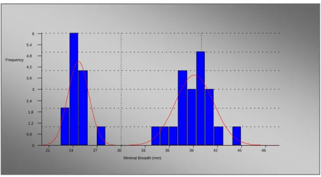
Figure 3b). Mixture Distribution of Minimal Breadth of the 1st phalanx (from fossil sites) dimensions as a
test case. 21 24 27 30 33 36 39 42 45 48 Minimal Breadth (mm) 0 0.6 1.2 1.8 2.4 3 3.6 4.2 4.8 5.4 6 Frequency
26 30 33 36 39 42 45 48 51 54 57 M axim un height (m m ) 0 0.5 1 1.5 2 2.5 3 3.5 4 4.5 F re q u e n cy
Figure 4: Mixture Distribution of Maximum height of 3rd phalanx dimensions.
2.1.2. 3rd Phalanx Anterior
Table 4: Results of mixture analysis of 3rd phalanx anterior of fossil horse
Variable M1 M2 P1 P2 SD1 SD2 Length 57.45 51.03 0.46 0.54 1.06 3.27 Ant. Length 57.33 43.70 0.70 0.30 2.27 1.70 Arti. Depth 38.87 50.99 0.30 0.70 0.84 1.76 Max. height 38.74 24.17 0.70 0.30 3.30 1.31 Angle 46.61 32.17 0.70 0.30 3.63 0.54 circumference 175.43 129.33 0.70 0.30 6.86 1.25
The following observations can be made regarding the results presented in Table 4.
a) Again one should say that Length is not a good parameter for establishing a sex ratio between the populations.
b) The prior probabilities P1 and P2 showing the probability population of Male and female which is 70% and 30%.
c) The Sex ratio is 70% for Males and 30% for females.
d) The Variables of 3rd Phalanx anterior showing Bimodal Distribution and indicating large Sexual Dimorphism.
2.1.3. Talus
As Length did not show degree of sexual dimorphism so Applicant did not take Length as the Variable in Talus.
Table 5: Result of mixture analysis of Talus of fossil horse
Variable M1 M2 P1 P2 SD1 SD2 Max. diameter 51.26 69.52 0.26 0.74 1.61 2.32 Breadth Trochlear 23.40 33.08 0.25 0.75 0.93 1.45 Max. Breadth 49.27 70.57 0.25 0.75 1.64 2.77 DA Breadth 59.49 43.65 0.75 0.25 2.90 1.35 DA Depth 39.29 30.02 0.75 0.25 1.33 0.97 Max depth 58.17 42.95 0.72 0.28 1.68 2.59
The following observations can be made regarding the results presented in Table 5.
a) The Prior probabilities P1 and P2 Showing the Sex ratio which is 75% and 25% approximately.
b) The two variables (Maximum Diameter and Maximum Depth) did not show the same sex ratio, it does not mean that the sex ratio is not accurate, as data is from different sites so they don’t have equal number in the variables.
c) The Variables of Talus showing Bimodal Distribution and indicating large Sexual Dimorphism.
28
42 45 48 51 54 57 60 63 66
D ist al A rt icular B readth (m m) 0 0.6 1.2 1.8 2.4 3 3.6 4.2 4.8 5.4 6 Fr e quenc y
Figure 5: Mixture Distribution of Maximum height of Talus from the fossil sites dimensions.
2.1.4. Calcaneus:
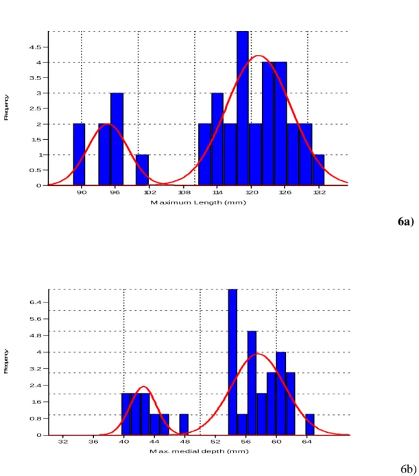
Table 6: Result of mixture analysis of Calcaneus of fossil horse.
Variable M1 M2 P1 P2 SD1 SD2 Max. length 121.29 94.53 0.77 0.23 5.69 3.55 Max.Diameter 62.18 84.18 0.23 0.77 1.99 3.75 Breadth troch 16.02 23.04 0.20 0.80 0.59 1.65 Max. breadth 27.08 35.50 0.18 0.82 0.81 3.31 DA Breadth 41.74 56.04 0.23 0.77 1.87 3.25 DA Depth 43.21 59.21 0.23 0.77 2.48 2.55 Max. Depth 42.43 57.61 0.23 0.77 1.75 3.51
The following observations can be made regarding the results presented in Table 6.
a) The Prior probabilities P1 and P2 Showing the Sex ratio which is 77% and 23% approximately.
b) The two variable (Maximum Breadth and Trochlear Breadth) did not show the same sex ratio, it does not mean that the sex ratio is not accurate or they are not good parameter for establishing sex ration, it because of unequal number in the variables.
c) The Variables of Calcaneus showing Bimodal Distribution and indicating large Sexual Dimorphism.
d) The interesting thing in this skeletal part that Maximal length is showing the same sex ratio which other is showing, it means may be in Calcaneus Maximum length can show some degree of sexual dimorphism.
90 96 102 108 114 120 126 132 M aximum Lengt h (mm ) 0 0.5 1 1.5 2 2.5 3 3.5 4 4.5 Fr equenc y 6a) 32 36 40 44 48 52 56 60 64
M ax. m edial dept h (m m ) 0 0.8 1.6 2.4 3.2 4 4.8 5.6 6.4 F re q u e n cy 6b)
30 b) Mixture Distribution of Maximum medial depth of Calcaneus dimensions.
2.1.5. Humerus
Table 7: Result of mixture analysis of Humerus of fossil horse.
Variable M1 M2 P1 P2 SD1 SD2 Max. Length 299.88 275.50 0.78 0.22 5.67 2.50 MLC 260.45 279.64 0.22 0.78 2.50 5.82 Mini. Breadth 31.04 38.50 0.22 0.78 2.05 1.16 Diameter 42.34 49.48 0.22 0.78 1.92 1.81 PMB 86.07 98.47 0.21 0.79 2.90 3.30 MBT 80.56 64.47 0.75 0.25 4.48 0.86 DMD 73.66 90.11 0.33 0.67 2.87 3.94 MTH 48.78 40.00 0.75 0.25 2.14 0.96 Mini. TH. 37.51 31.13 0.75 0.25 1.33 0.62 TH. 46.21 38.55 0.75 0.25 2.02 1.01
The following observations can be made regarding the results presented in Table 7.
a) The Prior probabilities P1 and P2 Showing the Sex ratio which is 78%-75% to 25% - 22% approximately.
b) Again in this skeletal part also Maximum length is showing the same sex ratio which other is showing approximately, it means may be in Humerus, Maximum length can show some degree of sexual dimorphism.
c) The Variables of Humerus showing Bimodal Distribution and indicating large Sexual Dimorphism.
d) Here there are two opinions about the sex ratio, some of the variables showing probability in Population between75% and 25% and some of the variables showing probability in population between 78% and 22%. This difference because of disequilibrium between the numbers of the variables.
e) The minimal Trochlear height is showing, which is not too longer in Size also showing large sexual dimorphism.
30 31.2 32.4 33.6 34.8 36 37.2 38.4 39.6 M inim al Tro c hlear height (m m )
0 1 2 3 4 5 6 7 8 F re q u e n cy
Figure 7: Mixture Distribution of Minimal Trochlear height of Humerous from the fossils sites dimensions.
2.1.6. Upper teeth
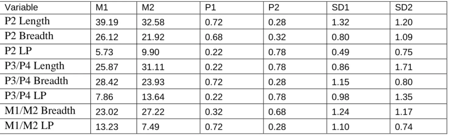
Table 8: Result of mixture analysis of the Upper teeth of fossil horse.
Variable M1 M2 P1 P2 SD1 SD2 P2 Length 39.19 32.58 0.72 0.28 1.32 1.20 P2 Breadth 26.12 21.92 0.68 0.32 0.80 1.09 P2 LP 5.73 9.90 0.22 0.78 0.49 0.75 P3/P4 Length 25.87 31.11 0.22 0.78 0.86 1.71 P3/P4 Breadth 28.42 23.93 0.72 0.28 1.15 0.80 P3/P4 LP 7.86 13.64 0.22 0.78 0.98 1.35 M1/M2 Breadth 23.02 27.22 0.32 0.68 1.24 1.17 M1/M2 LP 13.23 7.49 0.72 0.28 1.10 0.74
The following observations can be made regarding the results presented in Table 8.
a) The Prior probabilities P1 and P2 Showing the Sex ratio which is 68%-72% to 32% - 28% approximately.
32
b) Again in Upper Teeth also length of 2nd Premolar and 3rd /4th Premolar is showing the same sex ratio which other is showing approximately, it means may be in Upper Teeth, length can show some degree of sexual dimorphism.
c) In the table 7 there are two opinions about the sex ratio, some of the variables showing probability in Population between72% and 28% and some of the variables showing probability in population between 68% and 32%. These differences are because of unequalness between the numbers of the variables.
d) The Variables of Upper Teeth showing Bimodal Distribution, not too perfect like others skeletal part and indicating relatively less Sexual Dimorphism than others.
e) Moderately occlusal length of Premolar and molar length, Occlusal length of Protocone is indicating more sexual dimorphism.
8a) 4.8 5.6 6.4 7.2 8 8.8 9.6 10.4 11.2 P2 Length of Protocone (mm) 0 1.6 3.2 4.8 6.4 8 9.6 11.2 12.8 Frequency
21.6 22.8 24 25.2 26.4 27.6 28.8 30 31.2 P 3/ P 4 B readt h (mm ) 0 0.8 1.6 2.4 3.2 4 4.8 5.6 6.4 7.2 8 F requenc y 8b)
Figure 8: a) Mixture Distribution of 2nd Premolar height of the upper teeth from the fossil horses. b) Mixture Distribution of the Breadth of 3rd/ 4th Premolar of the Upper teeth from the fossil horses.
2.1.7. Mixture analysis of Geometric Mean:
After applying Mixture analysis there is bit difference in sex ratio, so applicant used geometric mean of all the above used variables. Applicant used geometric mean as a tester to check the accuracy of Sex ratio. Now the Question can be raised that what is geometric mean? Why Geometric mean used here?
The Geometric mean, in mathematics, is a type of mean or average, which indicates the central tendency or typical value of a set of numbers.
34
The geometric mean of the variables [(Var1*Var2* . . . *Varn)1/n] as a expression of the size (Mosiman, 1970). That is why applicant used geometric mean here as a tester. Rather using different variables, we used geometric mean of all skeletal part and analyze the Sex ratio.
Table 9: Result of Mixture Analysis of the Geometric mean of given variables.
Variable M1 M2 P1 P2 SD1 SD2 Upper Teeth 21.34 17.25 0.72 0.28 0.75 0.64 Calcanium 55.49 41.20 0.75 0.25 2.51 1.24 Astragulus 54.13 39.95 0.75 0.25 2.09 0.66 3rd Phalanx Anterior 45.00 61.04 0.30 0.70 1.22 1.91 3rd Phalanx Posterior 37.71 54.38 0.68 0.32 0.99 1.79 1st Phalanx Anterior 47.70 34.35 0.61 0.39 2.18 1.35 1st Phalanx Posterior 38.54 51.71 0.39 0.61 1.45 2.29
The following observations can be made regarding the results presented in Table 9.
a) The sex ratio almost the same as have shown in the above skeletal part separately.
b) There are three group of sex ratio between the population of fossil horse, it means the same that all variable have unequal numbers of population.
c) All the variable showing bimodal distribution and indicating large sexual dimorphism.
d) The sex ratio is varying from 61%-75% to 39%-25%.
2.2. Results for Changes in Size and Shape by Principal Component Analysis:
After the application of mixture analysis, we applied Principal component Analysis method to see the changes occur in Size and Shape. First we have analyzed Size and then Shape. In the process first we take out the percentage of variability and then load the Principal components. Applicant denoted Eisenmann data by Equus caballus(Eisenmann data 1) and Equus przewalskii (Eisenmann data 2).
2.2.1. Talus Size
Table 10: Eigenvalues and % of Variance and PC1 & PC2.
The following observations can be made regarding the results presented in Table 10.
a) First Principal Component (PC1) represents 96.26% of the total of the inertia explaining the variability of behaviours, which is really high, and clearly shows that PC1 is showing Size component.
b) In PC1 all the variables are highly negatively correlated each other, means they are bigger in size in the negative axis and smaller in size in the positive axis.
c) In PC2 only 1.33% showing variability, which is very less and may be negotiable, because of that Applicant didn’t use it for Explaining the Second Principal Component
2.2.1.1Talus Shape
Table 11: Eigenvalues and % of Variance and PC1 & PC2.
PC Eigenvalue % Variance 1 5.78 96.26 2 0.08 1.33 3 0.06 1.07 4 0.05 0.86 5 0.02 0.38 6 0.01 0.11 Variable PC 1 PC 2 Maxlength ‐0.99 0.14 MaxDiameter ‐0.99 0.11 Maxbreadth ‐0.98 ‐0.18 DABreadth ‐0.98 ‐0.11 DADepth ‐0.97 ‐0.01 MaxmDepth ‐0.98 0.02 PC Eigenvalue % Variance 1 2.39 39.85 2 1.43 23.75
36
The following observation can be made regarding the results presented in table 11.
a) First Principal Component (PC1) represents 39.85% of the total of the inertia explaining the variability of behaviours, which is quite good in numbers. The Jollife cut off is 0.7 so one will count first three Principal Component.
b) In the PC1 there will be high values of Maximum Length and Maximum diameter in the negative axis and low values in the positive axis, while Maximum Breadth and Distal Articular breadth have high values in positive axis, and low values in Negative Axis.
c) In PC2 Distal Articular Depth and Maximal Medial depth have high values in Negative axis while Distal Articular Breadth has high value in positive axis and vise- versa.
d) In the PC3Maximal medial depth has high value in negative Axis while distal articular depth has high value in positive axis and vise- versa.
3 1.21 20.21 4 0.69 11.50 5 0.27 4.48 6 0.01 0.21 Variable PC 1 PC 2 PC 3 Maxlength ‐0.89 0.10 0.15 MaxDiameter ‐0.83 0.44 ‐0.03 Maxbreadth 0.71 0.26 ‐0.34 DABreadth 0.55 0.65 0.10 DADepth 0.29 ‐0.55 0.77 MaxmDepth ‐0.11 ‐0.66 ‐0.68
9a)
9b
Figure 9: Principal component analysis of Astragulus a) showing variability in size; b) showing variability in
shape.
38
Table 12: Eigenvalues and % of Variance and PC1 & PC2.
PC Eigenvalue % Variance 1 6.44 91.99 2 0.19 2.69 3 0.12 1.76 4 0.08 1.21 5 0.07 0.96 6 0.05 0.77 7 0.04 0.63
The following observations can be made regarding the results presented in Table 12.
a) First Principal Component (PC1) represents 91.99% of the total of the inertia explaining the variability of behaviours, which is really high, and clearly one can say that PC1 is showing Size component.
b) In PC1 all the variables are highly negatively correlated each other, means they are bigger in size in the negative axis and smaller in size in the positive axis.
c) In PC2 only 2.69% showing variability, which is very less and may be neogiable, because of that Applicant didn’t use it for Explaining the Second Principal Component.
2.2.2.2. Calcaneus Shape
Table 13: Eigenvalues and % of Variance and PC1, PC2, PC3 & PC4.
PC Eigenvalue % Variance 1 1.87 26.77 2 1.37 19.64 3 1.17 16.76 4 1.07 15.24 5 0.82 11.70 6 0.68 9.76 7 0.01 0.13 Variable PC 1 PC 2 MaxLength ‐0.96 0.20 LengthProx. ‐0.96 0.19 MinBreadth ‐0.95 ‐0.10 PMB ‐0.93 ‐0.31 PMD ‐0.97 ‐0.02 DMB ‐0.97 ‐0.03 DMD ‐0.96 0.05 Variable PC 1 PC 2 PC3 PC4 MaxLength ‐0.77 0.04 0.12 0.07 LengthProx. ‐0.79 ‐0.15 ‐0.11 ‐0.06 MinBreadth 0.50 0.01 ‐0.79 ‐0.25 PMB 0.57 ‐0.06 0.72 ‐0.20 PMD 0.27 0.13 ‐0.05 0.95 DMB 0.11 ‐0.81 0.03 ‐0.05 DMD 0.00 0.82 0.07 ‐0.23
The following observation can be made regarding the results presented in table 13.
a) First Principal Component (PC1) represents 26.77% of the total of the inertia explaining the variability of behaviours, which is not bad in numbers. The julliffie cut off is 0.7 still applicants will count first four Principal Component.
b) In PC 1 Maximal length and length of the proximal part have high values in negative axis while Minimal breadth and proximal maximal breadth has high values in the positive axis and vise- versa.
c) In PC 2 Distal maximal breadth has high value in negative axis, while distal proximal depth has high value in positive axis and vise- versa.
d) In PC 3 Minimal Breadth has high value in negative axis, while proximal maximal breadth has high value in positive axis and vise- versa.
e) In PC 4 Proximal maximal depth will has high value, but it is univeriate, means proximal Maximal depth showing high values in positive axis, and vise- versa.
40
10a)
10b)
Figure 10: Principal component analysis of Calcanium a) showing variability in size; b) showing variability in
shape.
Table 14: Eigenvalues and % of Variance and PC1 & PC2. PC Eigenvalue % Variance 1 10.22 92.93 2 0.23 2.10 3 0.18 1.64 4 0.11 0.99 5 0.09 0.84 6 0.06 0.57 7 0.05 0.43 8 0.02 0.18 9 0.02 0.15 10 0.01 0.14 11 0.00 0.04
The following observations can be made regarding the results presented in Table 14.
a) First Principal Component (PC1) represents 92.93% of the total of the inertia explaining the variability of behaviours, which is really high, and clearly one can say that PC1 is showing Size component.
b) In PC1 all the variables are highly negatively correlated each other, means they are bigger in size in the negative axis and smaller in size in the positive axis.
c) In PC2 Diameter is Univeriate, but it will show high value in negative axis and low value in positive axis.
2.2.3.3. Humerus Shape:
Table 15: Eigenvalues and % of Variance and PC1, PC2, PC3 & PC4.
Variable PC 1 PC 2 Maxlength ‐0.98 0.11 MLC ‐0.97 0.13 MiniBrea ‐0.96 ‐0.11 Diameter ‐0.91 ‐0.40 PMB ‐0.98 0.00 PDMT ‐0.99 0.07 MBT ‐0.98 0.02 DMD ‐0.99 0.08 MTH ‐0.96 0.00 MiniTH ‐0.97 0.11 Trochheight ‐0.92 ‐0.05