Modelling and mapping aboveground biomass for energy usage and carbon storage assessment in mediterranean ecosystems

(1)

MODELLING AND MAPPING ABOVEGROUND

BIOMASS FOR ENERGY USAGE AND CARBON

STORAGE ASSESSMENT IN MEDITERRANEAN

ECOSYSTEMS

DOCTORAL DEGREE IN AGRICULTURAL AND FORESTRY

SCIENCES

Supervisor: Professor Doutor José Tadeu Marques Aranha

UNIVERSIDADE DE TRÁS-OS-MONTES E ALTO DOURO

(2)

(3)

Este trabalho foi expressamente elaborado como tese original com o objectivo da obtenção do grau de Doutor em Ciências Agronómicas e Florestais ao abrigo do Decreto-Lei n.º 74/2006, de 24 de Março, alterado pelo Decreto-Lei n.º 107/2008, de 25 de Junho, e pelo Decreto-Lei n.º 230/2009, de 14 de Setembro.

(4)

(5)

Acknowledgments

These lines that often go unnoticed to readers are perhaps the most complex to write. Given the dynamics involved in a task of this nature, as well the extended period of time for its realization, there were many people who, somehow, gave their contribution. Some people who were important in the beginning were replaced by others during the work. However, whether it was directly about the work, whether it was indirectly about several issues which are part of the individual, all contributions were important. So, my first thanks generic and abstract go to all those who, at some point, gave me encouragement to continue and go further.

In order to express adequately my gratitude to some people who gave me support during my research studies and made this thesis possible, the next lines will be written in Portuguese.

Ao Prof. Doutor José Aranha (Departamento de Ciências Florestais e Arquitectura Paisagista, Escola de Ciências Agrárias e Veterinárias da Universidade de Trás-os-Montes e Alto Douro), pela orientação, apoio, revisão de trabalhos e pela amizade que sempre emprestou nos momentos difíceis, e nos muito difíceis, que existiram ao longo destes vários anos.

Ao Prof. Doutor Domingos Lopes (Departamento de Ciências Florestais e Arquitectura Paisagista, Escola de Ciências Agrárias e Veterinárias da Universidade de Trás-os-Montes e Alto Douro), pela co-orientação no âmbito da bolsa da Fundação para a Ciência e a Tecnologia, que em dado momento foi cirúrgica para continuar o percurso, pelo incentivo, motivação, estabelecimento de pontes, cedência de contactos e amizade prestada.

Ao Prof. Doutor Warren B. Cohen (USDA Forest Service) pela co-orientação no âmbito da bolsa da Fundação para a Ciência e a Tecnologia, pela ajuda na revisão de trabalhos e por ter sido co-autor de artigos científicos publicados.

Ao Prof. Doutor José Luís Lousada (Departamento de Ciências Florestais e Arquitectura Paisagista, Escola de Ciências Agrárias e Veterinárias da Universidade de Trás-os-Montes e Alto Douro), pela ponte criada com a Escuela Universitaria de

(6)

Ingeniería Técnica Forestal da Universidade de Vigo, pelo auxílio na medição das densidades das amostras de biomassa e por ter sido co-autor de um artigo científico publicado.

Ao Prof. Doutor Luis Ortiz Torres (Escuela Universitaria de Ingeniería Técnica Forestal. Universidade de Vigo) por me ter recebido em Pontevera-Vigo e por ter sido co-autor de um artigo científico publicado.

Ao Doutor Daniel Vega-Nieva (Escuela Universitaria de Ingeniería Técnica Forestal. Universidade de Vigo), pela estreita colaboração enquanto co-autor de um artigo científico publicado.

Ao Prof. Doutor Carlos Pacheco Marques (Departamento de Ciências Florestais e Arquitectura Paisagista, Escola de Ciências Agrárias e Veterinárias da Universidade de Trás-os-Montes e Alto Douro) por ter tido a amabilidade de fazer uma recomendação para obtenção de uma bolsa de investigação científica.

Ao Investigador Doutor Paulo Fernandes (Departamento de Ciências Florestais e Arquitectura Paisagista, Escola de Ciências Agrárias e Veterinárias da Universidade de Trás-os-Montes e Alto Douro) por ter tido a amabilidade de fazer uma recomendação para obtenção de uma bolsa de investigação científica, pela cedência de bibliografia e por ter sido co-autor de um artigo publicado.

Ao Prof. Doutor Salvador Malheiro (Departamento de Engenharias, Escola de Ciências e Tecnologia da Universidade de Trás-os-Montes e Alto Douro), pela disponibilização de meios para medição dos poderes caloríficos das amostras de biomassa.

Ao Eng.º Cristóvão Santos (Departamento de Engenharias, Escola de Ciências e Tecnologia da Universidade de Trás-os-Montes e Alto Douro), pela sempre pronta ajuda e pelos ensinamentos que permitiram avaliar os poderes caloríficos das amostras de biomassa.

(7)

Ao Sr. Armindo Teixeira, assistente operacional do Laboratório de Produtos Florestais (Departamento de Ciências Florestais e Arquitectura Paisagista, Escola de Ciências Agrárias e Veterinárias, UTAD), pela ajuda e aconselhamento na preparação das amostras de biomassa para posterior análise termo-físico-químicas.

Às diversas empresas florestais que fizeram os abates dos pinheiros e eucaliptos agradeço terem acolhido, colaborado e permitido que se fizessem as medições de campo e pesagens da biomassa florestal.

Aos alunos e estagiários, hoje Licenciados, Bruno Abrantes, José Rocha, Henrique Silva, Carlos Carvalho e Mauro Santos, que parcialmente, em maior ou menor grau, foram participando nos fastidiosos trabalhos de campo como a medição, pesagem e separação das componentes de biomassa. Aos alunos e estagiários, hoje Licenciados, Carla Marques, Sara Dias, Ângelo Correia, Marco Cruz, Rogério Queirós, Ricardo Correia, que para além do maior volume de trabalho de campo colaboraram nas análises laboratoriais dos parâmetros termo-físico-químicos. A base de dados recolhida, que foi o cerne deste trabalho, não teria sido possível construir sem esta preciosa colaboração.

Ao Eng.º Rui Rocha da LECO Instrumentos, S.A., pela ajuda na avaliação química elementar das amostras de biomassa.

Ao Sr. Carlos Matos, técnico assistente, (Departamento de Química da Universidade de Trás-os-Montes e Alto Douro), pela realização das análises químicas das amostras de biomassa.

Aos Revisores anónimos das revistas e dos encontros científicos, aos quais submetemos parte dos estudos realizados, agradecemos os comentários e sugestões que contribuíram para a redacção desta tese.

(8)

À Escola Superior Agrária de Viseu do Instituto Superior Politécnico de Viseu (ESAV-IPV) pela flexibilidade na elaboração dos horários de docência no decurso dos trabalhos de Doutoramento.

Ao Eng.º Edgar Santos, amigo de longa data pelo apoio, pela leitura e revisão do Inglês da tese.

Às minhas colegas (ESAV-IPV), e fundamentalmente amigas Dr.ª Ana Liza Oliveira, Dr.ª Carla Santos e Engª Daniela Costa, cujo esplendor de brilho estelar desvanece os dias de trovoada.

Ao Prof. Doutor José Luís Pereira (ESAV-IPV), colega e amigo, pelas sugestões de organização da tese.

Ao Doutor João Mesquita (ESAV-IPV), colega e amigo, pela leitura e revisão do Inglês de partes da tese.

Ao Eng.º Pedro Cardoso, colega e amigo, pela leitura e revisão do Inglês da tese.

Ao Eng.º João Paulo Gouveia (ESAV-IPV), colega e amigo, e Dr.ª Ana Marques agradeço o apoio na árdua jornada.

Ao Eng.º António José Almeida, pela amizade e terapêuticas horas de convívio.

A todos aqueles que de alguma forma contribuíram para a realização desta tese.

Por último, àqueles que em última instância, mesmo que em silêncio, estão sempre lá a desejar-nos o melhor, os meus avós, pais, irmãos, cunhadas e sobrinhos com um especial beijo à minha irmã Cláudia que me soube surpreender.

(9)

Support Funding

The research described in this thesis was financially supported by a grant, ref: SFRH/PROTEC/49626/2009, for the period 2009-2012, from the Portuguese Science and Technology Foundation (FCT/MCTES, Portugal) and Polytechnic Institute of Viseu (IPV) The financial support included the tuition fees and 50 % reduction of the teaching workload.

Apoios de impressão da Tese:

“Este trabalho é financiado por Fundos FEDER através do Programa Operacional Factores de Competitividade - COMPETE e por Fundos Nacionais através da FCT - Fundação para a Ciência e a Tecnologia no âmbito do projecto FCOMP-01-0124-FEDER-022692”.

Supervisor: Prof. Doutor José Tadeu Marques Aranha from Departamento de Ciências

Florestais e Arquitectura Paisagista da Universidade de Trás-os-Montes e Alto Douro.

Co-supervisor: Prof. Doutor Domingos Manuel Mendes Lopes from Departamento de

Ciências Florestais e Arquitectura Paisagista da Universidade de Trás-os-Montes e Alto Douro.

Co-supervisor: Prof. Doutor Warren B. Cohen from College of Forestry of Oregon

(10)

(11)

Abstract

Estimates of aboveground biomass stocks are essential for studying the ecosystems dynamics as carbon sinks and consequent role in mitigating climate change. This is particularly important in Mediterranean ecosystems, since it is widely recognized their greater vulnerability to prospective climate change. Moreover, due to efforts in fossil fuels replacement the use of biomass to energy purposes has been increasing. As a consequence, measurements of aboveground biomass and knowledge of biomass characteristics and properties are needed for achieving accurate estimates. In this context, a study was carried out in the main Portuguese forest ecosystems: Maritime pine (Pinus pinaster Aiton) and Eucalyptus (Eucalyptus globulus Labill.) stands and in shrubland areas. Within these ecosystems-types located in the North-Center region of Portugal an exhaustive field wok were conducted, since 2006, to collect the data used in this research.

By means of destructive sampling technique a specific system of additive nonlinear allometric equations was developed for estimating maritime pine and eucalyptus aboveground biomass stocks and a set of specific equations were established to predict the shrubland aboveground biomass. To spatially assess the aboveground biomass stocks of forest stands and shrubland in this characteristic region, different mapping approaches based in inventory data, remote sensing imagery and spatial predictions models were investigated and compared. Apart from other physical and chemical properties determinations, carbon content in tree biomass components and shrub pool was achieved showing that the ecosystems studied store important amounts of carbon. The fuelwood characteristics and biomass combustion properties of maritime pine, eucalyptus and main native woody shrub species were evaluated and the potential of forest biomass for energy production at industrial scale in Portugal was assessed.

The developed specific equation models in conjunction with the studied mapping techniques and with the values found in this research, inter alia, of carbon fraction of dry matter and heating values per tree component are an important contribute to estimate more accurately the carbon uptake and the energy potential of the studied ecosystems.

Key-Words: Additive equations, Biomass, Bioenergy, Carbon, Forest Inventory, GIS,

(12)

(13)

Resumo

A quantificação da biomassa dos espaços florestais é essencial para a investigação da dinâmica dos ecossistemas como sumidouro de carbono e consequente papel na mitigação das alterações climáticas. Este conhecimento é particularmente importante nos ecossistemas mediterrânicos, uma vez que é amplamente reconhecida a sua maior vulnerabilidade às previstas alterações climáticas. Adicionalmente, a utilização de biomassa para produção de energia tem vindo a aumentar nos últimos anos com o intuito de substituir o consumo de energia, proveniente de fontes fósseis não renováveis. Consequentemente, as avaliações de biomassa bem como o estudo das suas características e propriedades são necessárias para se atingiram estimativas o mais correctas possíveis.

Neste contexto, foi delineado um estudo, desde 2006, nas espécies mais representativas dos ecossistemas florestais de Portugal: o pinheiro-bravo (Pinus pinaster Aiton) e o eucalipto (Eucalyptus globulus Labill.), bem como nas espécies arbustivas lenhosas que compõem as áreas mais significativas de matorral. No Norte e Centro do país, foram instaladas parcelas de inventário onde se fizeram diversas medições dendrométricas e, utilizando o método destrutivo, foram feitas pesagens da biomassa aérea das espécies mencionadas. Por ajustamento simultâneo foram desenvolvidos dois sistemas de equações para estimativa da biomassa das componentes de pinheiro bravo e das componentes de eucalipto, observando a aditividade das estimativas das componentes individuais. Foram também desenvolvidas diversas equações para estimativa da biomassa de matorral utilizando diferentes variáveis independentes. Com o intuito de fazer a quantificação espacial da biomassa florestal foram investigados diferentes métodos de mapeamento, combinando dados de inventário florestal convencional, dados obtidos em imagens de satélite e modelos de predição espacial, incluindo a geoestatística.

A biomassa florestal e arbustiva foi caracterizada e as propriedades avaliadas por análises termo-físico-químicas. Desta forma, foi possível avaliar o carbono acumulado quer na biomassa das diferentes fracções da árvore, quer nas principais espécies arbustivas lenhosas características destes ecossistemas. Os resultados mostraram que os valores diferem da fracção de 50%, usualmente considerada em diversos estudos. Com a obtenção destes valores, é possível fazer estimativas mais precisas da acumulação de carbono e consequentes emissões de dióxido de carbono para a atmosfera.

(14)

A avaliação dos poderes caloríficos da biomassa das diferentes componentes de pinheiro-bravo, eucalipto e matos, permite avaliar com maior rigor o potencial desta biomassa para fins energéticos. O potencial da biomassa de pinheiro-bravo e eucalipto para produção de energia, em centrais de biomassa dedicadas, foi avaliado para Portugal. A análise mostrou que para suprir as necessidades previstas para os projectos em curso terão de ser consideradas outras fontes de combustível.

O conjunto de modelos alométricos desenvolvidos associados aos métodos de mapeamento investigados e às medições das fracções de carbono e poderes caloríficos específicos para cada componente das espécies de pinheiro-bravo, eucalipto, bem como para as arbustivas lenhosas, são um contributo para se obter com maior exactidão o carbono capturado e o potencial energético da biomassa dos principais ecossistemas florestais da região Norte e Centro de Portugal.

Palavras-Chave: Ajustamento simultâneo, Biomassa, Bioenergia, Carbono, Inventário

(15)

scientific manuscripts, book chapter and in conference proceedings, ordered in reverse chronological order of their writing.

Viana, H., Vega-Nieva, D., Ortiz Torres, L., Lousada, J., Aranha, J., 2012. Fuel characterization and biomass combustion properties of selected native woody shrub species from central Portugal and NW Spain. Fuel 102, 737-745. (JCR® IF5-year (cites in 2011): 3.791; Q1).

Viana, H., Aranha, J., Lopes, D., Cohen, W.B., 2012. Estimation of crown biomass of

Pinus pinaster stands and shrubland above-ground biomass using forest

inventory data, remotely sensed imagery and spatial prediction models. Ecological Modelling 226, 22-35. (JCR® IF5-year (cites in 2011): 2.714; Q2).

Viana, H., Lopes, D., Aranha, J., 2011. Assessment of Forest Aboveground Biomass Stocks and Dynamics with Inventory Data, Remotely Sensed Imagery and Geostatistics, in: Shaukat, S.S. (ed.), Progress in Biomass and Bioenergy Production. InTech, pp. 107-130. ISBN: 978-953-307-491-7.

Aranha, J., Calvão, A., Lopes, D., Viana, H., 2011. Quantificação da biomassa consumida nos últimos 20 anos de fogos florestais no Norte de Portugal. Info 26, 44-49.

Viana H.; Aranha J.; Lopes D., 2011. Dedicated Biomass Plants for Combined Heat & Power (CHP). The Portuguese National Strategy. 19th European Biomass Conference and Exhibition. ETA-Florence Renewable Energies. Berlin, Germany. June 6-10.

Viana, H., Cohen, W.B., Lopes, D., Aranha, J., 2010. Assessment of forest biomass for use as energy. GIS-based analysis of geographical availability and locations of wood-fired power plants in Portugal. Applied Energy 87, 2551-2560. (JCR® IF2011: 5.106; Q1).

(16)

Viana, H., Dias, S., Marques, C., Cruz, M., Lopes, D., Aranha, J., 2009. Estabelecimento de modelos alométricos para predição da biomassa aérea da

Pinus Pinaster. Actas do 6º Congresso Florestal Nacional. Ponta Delgada,

Açores. 6-9 Outubro., pp. 771-775.

Viana, H., Dias, S., Marques, C., Cruz, M., Lopes, D., Aranha, J., 2009. Estabelecimento de modelos alométricos para predição da biomassa aérea de

Eucalyptus globulus. Actas do 6º Congresso Florestal Nacional. Ponta Delgada,

Açores. 6-9 Outubro, pp. 765-770.

Viana, H., Fernandes, P., Rocha, R., Lopes, D., Aranha, J., 2009. Alometria, Dinâmicas da Biomassa e do Carbono Fixado em Algumas Espécies Arbustivas de Portugal 6º Congresso Florestal Nacional. Ponta Delgada, Açores. 6-9 Outubro, pp. 244-252.

Viana, H., Lopes, D., Aranha, J., 2009. Predição de biomassa arbustiva lenhosa empregando dados de inventário e o índice de diferença normalizada extraído em imagens Landsat 5 TM, ISPV Millenium. 37.

Helder Viana contributed with idea, method, and experimental work to all publications except the following, whose initial idea and method was from José Aranha: Aranha, J., Calvão, A., Lopes, D., Viana, H., 2011. Quantificação da biomassa consumida nos últimos 20 anos de fogos florestais no Norte de Portugal. Info 26, 44-49.

Reprints of scientific manuscripts were made with permission from the publisher Elsevier.

(17)

9.4. Results and discussion ... 279 9.5. Conclusions ... 283 References ... 285 10 Conclusions ... 291 11 Future work ... 295 Annexes ... 299 Annex A ... 301 Annex B ... 309 Annex B.1 ... 311 Annex B.2 ... 323 Annex C ... 333 Annex C.1 ... 335 Annex C.2 ... 351 Annex D ... 377 Annex E ... 385 Annex E.1 ... 387 Annex E.2 ... 399 Annex E.3 ... 409 Annex E.4 ... 417

(22)

(23)

List of Figures

Figure 1.1 - Annual carbon cycle (Average for the time period 2000-2005). ... 4

Figure 1.2 - Human Perturbation of the Global Carbon Budget. ... 7

Figure 1.3 - Global Terrestrial carbon balance simplified... 10

Figure 3.1 - Location of the maritime pine stands sampled for the data acquisition. ... 44

Figure 3.2 - Proportion of the maritime pine biomass tree components in the measured sample plots. ... 52

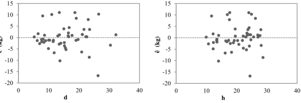
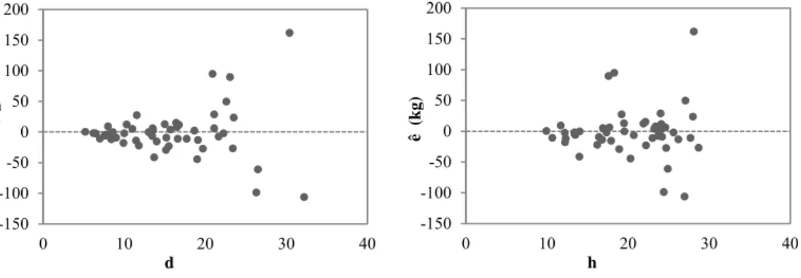
Figure 3.3 - Scatterplots of wood biomass residuals with the independent variables of the unweighted model. ... 60

Figure 3.4 - Scatterplots of bark biomass residuals with the independent variables of the unweighted model. ... 61

Figure 3.5 - Scatterplots of branches biomass residuals with the independent variables of the unweighted model. ... 61

Figure 3.6 - Scatterplots of needles biomass residuals with the independent variables of the unweighted model. ... 61

Figure 3.7 - Scatterplots of AGB biomass residuals with the independent variables of the unweighted model. ... 61

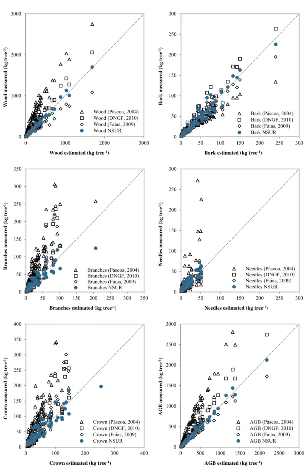
Figure 3.8 - Scatterplots of the measured versus predicted maritime pine biomass components fitted by the NSUR system. ... 66

Figure 3.9 - Scatterplots of the measured versus predicted maritime pine biomass components fitted by the NSUR system in the validation dataset. ... 68

Figure 3.10 - Scatterplots comparing the maritime pine biomass estimates from NSUR equation system and from equations adjusted by other authors. ... 71

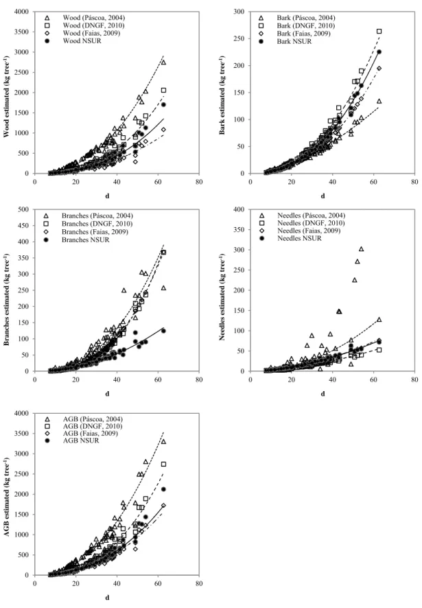
Figure 3.11 - Relationships between the maritime pine biomass estimates by the NSUR equations system and the diameter at breast height. ... 72

Figure 3.12 - Scatterplots comparing the maritime pine fresh biomass estimates from NSUR system and from equations adjusted by Barreto (2005). ... 73

(24)

Figure 3.13 - Scatterplots comparing the maritime pine crowns biomass estimates from NSUR equation system and from equations adjusted by OLS from other authors. ... 74

Figure 4.1 - Location of the eucalyptus sample plots. ... 87

Figure 4.2 - Proportion of the eucalyptus biomass tree components in the measured sample plots. ... 95

Figure 4.3 - Scatterplots of wood biomass residuals with the independent variables of the unweighted model. ... 101

Figure 4.4 - Scatterplots of bark biomass residuals with the independent variables of the unweighted model. ... 102

Figure 4.5 - Scatterplots of branches biomass residuals with the independent variables of the unweighted model. ... 102

Figure 4.6 - Scatterplots of leaves biomass residuals with the independent variables of the unweighted model. ... 102

Figure 4.7 - Scatterplots of top biomass residuals with the independent variables of the unweighted model. ... 103

Figure 4.8 - Scatterplots of AGB biomass residuals with the independent variables of the unweighted model. ... 103

Figure 4.9 - Scatterplots of the measured versus predicted eucalyptus biomass components fitted by the NSUR system. ... 107

Figure 4.9 - Scatterplots of the measured versus predicted eucalyptus biomass components fitted by the NSUR system (cont.). ... 108

Figure 4.10 - Scatterplots of the measured versus predicted eucalyptus biomass components fitted by the NSUR system in the validation dataset. ... 109

Figure 4.11 - Scatterplots comparing the eucalyptus biomass estimates from the NSUR equation system and from equations adjusted by other authors. ... 112

Figure 4.12 - Relationships between the eucalyptus biomass estimates by the NSUR equations system and the diameter at breast height. ... 113

(25)

Figure 4.13 - Scatterplots comparing the eucalyptus biomass estimates from the NSUR equation system and from the equations, adjusted by OLS from other authors. ... 114

Figure 5.1 - Location of the shrubland sample plots in the NUT III sub-regions. ... 126

Figure 5.2 - Burnt areas in Portugal from 1990 to 2007 and sample plots location. ... 127

Figure 5.3 - Occurrence of species in the measured sample plots in the Dão-Lafões region. ... 135

Figure 5.4 - Occurrence of species in the measured sample plots in Tâmega region. .. 136

Figure 5.5 - Occurrence of species in the measured sample plots in Serra da Estrela region. ... 136

Figure 5.6 - Scatterplots of the measured versus predicted shrubland aboveground biomass for the Dão-Lafões region. ... 143

Figure 5.7 - Scatterplots of the measured versus predicted shrubland aboveground biomass for the Tâmega region. ... 143

Figure 5.8 - Scatterplots of the measured versus predicted shrubland aboveground biomass for the Serra da Estrela region. ... 144

Figure 5.9 - Scatterplots of the measured versus predicted shrubland aboveground biomass for the Global data. ... 144

Figure 5.10 - Scatterplots of predicted shrubland aboveground biomass and independent variables. ... 146

Figure 5.11 - Scatterplots comparing the AGB measured versus the AGB estimated by equations from other authors. ... 147

Figure 6.1 - Higher heating values of biomass tree components (a) eucalyptus and (b) maritime pine. ... 175

Figure 7.1 - Higher heating values of shrub species for the two areas of study. ... 207

Figure 8.1 - Study area. ... 235

Figure 8.2 - Scatterplots of measured biomass versus estimated biomass from regression equations with NDVI as independent variable. ... 245

(26)

Figure 8.4 - Experimental omnidirectional semivariogram for pine biomass. ... 246

Figure 8.5 - Comparison of Root Mean Square Errors (RMSE). ... 248

Figure 8.6 - Spatially explicit AGB estimates (ton ha-1) for the study area generated from DRR spatial prediction method (a) pine stands (b) shrubland. ... 251

Figure 8.7 - Regression performed between DRR and RK Biomass maps. ... 252

Figure 9.1 - NUT III sub-regions. ... 271

Figure 9.2 - Power plants location with the identification of the NUT II sub-regions boundaries, and the optimum biomass supply area (R=35km). ... 278

Figure 9.3 - Logging residues availability at regional scale. ... 281

Figure 9.4 - Total theoretical and available (within a radius of 35Km) biomass potential supply. ... 282

(27)

List of Tables

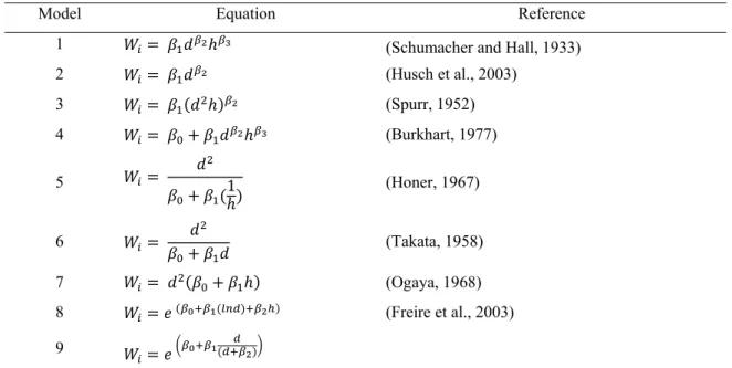
Table 3.1 - Best candidate models. ... 47

Table 3.2 - Descriptive statistics of maritime pine stands. ... 51

Table 3.3 - Statistics of the best fitted models to the wood stem biomass. ... 54

Table 3.4 - Statistics of the best fitted models to the bark stem biomass. ... 55

Table 3.5 - Statistics of the best fitted models to the top biomass. ... 56

Table 3.6 - Statistics of the best fitted models to the branches biomass. ... 57

Table 3.7 - Statistics of the best fitted models to the needles biomass. ... 58

Table 3.8 - Statistics of the best fitted models to the entire aboveground biomass... 59

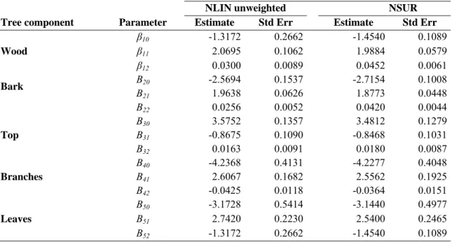
Table 3.9 - Parameter estimates and standard errors of the nonlinear unweighted models and of the NSUR system for fresh maritime pine biomass. ... 63

Table 3.10 - Parameter estimates and standard errors of the nonlinear unweighted models and of the NSUR system for air dried maritime pine biomass. ... 63

Table 3.11 - Parameter estimates and standard errors of the nonlinear unweighted models and of the NSUR system for oven dried maritime pine biomass. .... 64

Table 3.12 - Statistics of the fitted additive nonlinear simultaneous equations system. . 65

Table 3.13 - Statistics of the estimates obtained by NSUR System and equations from other authors. ... 70

Table 4.1 - Best candidate models to fit Eucalyptus biomass tree components. ... 90

Table 4.2 - Descriptive statistics of eucalyptus stands. ... 94

Table 4.3 - Statistics of the fitted models to the wood stem biomass... 96

Table 4.4 - Statistics of the fitted models to the bark stem biomass. ... 97

Table 4.5 - Statistics of the fitted models to the top biomass. ... 98

Table 4.6 - Statistics of the fitted models to the branches biomass. ... 98

Table 4.7 - Statistics of the fitted models to the biomass of leaves. ... 99

(28)

Table 4.9 - Parameter estimates and standard errors of the nonlinear unweighted models and of the nonlinear simultaneous system of fresh biomass. ... 104

Table 4.10 - Parameter estimates and standard errors of the nonlinear unweighted models and of the nonlinear simultaneous system of air dried biomass... 105

Table 4.11 - Parameter estimates and standard errors of the nonlinear unweighted models and of the nonlinear simultaneous system of oven dried biomass. 105

Table 4.12 - Statistics of the fitted additive nonlinear simultaneous biomass equation system. ... 106

Table 4.13 - Statistics of the estimates obtained by the equations from other authors. 111

Table 5.1 - Regression models fitted to predict the shrubland aboveground biomass. . 131

Table 5.2 - Equation models to estimate shrubland AGB in Mediterranean regions. ... 133

Table 5.3 - Descriptive statistics of the shrub species measured in the sample plots. .. 134

Table 5.4 - Characteristics of shrubs sampled in the three sites of study grouped by vegetation's age. ... 137

Table 5.5 - Statistics of the fitted models to predict the shrubland AGB in Dão-Lafões region. ... 138

Table 5.6 - Statistics of the fitted models to predict the shrubland AGB in Tâmega region. ... 139

Table 5.7 - Statistics of the fitted models to predict the shrubland AGB in Serra da Estrela region. ... 139

Table 5.8 - Statistics of the fitted models to predict the shrubland AGB for the Global dataset. ... 140

Table 5.9 - Parameter estimates and correction factors of the selected shrubland AGB models. ... 141

Table 5.10 - Evaluation of the fitted Global models using the data of each region as validation dataset. ... 145

Table 5.11 - Statistics of the estimates obtained by the equations from other authors. 149

Table 5.12 - One-Way ANOVA performed among shrubland aboveground biomass estimates. ... 150

(29)

Table 5.13 - Tukey HSD All-Pairwise Comparisons Test performed among shrubland AGB estimates. ... 150

Table 6.1 - Descriptive statistics of eucalyptus stands. ... 170

Table 6.2 - Descriptive statistics of maritime pine stands. ... 170

Table 6.3 - Proximate analysis and basic density of eucalyptus and maritime pine species. ... 171

Table 6.4 - Ultimate analysis of eucalyptus and maritime pine species. ... 173

Table 6.5 - Higher and lower heating values, Moisture content and Density of eucalyptus and maritime pine biomass components. ... 174

Table 6.6 - Higher and lower heating values, fuelwood value index and energy density.176

Table 6.7 - Concentrations (mg kg-1) of heavy metals in ash of Eucalyptus globulus and Pinus pinaster and limit values on European countries’ legislation. ... 179

Table 7.1 - Descriptive statistics of the shrub biomass sampling plots at the two areas of study. ... 202

Table 7.2 - Proximate analysis and basic density of the shrub species at the two areas of study. ... 204

Table 7.3 - Ultimate analysis of the shrub species at the two areas of study. ... 206

Table 7.4 - Higher and lower heating values and energy density of the studied shrub species. ... 207

Table 7.5 - Shrub ash major and selected minor elements composition. ... 209

Table 7.6 - Ash slagging and fouling indices and risk. ... 212

Table 7.7 - Shrub ash traces and selected minor elements composition. ... 213

Table 8.1 - Descriptive statistics of data measured in the inventory dataset. ... 242

Table 8.2 - Allometric equations used to estimate biomass in the field plots. ... 243

Table 8.3 - Regression models developed using stand-wise forest inventory data and Landsat 5 TM and MODIS image data. ... 244

Table 8.4 - Shrub and Pine AGB estimation models evaluation using the validation sample plots. ... 247

(30)

Table 8.5 - Results from ANOVA to compare the differences between the means of the different prediction methods. ... 248

Table 8.6 - Tukey HSD all-pairwise comparisons test. ... 249

Table 8.7 - Summary statistics of crown biomass of pine stands maps estimated from spatial prediction methods. ... 250

Table 8.8 - Summary statistics of shrub AGB maps estimated from spatial prediction methods. ... 250

Table 8.9 - Spatial Correlation coefficients calculated between pine crown biomass maps. ... 252

Table 8.10 - Spatial Correlation coefficients calculated between shrub AGB map estimates. ... 252

Table 9.1 - Allometric equations used to estimate the residual forest biomass of maritime pine stands. ... 273

Table 9.2 - Allometric equations used to estimate the residual forest biomass of eucalyptus stands. ... 273

Table 9.3 - Technical parameters for a wood fired plant... 276

Table 9.4 - Total amount of theoretical and available residual biomass from maritime pine and eucalyptus, by NUT II sub-region. ... 279

Table 9.5 - Potential power production of fully condensing plants and cogeneration plants. ... 283

(31)

1

Introduction

______________________________________

(32)

(33)

1.1 Climate change and Terrestrial Carbon Processes

Climate change, which discussion has been done worldwide, is recognized by the Intergovernmental Panel on Climate Change (IPCC, 2011) as one of the great challenges of the 21st century. The global response to climate change, started in 1992 with the United Nations Framework Convention on Climate Change (UNFCCC) (United Nations, 1992) and strengthened by the commitment established with the Kyoto Protocol, in 1997 (United Nations, 1998), formally recognized the need of reduce and prevent anthropogenic emissions of greenhouse gases (GHG), where the carbon dioxide (CO2) sequestration in marine and terrestrial ecosystems receive particular attention.

Terrestrial ecological systems, in which carbon is retained in live biomass, decomposing organic matter, and soil, play an important role in the global carbon cycle (IPCC, 2000a). The dynamics of terrestrial ecosystems depend on interactions between a number of biogeochemical cycles, particularly the carbon cycle, nutrient cycles, and the hydrological cycle, all of which may be modified by human actions (IPCC, 2000a).

The carbon cycle is the fluxes of carbon among four main reservoirs: fossil carbon, the atmosphere, the oceans, and the terrestrial biosphere (Figure 1.1). A wide range of direct and indirect measurements confirm that the atmospheric mixing ratio of CO2 has increased globally by 36%, from a range of 275 to 285 ppm (ppm = parts per

million) in the pre-industrial Era (usually dated from 1750) to 379 ppm in 2005, as concluded in the IPCC Fourth Assessment Report (AR4) (Forster et al., 2007), and continued to grow to over 390 ppm (39%) above pre-industrial levels, by the end of 2010 (IPCC, 2011). The annual growth rate of atmospheric CO2 was 2.36±0.09 ppm in

2010, one of the largest growth rates in the past decade. The average for the decade 2000-2009 was 1.9±0.1 ppm per year, 1.5±0.1 ppm for the decade 1990-1999, and 1.6±0.1 for the decade 1980-1989. The present concentration is the highest during at least the last 800,000 years (GCP, 2012). The accumulation of atmospheric CO2 in 2010

was 5.0±0.2 PgC (1 Pg = Petagram = 1Gigatonne = 1 billion metric tons = 1x1015 g), with a total cumulative of 157.5 PgC since the beginning of atmospheric high precision measurements in 1959 and 237 PgC since 1750.

(34)

Figure 1.1 - Annual carbon cycle (Average for the time period 2000-2005). Source: Adapted from PMEL Carbon Group (2012).

Note: The numbers in square brackets shows the pre-industrial carbon values storage plus the balance after the human emissions. The exchanges of CO2 between different pools of carbon indicate the effects

that the human emissions have had on the carbon cycle. The exchanges are in pentagrams of carbon per year (PgC yr-1_).

The rates of atmospheric CO2 accumulation are influenced by both the

anthropogenic emissions and the net uptake by natural sinks (ocean and land) (GCP, 2012). Hence, uncertainties in the individual numbers of carbon budget are large as it remains difficult to quantify the influences of the separate but interactive several processes (e.g. forest regrowth, CO2 fertilization of plant growth, the interaction with

other biogeochemical cycles) in the fluxes among the main carbon reservoirs (Schimel, 1995).

(35)

1.2 Fossil Fuel and Cement CO

2

Emissions

Among the many human activities that produce Greenhouse Gases, the use of energy represents by far the largest source of emissions. GHG emissions from the energy sector are dominated by the direct combustion of fuels. Since the Industrial Revolution, annual CO2 emissions from fuel combustion increased from near zero to

concerning values. The annual emission rate from fossil fuel burning (plus a small contribution from cement production) averaged 5.4 ± 0.3 PgC yr-1 during 1980 to 1989, 6.3 ± 0.4 PgC yr-1 during 1990 to 1999 (Prentice et al., 2001) and 7.2± 0.3 PgC yr-1 in 2000–2005 (IPCC, 2007b). However, the increasing rate of growth of CO2 emissions

averaged 7.9 PgC yr-1 (29 Pg CO2) in 2009 (IEA, 2011b) and in 2010 reached 9.1±0.5

PgC (33.4 Pg CO2)(Peters et al., 2012).

Accordingly IEA (2011b) statistics, CO2 from energy represents about 83% of

the anthropogenic GHG emissions for the Annex I countries of the United Nations Framework Convention on Climate Change and about 65% of global emissions (IEA, 2011b). Activities related to land-use, primarily tropical deforestation and biomass burning are responsible for the rest of the emissions. However, according to the rates of anthropogenic CO2 emissions reported, for 2010 (Boden et al., 2011; Peters et al.,

2012), 91% (9.1±0.5PgC yr-1; 33.4 Pg CO2) are due to fossil fuel and Cement burning

and 9% are due to land-use change (0.9±0.7 PgC yr-1; 3.3 Pg CO2) leading to total

emissions (including fossil fuel and land-use change) of 10.0±0.9 PgC yr-1. These differences and discrepancies in estimates of carbon emissions have been reported and analysed in order to understand how uncertain are estimates of CO2 emissions (e. g.

IPCC, 2000b; Houghton, 2003b; IPCC, 2006b; Marland et al., 2009). In general, the uncertainties of quantified emission are attributed to the uncertainties of statistics independently reported by the largest contributing organizations under the UNFCCC (UNFCCC, 2012) and the Kyoto Protocol, which depend on the quality and availability of sufficient data and comparable methods to estimate emissions (IEA, 2011b).

(36)

1.3 Land Use, Land-Use Change, and Forestry (LULUCF) on

Greenhouse Gas Sources and Sinks

Since the Kyoto Protocol (United Nations, 1998) that Land Use, Land-Use Change and Forestry (LULUCF) activities received special concern as one of the major sources and sinks of GHG emissions. According to the Kyoto Protocol, signatories countries (Annex I) are required to report afforestation, reforestation and deforestation since 1990 (Article 3.3). Parties can elect to report emissions and removals from any of the following other human-induced activities since 1990 (Art. 3.4): Forest Management, Cropland Management, Grassland Management and Re-vegetation. The methodologies to estimate emissions and removals of GHG are described in the methodological guidelines by IPCC (IPCC, 2003, 2006a), which will be addressed in section 1.6.

Changes in land use and management affect the amount of carbon in plant biomass and soils (Prentice et al., 2001). During the last two centuries, soils have lost a considerable amount of C due to land use changes and expansion of agriculture. These losses from soils are clearly of concern in relation to future productivity and environment (Nieder and Benbi, 2008). The uncertainty on Land Use, Land-Use Change, and Forestry (LULUCF) emissions is the highest of any flux component of the global carbon budget. Since in the past decades, the CO2 flux caused by land-use

changes has been dominated by tropical deforestation (Denman et al., 2007; Havemann, 2009), the large uncertainties in emission estimates arise from inadequate data on the carbon density of forests and the regional rates of deforestation (Baccini et al., 2012).

The average annual global carbon budgets for 1980–1989 and 1989-1998 were estimated in 1.7±0.8 PgC yr-1 and 1.6±0.8 PgC yr-1, respectively (IPCC, 2000a). For the period between 2000-2010 (Figure 1.2) the average rate of carbon emissions due to LULUCF account around 11% (1.0±0.7 PgC yr-1) as the fossil fuel rate are estimated in 89% (7.9±0.5 PgC yr-1_{) (Boden et al., 2011; Peters et al., 2012). However, different}

estimates of the land use flux than those reported in the Third Assessment Report (TAR) (Prentice et al., 2001) were updated for the 1980s and for the 1990s (2.0 ± 0.8 PgC yr-1 and 2.2 ± 0.8 PgC yr-1, respectively (Houghton, 2003a), which gives even more higher carbon losses from tropical deforestation (Denman et al., 2007). Although the uncertainty in the net CO2 emissions due to land-use change is large, the estimated net

emissions for the decade of 2000 reveal a decline trend from the emissions due to land-use change. Carbon losses occur through decreased vegetation productivity, increased

(37)

respiration, deforestation, biomass combustion and other poor land management practices. The implementation of new land policies, higher law enforcement to stop illegal deforestation, and new afforestation and regrowth of previously deforested areas could all have contributed to this decline (GCP, 2012).

Figure 1.2 - Human Perturbation of the Global Carbon Budget. Source: Adapted from Global Carbon Project (2012).

Accordingly the Global Forest Resources Assessment 2010 (FRA 2010) the afforestation and natural expansion of forests in some countries and regions have reduced the net loss of forest area significantly at the global level. The net change in forest area in the period 2000-2010 is estimated at -5.2 million hectares per year, down from -8.3 million hectares per year in the period 1990–2000. Additionally, during 2005-2010, the area of planted forest increased by about 5 million hectares per year (FAO, 2010a). In fact, during the last decades, terrestrial ecosystems may have served as a small net sink for CO2. This terrestrial sink seems to have occurred in spite of net

(38)

terrestrial carbon uptake, that approximately balances the emissions from land-use change in the tropics, results from land-use practices and natural regrowth in middle and high latitudes, the indirect effects of human activities (e.g., atmospheric CO2

fertilization and nutrient deposition), and changing climate (both natural and anthropogenic). It is presently not possible to determine the relative importance of these different processes, which also vary from region to region (IPCC, 2000a). Hence, understanding CO2 capture and storage as well how human activities change carbon

stocks in the main pools (fossil carbon, the atmosphere, the oceans, and the terrestrial biosphere) and exchanges between them through LULUCF, among other activities has been the focus of scientific research.

(39)

1.4 Role of forests in carbon capture and storage

Quantifying the substantial roles of forests as carbon stores, as sources of carbon emissions and as carbon sinks has become one of the keys to understanding and influencing the global carbon cycle (FAO, 2010a). The biosphere constitutes a carbon sink that absorbed about 2.5 ± 1.0 PgC yr-1 from 2000 to 2010 (Figure 1.2). However, the potential of carbon storage varies in the various terrestrial ecosystems (Pan et al., 2011). Forests play a major role in global carbon cycle because they cover around 31 per cent (over 4 billion hectares) of terrestrial lands (FAO, 2010a) and contain more carbon per unit area than any other land types, accounting for 60% of total of carbon in terrestrial vegetation (FAO, 2001). The Global Forest Resources Assessment (FRA) 2010 estimates that the world’s forests store more than 650 Gt of carbon, being that 286 Gt (44%) of carbon are captured in their biomass alone (FAO, 2010a). Furthermore, as soils are the largest carbon reservoir of the terrestrial carbon cycle (FAO, 2001, 2004, 2010a), forest soils are of major importance for carbon store, accounting for 292.5 (Gt) 45% of total of carbon soil pool. The remaining 11% is stored in dead wood and litter.

While sustainable management, planting and rehabilitation of forests can conserve or increase forest carbon stocks, deforestation, degradation and poor forest management reduce them. For the entire world, carbon stocks in forest biomass decreased by an estimated 0.5 Gt annually during the period 2005–2010, mainly because of a reduction in the global forest area (FAO, 2010a). Hence, enhancing carbon uptake through afforestation and sustainable forest management, and Reducing Emissions from Deforestation and Forest Degradation (REDD) (UN-REDD Programme, 2009) has been an effort measure to mitigate elevated atmospheric CO2

concentration.

Carbon sequestration rates vary depending on plant species, soil type, region, climate, topography and management practices that can affect plant productivity, so the carbon storage of forests may change substantially with forest ecosystems on a community scale (Van Der Valk, 2009). Carbon begins its cycle through forest ecosystems (Figure 1.3) when plants assimilate atmospheric CO2 through

photosynthesis and convert it to biomass (Klass, 1998; Nieder and Benbi, 2008). Usually about half the gross photosynthetic products produced (GPP) are expended by plants in autotrophic respiration (Ra) for the synthesis and maintenance of living cells, releasing CO2 back into the atmosphere. The remaining carbon products (GPP - Ra) go

(40)

into net primary production (NPP): foliage, branches, stems, roots, and plant reproductive organs (Waring and Running, 2007). Annual primary production (NPP) represents the net amount of carbon sequestered into dry matter during a year (Melillo et al., 1993; Roy and Saugier, 2001) and is equivalent to total carbon uptake through photosynthesis minus the loss through autotrophic respiration. At the local scale, NPP can be defined and measured in terms of either biomass or CO2 exchange, though

measurements based on biomass data are by far the most common (Field et al., 1995). In practice, NPP is estimated by summing the growth of all tissue (change in live biomass plus litter) produced during a year (Waring and Running, 2007).

Biomass can be defined as the total amount of live and inert organic matter aboveground and belowground in a particular ecosystem. Changes in time of the quantity of biomass per unit area (biomass density) are a direct measure of carbon sequestration or loss between terrestrial ecosystems and the atmosphere. Thus, it can be used to determine the amount of carbon emitted to the atmosphere (as CO2, CO, and

CH4 through burning and decay) when ecosystems are disturbed (Houghton et al.,

2009). Therefore, a global assessment of biomass and its dynamics is an essential input to climate change forecasting models and mitigation and adaptation strategies (e.g. GTOS, 2009; GCOS, 2011).

Figure 1.3 - Global Terrestrial carbon balance simplified. Source: Adapted from IPCC (2000a).

Note: Plant (autotrophic) respiration releases CO2 to the atmosphere, reducing GPP to NPP and resulting

in short-term carbon uptake. Decomposition (heterotrophic respiration) of litter and soils in excess of that resulting from disturbance further releases CO2 to the atmosphere, reducing NPP to NEP and resulting in

medium-term carbon uptake. Disturbance from both natural and anthropogenic sources (e.g., harvest) leads to further release of CO2 to the atmosphere by additional heterotrophic respiration and

(41)

1.5 Biomass energy and climate change

As previous mentioned, recent data confirm that consumption of fossil fuels resulting from the provision of energy services accounts for the majority of global anthropogenic GHG emissions, with over 90% in 2010, (Peters et al., 2012). In order to mitigate GHG emissions from the energy system while still satisfying the global demand for energy services, several possible options were assessed in the IPCC Fourth Assessment Report (AR4) (IPCC, 2007a). These options includes carbon capture and storage (CCS) and Renewable Energy (RE) as reviewed in the IPCC Special Report on Renewable Energy Sources and Climate Change Mitigation (SRREN) (IPCC, 2011). A particular emphasis has been given to Bioenergy since a variety of biomass feedstocks, including forest, agricultural and livestock residues; short-rotation forest plantations; energy crops; the organic component of municipal solid waste; and other organic waste streams can be directly used to produce electricity or heat, or can be used to create gaseous, liquid, or solid fuels. Highlights of the most significant developments and perspectives of the bioenergy sector can be consulted in several recent reports (e.g. Bogdanski et al., 2011; European Commission, 2011a; GBEP, 2011; IEA, 2011a; IPCC, 2011).

On a global basis, it is estimated that of the total 492 Exajoules (EJ)of primary energy supply in 2008 RE accounted for 12.9% where the biomass contributed with 10.2%. A first qualitative understanding of biomass technical potentials can be gained from considering the total annual aboveground net primary production (NPP) on the Earth’s terrestrial surface. This is estimated to be about 35 Gt carbon, or 1,260 EJ yr-1, assuming an average carbon content of 50% and 18 GJ ton-1 average heating value. Comparing with the world primary energy supply of about 500 EJ yr-1 in 2009 (IEA, 2011b) total terrestrial aboveground NPP is larger than what is required to meet society’s energy demand (IPCC, 2011).

Despite the technical potentials and factors such as sustainability, concerns public acceptance, system integration and infrastructure constraints, or economic factors could limit to the continued growth of some individual RE technologies they continue to have significant opportunities for increased deployment (IPCC, 2011). In the case of energy production from biomass, the potential is recognized (e.g. Klass, 1998; Hakkila and Parikka, 2002; IEAGHG, 2011) and several policies are being adopted, leading to the development of new and safer energy sources, thus contributing to reducing

(42)

dependence on fossil fuels and the consequent reduction of GHG emissions. The European Union (EU) has been a pioneer in taking effective steps on promoting biomass energy, having started from the 90's a strategy on climate and energy (Commission of the European Communities, 1996; European Commission, 1997, 2001b, 2001a; Commission of the European Communities, 2005, 2008b, 2008a; European Parliament, 2009; European Commission, 2011b, 2011a). As result, EU member countries with forest resources have been implementing several projects for energy production (Combined Heat and Power, CHP) from biomass (e.g. Viana et al., 2010).

Biomass is generally indicated as having no net release of CO2 or “carbon

neutral” meaning that carbon emitted by biomass burning for power won’t contribute to climate change. It is assumed that if biomass is harvested and subsequently regrows without an overall loss of carbon stocks, there would be no net CO2 emissions over a

full harvest/growth cycle. In this way, land can be used continuously for the production of biomass energy to avoid fossil fuel CO2 emissions. By contrast, using land to grow

carbon stocks to be conserved thereafter can only be a temporary measure to limit fossil fuel use (IPCC, 2000a). However, this issue is not consensual as the CO2 emissions

released in the growth, harvest and transport the biomass for use as a fuel source are not accounted to the carbon footprint of biomass (e.g. Johnson, 2009; Biomass Energy Resource Center et al., 2012). The need to include land use and land-use change emissions of the biomass energy system in the GHG emission balances had already been identified by the IPCC Special Report of LULUCF of (IPCC, 2000a). Broad agreement about the advantages of biomass energy can be achieved in the future, with the view of the development of technologies to the carbon capture and storage emissions from biomass combustion (see Kraxner et al., 2003; IPCC, 2005; Biorecro AB and Global CCS Institute, 2010). These technologies, known as Bio-energy with carbon capture and storage (BECCS), could achieve a permanent net removal of CO2

from the atmosphere, or negative CO2 emissions (IEAGHG, 2011; IEA, 2012).

The use of forest biomass as an alternative, or complement, to the conventional energy sources can contribute to meeting our energy needs, and so pressure reduction on the consumption of fossil fuels accomplishing the recognized positive effects in the climate change.

(43)

1.6 Measuring aboveground forest biomass

Accurate quantitative estimation of forest biomass, expressed in terms of dry weight of living organisms, is important for analysing ecosystem productivity and also for assessing energy potential and the role of forests in the carbon cycle (FAO, 2010a).

As result of the UNFCCC (United Nations, 1992) and the Kyoto Protocol (United Nations, 1998) all member countries should assess and report national GHG emissions regularly. Emissions or removals of CO2 in the LULUCF (IPCC, 2003) sector

are estimated on the basis of changes of carbon stocks in the different pools (above-ground and below-(above-ground biomass; dead organic matter as dead wood and litter; and soil organic matter). Generally, the aboveground biomass comprise all biomass of living vegetation, both woody and herbaceous, above the soil including stems, stumps, branches, bark, seeds, and foliage (IPCC, 2006a). Regarding forest biomass, countries must submit estimates of emissions and removals of carbon reflected as stock changes in forests.

As described in section 1.4, carbon stocks in forest ecosystems can be obtained directly by carbon flux measurements (which are currently expensive and difficult to apply at scale) or more generally applied by indirectly measuring the amount of biomass. According the Good Practice Guidance for Land Use, Land-Use Change and Forestry (GPG-LULUCF) (IPCC, 2003), later updated in the IPCC (2006a) guidelines for estimating and reporting national inventories of anthropogenic GHG emissions and removals in the Agriculture, Forestry and Other Land Use (AFOLU) sector, the annual changes in biomass stocks can be assessed either as the difference between biomass growth (above-ground and below-ground) and loss (harvest, mortality and natural disturbances), called Gain-Loss Method or “Default method”, or as the change in the total biomass carbon stock between two consecutive forest inventories, called

Stock-Difference Method. Where very accurate forest inventories are available the

stock-difference method provides more reliable estimates (IPCC, 2006a) so it is preferable for estimating the annual carbon stock changes, and so the emissions and removals of carbon, from LULUCF/AFOLU activities.

There are four main methods to estimate and monitor biomass and combinations thereof, (GTOS, 2009): (a) In situ destructive direct biomass measurement; (b) In situ non-destructive biomass estimations (using equations or conversion factors); (c) Inference from remote sensing and (d) Models.

(44)

In situ destructive direct biomass measurement is the most direct and accurate

method for quantifying biomass within a small unit area, but it is very hard, time consuming and cost effective, so impracticable to apply in large scale. Models, which are generally empirical, are used mainly to extrapolate biomass over time and/or space from a limited dataset. Their use is limited and with inherent inaccuracies. The use of remote sensing is increasingly growing and has been incorporated in forest inventories, to map land use/cover or biomass measurement. It will be addressed in section 1.8. Thus, assessments of biomass and carbon stocks and changes, focus on total biomass, biomass growth and biomass removals (harvest), including non-merchantable components, expressed in tons of dry-weight, is done essentially based on non-destructive field measurements (diameter at breast height, height, or other tree or stand variable) in sample plots. In practice, the data collected in forest inventories are generally used to calculate the amount of biomass according two ways (Brown, 2002; IPCC, 2006a; Somogyi et al., 2007; Petersson et al., 2012):

(i) as forest inventories and operational records usually document growing stock, net annual increment or wood removals in volume (m3) of merchantable stem wood of merchantable volume, the first approach consist in applying biomass factors (BF) to convert and if necessary expand or reduce the available stem volume to the all tree biomass.

(ii) the second approach uses species-specific biomass equations (BE) to directly estimate the entire aboveground biomass of tree components such as tree tops, branches, twigs and foliage. When it is intended to estimate belowground biomass stumps and below-ground components (roots) specific equations are used to this purpose.

Biomass factors (BF) are often referred in literature as biomass expansions factors (BEF). However, for the same designation we can find different concepts (e.g. Brown et al., 1989; Brown, 1997; Soares and Tomé, 2004; Navar Chaidez, 2008). A distinction and clarification should be made since there are different types of BF (Somogyi et al., 2007; Somogyi et al., 2008). Some BF converts and expand the merchantable stem volume to the total biomass dry weight as other BF only expand the available variable (merchantable volume, biomass increment or biomass stock) to total biomass. So, following IPCC (2006a):

(45)

(i) Biomass Expansion Factors (BEF) expand the dry weight of the merchantable volume of growing stock, net annual increment, or wood removals, to account for non-merchantable components of the tree, stand, and forest. Before applying such BEFs, merchantable volume (m3) must be converted to dry-weight (tonne) by multiplying with a conversion factor known as basic wood density (D) in (t m-3). BEFs are dimensionless since they convert between units of weight.

(ii) Biomass Conversion and Expansion Factors (BCEF) calculated as: BCEF = BEF x D, combine conversion and expansion. They have the dimension (t m-3) and transform in one single multiplication growing stock, net annual increment, or wood removals (m3) directly into above-ground biomass, above-ground biomass growth, or biomass removals (t).

BCEFs are more convenient than BEF as they can be applied directly to volume-based forest inventory data and operational records without the need of having to resort to basic wood densities. Several default BCEF and default BEF and Basic wood density (D) are available for different forest type and climatic zone by IPCC (2006a), IPCC (2003) and FAO (2010a). As BEF and Basic wood density (D) vary by forest type, age, growing conditions, stand density and climate, several specific BCEF and BEF have being developed for specific forest and species at national, regional or local scale (e.g. Brown, 1997; Schroeder et al., 1997; Levy et al., 2004; Soares and Tomé, 2004; Somogyi et al., 2008; Teobaldelli et al., 2009; Pajtík et al., 2011).

Despite the utility of BF to estimate AGB, mainly when the information of forest inventories is scarce or aggregated by stand-level volume, biomass estimates based on forest inventories and biomass equations are more accurate than estimations derived from regional or global BF (GTOS, 2009). The more these equations are accurate (derived from a large enough number of trees) and able to predict biomass per tree fraction, the more accurate will be the biomass estimates and hence the carbon in biomass. Hence, allometric equations calibrated to national, regional or local circumstances (e.g. Parresol, 2001; Jenkins et al., 2004; Zianis et al., 2005) for direct estimation of biomass are essential and their use is recommended in several Manuals and Guidelines of forest biomass and Carbon measurements (IPCC, 2006a; Pearson et al., 2007; Walker et al., 2011). Additionally, as the assessment for energy purposes is

(46)

increasingly necessary, the development of equations for predicting biomass per tree fraction allows also to accurately determine the energy potential of forest ecosystems.

Several studies evaluating the performance of BCEF concluded that total biomass estimates can carry a considerable bias (Soares and Tomé, 2004; Dutca et al., 2010; Pajtík et al., 2011; Petersson et al., 2012). Due to their relatively low accuracy, estimates based on BCEF are not appropriate for assessing changes in specific ecosystems. Therefore, when no representative biomass equations are available, some authors suggest that appropriate BF should be used, such as regional or national BCEF (IPCC, 2006a; GTOS, 2009), age-dependent BCEFs (Lehtonen et al., 2004; Soares and Tomé, 2004; Jalkanen et al., 2005; Petersson et al., 2012) and BCEFs developed based on dry weights and with locally basic wood densities.

Achieved the aboveground biomass stocks (biomass density, Mg ha-1) the carbon stock density per unit area (Mg C ha-1_{), are then converted to carbon values using the}

carbon fraction of dry matter, known as carbon conversion factor (CF). Some studies, manuals and reports (e.g. Páscoa and Salazar, 2006; FAO, 2010b; Pereira et al., 2010) consider the CF of 0.5, or the default values suggested in the IPCC Good Practice Guidance (IPCC, 2003, 2006a). However, these values vary considerably above or below 0.5, as they depend of the specie and the tree component, as shown by several studies (e.g. Núñez-Regueira et al., 2003; Demirbas, 2004; Lopes, 2005; Vassilev et al., 2010). Hence, appropriate specific CFs should be found in order to minimize the uncertainties in estimates of forest carbon biomass.

The total carbon stock is then converted to tons of CO2 equivalent by

multiplying it by 3.67 (44/12) (IPCC, 2006a; Pearson et al., 2007; ANSAB et al., 2010). In conclusion, in order to minimize the many uncertainties (Nabuurs et al., 2008; Baccini et al., 2012) in estimates of forest biomass carbon pools, such as the amount of forest biomass, appropriate data of forest density and current annual increment of stems, biomass conversion and expansion factors, allometric equations, wood density and carbon fraction should be developed and used.

(47)

1.7 Forest understory and shrubland vegetation

Forest understory, and mainly shrubland vegetation, constitutes a significant part of the ecosystems and plays a multiplicity of functions (Waring and Running, 2007) in biodiversity (Pérez-Devesa et al., 2008), biogeochemical cycling of carbon and ultimately global climate change (Riera et al., 2007). This role is even more important in Mediterranean ecosystems given to the special climate and soils conditions (Rambal, 2001; Van Der Valk, 2009). Although shrub vegetation is significantly involved in the carbon cycle in Mediterranean ecosystems, the knowledge on the amount of carbon they store is still very little. Hence, quantifying the amounts of biomass as well the study of characteristics and properties of the major woody shrub species is fundamental to assess carbon stocks in these ecosystems.

In the Guidelines for National Greenhouse Gas Inventories (IPCC, 2006a) is stated that if forest understory is a relatively small component of the aboveground biomass carbon pool, it is acceptable for the methodologies and associated data used in some tiers to exclude it from the account of carbon emissions. As for shrubland biomass, IPCC Guidelines (IPCC, 2006a) only provides an approach for estimating non-CO2 emissions resulting from fires. This method allows estimating non-CO2 emissions

due to losses in biomass stocks from burning, but there is no reference to any methodology for estimating the carbon stored in shrubland biomass stocks. However, an increasing attention has been given to this vegetation and some National Forest Inventories (NFI) start including specific information.

The assessment of shrub vegetation biomass has been made by diverse indirect ways, mainly by using remote sensing based approaches (Rahman et al., 2005; Shoshany and Karnibad, 2011; Viana et al., 2012). However, the better accuracies are achieved with in situ direct destructive sampling measurements, and by applying shrub biomass allometric equations. These methodologies are recommended in some Measurement Guidelines for the Sequestration of Forest Carbon (e.g. Pearson et al., 2007) and several equations have been developed for many years (Whittaker and Woodwell, 1968; Brown, 1976; Uresk et al., 1977). Thus, the investigation, either direct or indirect methods, are essential in order to pursue more accurate estimates regarding each specific vegetation and ecosystem. Furthermore, the development of biomass equations to assess biomass stocks and the knowledge of characteristics and properties of this biomass is crucial, concerning to carbon balance account, but also for evaluation