1
C I G E
CENTRO DE INVESTIGAÇÃO EM GESTÃO E ECONOMIA
UNIVERSIDADE PORTUCALENSE – INFANTE D. HENRIQUE
DOCUMENTOS DE TRABALHO
WORKING PAPERS
n. 4 | 2008
Asset Prices in Monetary Policy Rules: Should they stay or
should they go?
LUÍS PACHECO
Centro de Investigação em Gestão e Economia (CIGE) Universidade Portucalense, Oporto - Portugal
luisp@upt.pt
2
Asset Prices in Monetary Policy Rules: Should they stay or
should they go?
LUÍS PACHECO
Centro de Investigação em Gestão e Economia (CIGE) Universidade Portucalense, Oporto - Portugal
luisp@upt.pt
WORKI"G PAPER
ABSTRACT
The nature of the relationship between asset price movements and monetary policy is a currently hotly debated topic in macroeconomics. We analyse that relationship using a standard dynamic stochastic general equilibrium model, augmented by an equation featuring the asset prices deviations from a trend value. The calibration and subsequent simulation of that model allows us to conclude that it wouldn’t be desirable to include asset prices in the monetary policy rule, because of the higher interest rate and inflation volatility. The inclusion of a reaction to asset prices deviations in the monetary policy rule would only be justifiable in the context of a strong output gap sensibility to them and, even in that case, the gains of welfare would be so small that shouldn’t offset the costs attached to an explicit tracking of asset prices behaviour by the monetary authority. In conclusion, our results are consistent with a benign neglect view by the monetary authority towards asset prices. This attitude, where the ECB clearly fits in, implies that central banks could act in response to asset prices movements when there’s the need to avoid a sharp correction in the markets, which could have destabilising effects over the economy.
Keywords: Monetary policy Rules, Asset prices, DSGE models, European Central Bank. JEL Codes: E52, E58, C68
Oporto, February 2008
Universidade Portucalense – Economics and Management Department (CIGE – Centro de Investigação em Gestão e Economia), Rua Dr. António Bernardino de Almeida, 541-619, 4200 – 072 Porto, Portugal, tel: 351-225572275, fax: 351-225572010, e-mail: luisp@upt.pt. The usual disclaimer applies.
3
1. Introduction
The nature of the relationship between asset price movements and monetary policy is a currently hotly debated topic in macroeconomics. In the last ten years policymakers and the financial markets in general have witnessed on two occasions the transmission effects of bubbles in asset prices to financial markets and to the demand side of the economy. The technology bubble in the turn of the century was now replaced by the subprime crisis, which has its roots in the housing bubble, generated in particular in the United States. The palliative and coordinated moves from central banks around the world tried to ease the liquidity problem but a question remains: wasn’t better a previous response from the central bank, anticipating this serious effects?.
A fundamental objective of this paper is to contribute to answer the question if should a central bank (e.g., the European Central Bank), in the definition of its monetary policy, be sensitive to the evolution of asset prices?. This research will proceed in two steps, where we will assess if: (1) considering a dynamic stochastic general equilibrium model, what is the influence of different calibrations on the dynamic behavior of its endogenous variables; and (2) what is the influence of different calibrations on welfare levels.
Section 2 presents the model, section 3 calibrates and simulates the model’s response to exogenous shocks and section 4 concludes.
2. Model
In this paper we are going to use the following set of equations, which have its roots in a new-keynesian standard dynamic stochastic general equilibrium context:
yt = - βr ⋅ (it - Etπt+1) + βy ⋅ Etyt+1 + βpa ⋅ pat + ηt (1)
πt = αy ⋅ yt + µπ ⋅ Etπt+1 + (1 - µπ) ⋅ πt-1 + τt (2)
pat = µpa ⋅ Etpat+1 - γr ⋅ (it - Etπt+1) + (1 - µpa) ⋅ Etyt+1 + ξt (3)
it = δc + ρ ⋅ it-1 + δπ ⋅ Etπt+1 + δy ⋅ Etyt+1 + δpa ⋅ pat-1 + κt (4)
Equation (1) is an aggregate demand equation that determines the output gap as a function of the real short-term interest rate (a negative effect), the expected output gap (a positive effect), asset prices (accounting for wealth and balance sheet effects of asset prices on aggregate demand), and a demand shock. This IS curve is derived from a standard dynamic general equilibrium model, with optimizing agents and no consumption habits [see McCallum and
Nelson (1999b) and Amato and Laubach (2004)]. We extend equation (1) with asset prices1.
The hypothesis that asset prices (e.g., equities and housing) have direct effects on output,
1
pa is defined as the logarithmic deviation of real asset prices from its stationary state (see Appendix I for a complete derivation).
4
therefore entering in the IS curve, faces some difficulties given the lack of microeconomic
foundations, existing few papers that in the context of a DSGE model make that inclusion2. The
influence of asset prices on aggregate demand, through consumption or investment is addressed by several authors [e.g., Bernanke and Gertler (1999), Cecchetti et al. (2000a), Ludvigson and Steindel (1999) and Ludvigson et al. (2002)]. Further, there’s ample literature showing that movements in equity and housing prices are correlated with aggregate demand in a large
number of countries3. With this hypothesis in mind, and going over the microeconomic
foundation issue, we will use the IS curve given by equation (1). Finally, the economy faces
demand shocks ηt that follow an AR(1) process:
ηt = ρd ⋅ ηt-1 + ε
d
t (5)
where 0 ≤ ρd ≤ 1 and ε
d
t follows a normal distribution with s.d. σd.
Equation (2) is a hybrid new-keynesian Phillips curve or price adjustment curve, where inflation
depends on expected and lagged inflation (µπ ∈ [0, 1] represents the degree of forwardness), the
present output gap and a cost push shock τt, with:
τt = ρs ⋅ τt-1 + ε
s
t (6)
where 0 ≤ ρs ≤ 1 and ε
s
t follows a normal distribution with s.d. σs.
Equation (3) describes the prospective dynamics of asset prices and has its roots in a simple model of asset valuation: the deviations of asset prices from their trend are a function of expected dividends (included in expected deviations), the real short-term interest rate, the next period output gap (also a measure of expected future dividends) and a disturbance term. This disturbance term also follows an AR(1) process:
ξt = ρpa ⋅ ξt-1 + ε
pa
t (7)
where 0 ≤ ρpa ≤ 1 and ε
pa
t follows a normal distribution with s.d. σpa.
Equation (4) is a Taylor type rule, representing the central bank reaction function; the central bank adjusts its policy instrument according to the evolution of inflation deviations from its target, the existence of an output gap and the occurrence of deviations in asset prices relative to
their trend4. Note also that the central bank dislikes strong movements in the interest rate and
that κt is white noise (κt = ε
i t).
2
Some exceptions are the papers from Ortalo-Magne and Rady (1998), Hu (2003a and 2003b), Aoki et al. (2004) and Nisticò (2005).
3
As emphasized by Bernanke and Gertler (2001), booms and busts in asset markets have been important factors behind macroeconomic volatility, both in industrialized and development countries. In the same vein, Goodhart and Hofmann (2001) show that the rises in equities and housing prices augment future aggregate demand in many economies.
4
This last variable appears here since it is possible to derive from a simple macroeconomic model an optimal monetary policy rule that includes explicitly asset prices [see Pacheco (2004), based on Svensson (1997 and 1999)].
5
To perform the analysis and simulation of this model we have to calibrate its parameters. From that we can solve the model analytically and therefore obtain an analytical solution that permits to obtain impulse-response functions or perform stochastic simulations.
3. Model calibration and simulation
3.1. Calibration
In this section we are going to calibrate the structural parameters of the model, based on some previous econometric evidence. We begin by present the system of equations (1)-(4) in a compact form by the following state space representation:
A ⋅ Et [Xt+1] = B ⋅ Xt + C ⋅ Zt (8)
Where the (10x1) vector of endogenous variables:
Xt = [ yt πt pat it Etπt+1 Etyt+1 Etpat+1 πt-1 it-1 pat-1 ]’ (9)
contains seven non pre-determined variables at moment t and three pre-determined variables
(three endogenous variables lags). So, Et [Xt+1] is given by:
Et [Xt+1] = [ Etyt+1 Etπt+1 Etpat+1 Etit+1 Etπt+2 Etyt+2 Etpat+2 πt it pat ]’ (10)
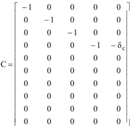
A, B and C represent, respectively, the following (10x10), (10x10) and (10x5) matrices:
− − − − − − = 1 0 0 0 0 0 0 0 0 0 0 1 0 0 0 0 0 0 0 0 0 0 1 0 0 0 0 0 0 0 0 0 0 0 0 0 0 1 0 0 0 0 0 0 0 0 0 0 0 1 0 0 0 0 0 0 0 0 1 0 0 1 0 0 0 0 0 0 δ δ 1 γ 0 0 0 0 0 µ γ ) µ (1 0 0 1 0 0 0 0 0 µ 0 0 β 0 0 0 0 0 0 β β π y r pa r pa π r r y A − − − − − − = 0 0 0 0 0 0 0 1 0 0 0 0 0 0 0 0 1 0 0 0 0 0 0 0 0 0 0 0 1 0 0 0 0 1 0 0 0 0 0 0 0 0 0 0 1 0 0 0 0 0 0 0 0 0 0 1 0 0 0 0 δ ρ 0 0 0 0 0 0 0 0 0 0 0 0 0 0 0 0 0 0 0 0 ) µ (1 0 0 0 0 0 0 α β 0 0 0 0 0 0 0 0 1 B pa y pa π
6 − − − − − = 0 0 0 0 0 0 0 0 0 0 0 0 0 0 0 0 0 0 0 0 0 0 0 0 0 0 0 0 0 0 δ 1 0 0 0 0 0 1 0 0 0 0 0 1 0 0 0 0 0 1 C c
Finally, the vector Zt consisting of a (5x1) vector containing the four disturbance terms and a
constant (ηt, τt, ξt, κt and 1). And the error vector is given by:
+ ⋅ = − − − − 0 ε ε ε ε 1 κ ξ τ η 1 0 0 0 0 0 0 0 0 0 0 0 ρ 0 0 0 0 0 ρ 0 0 0 0 0 ρ 1 κ ξ τ η t i t pa t s t d 1 t 1 t 1 t 1 t pa s d t t t t
Before proceeding with stochastic simulations we have to calibrate the parameters of our model and perform an analysis of its impulse-response functions. Such analysis will assess the reliability of the chosen system.
Regarding the parameters, the values presented in Table 1 correspond approximately to some
benchmark values previously employed in several papers5.
Table 1. Parameters (base model)6
βr 0,050 γr 0,200 βy 1 δc - 0,004 βpa 0,100 ρ 0,850 αy 0,200 δπ 0,500 µπ 0,500 δy 0,100 µpa 0,500 δpa 0,050
Finally, the standard deviations of random shocks (σd, σs, σi) are, respectively, 0,1, 0,03 and 0,1.
In relation to the random shock on asset prices, σpa, we could consider different values for
5
Among others: Fuhrer and Moore (1995), Gali and Gertler (1999), Rudebusch and Svensson (1999 and 2002), Gerlach and Schnabel (2000), Gali et al. (2001 and 2003) and Djoudad and Gauthier (2003). Where econometric evidence is not available, the parameters are calibrated to ensure plausible dynamic behaviour by the impulse responses.
6
In our model, δc = (1 - ρ) ⋅ [r + (1 - λπ) ⋅ π*], where ρ is the interest rate smoothing parameter, r is the
long term real interest rate, π* is the inflation target and λπ is the coefficient on inflation deviations from
target in a standard Taylor rule. Since δπ = (1 - ρ) ⋅ λπ, with δπ = 0,50 and ρ = 0,85, λπ is equal to 3,33.
Assuming that r and π* are both equal to 2 per cent, we obtain the value of -0,004 to δc (between 1997:1
7
equity and housing prices. Nevertheless, we will consider a joint value of 0,15. This configuration for the standard deviations, that is consistent with empirical findings, allows the volatility of asset prices to exceed the output gap volatility. On the contrary, inflation volatility is substantially lower, which is in accordance with the present price stability environment.
Finally, we consider those shocks orthogonal and that ρd = ρs = ρpa = 0,5.
3.2. Impulse-response functions
We solve numerically our linear rational expectations model since it’s not possible to find simple analytical solutions. For the system to have a unique stable solution it is necessary that the matrix A eingenvalues are inside the unit circle. We apply a modified version of the algorithm proposed by Klein (2000) and described in McCallum (1998 and 2001), using some
Matlab routines7. Such procedures allow the performance evaluation of different monetary
rules. Note that, by performance we mean the volatility generated by a particular rule, mainly in terms of inflation and output gap, with different specifications or values for particular parameters.
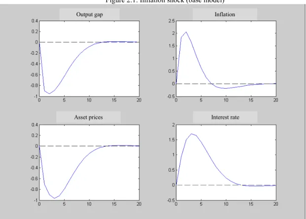
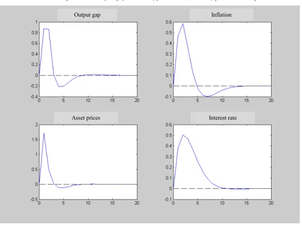
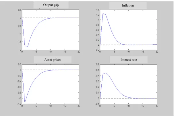
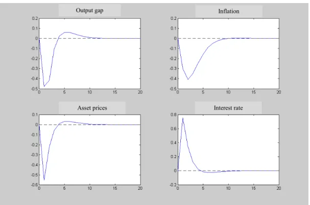
The resulting impulse-response functions, generated with the base model, are presented in Appendix 2. (Figures 2.1-2.3). Figure 2.1 presents the output gap, inflation, asset prices and interest rate responses to an inflation shock (negative supply shock). The output gap and asset prices fall whereas inflation and interest rate rise. With an output gap shock (demand shock), the initial response for the four variables is positive (Figure 2.2). With a monetary policy shock (Figure 2.3), we see that after a rise in interest rates, inflation, output and asset prices fall, a
result which is consistent with numerous studies based on autoregressive vectors (VAR)8. In
sum, the economic system that we are using seems well specified, since we established a monetary transmission mechanism that goes from the interest rate to the output gap, inflation and asset prices, without occurring a “price puzzle” in the inflation response or a negative effect of inflation on asset prices.
We can now compare those impulse-response functions with the results obtained with alternative calibrations of the base model. We will consider the following four alternative hypotheses:
(A) Stronger influence of asset prices on the output gap and absence of asset prices in
the policy rule. That is, βpa = 0,5 and δpa = 0 (Figures 2.4-2.6);
7
The main file is solvek.m, an algorithm to solve rational expectations models through the Schur generalized form that gives in many cases the same solution as the Blanchard and Khan (1980) stability criterion. We also use the impo.m and sim33p.m files to, respectively, generate impulse-response functions and perform the model’s stochastic simulations.
8
The application of VAR models to the European case was made, among others, by Gerlach and Smets (1995), Barran et al. (1997), Ramaswamy and Sloek (1997), Ehrmann (2000), Mojon and Peersman (2003), Peersman and Smets (2003) and Dedola and Lippi (2005).
8
(B) Absence of influence of asset prices on the output gap and strong importance of
them in the policy rule. That is, βpa = 0 and δpa = 0,2 (Figures 2.7-2.9);
(C) Absence of asset prices in both equations. That is, βpa = 0 and δpa = 0 (Figures
2.10-2.12);
(D) Stronger influence of asset prices on the output gap and strong importance of them
in the policy rule. That is, βpa = 0,5 and δpa = 0,2 (Figures 2.13-2.15).
Comparing Figures 2.1 to 2.3 with Figures 2.4 to 2.15, and considering the possibility of shocks on inflation, output gap and interest rates, we conclude that:
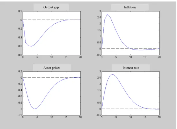
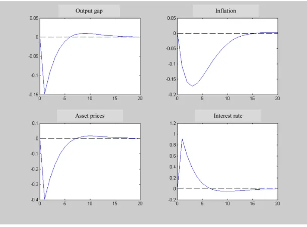
(1) The occurrence of an inflation shock, in the hypothesis of asset prices having a stronger impact on output gap albeit not being considered in the policy rule [hypothesis (A)], will provoke a stronger fall of the output gap and asset prices, being smaller the inflation response (Figure 2.4). Given that same type of shock, but if now asset prices don’t influence the output gap, albeit entering in the policy rule [hypothesis (B)], we observe similar responses to the base model, with the exception of a substantially stronger interest rate response, but with a greater time period to the return to the stationary state values (Figure 2.7). Considering the inexistence of an influence of asset prices on both output gap and interest rate [hypothesis (C)], we observe an extremely similar response to the previous one (Figure 2.10), which indicates that, with a weak influence of asset prices on the output gap, it will be difficult to accept their inclusion in a monetary policy rule. Finally, considering a significant presence of asset prices in the demand equation and in the policy rule [hypothesis (D)], we observe relatively stronger movements in the output gap and asset prices, which demand a lower interest rate response (Figure 2.13);
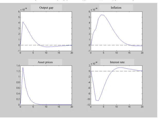
(2) Analysing now the effects of an output gap shock, we see that hypothesis (A) provokes a much higher effect on output gap and inflation, which generates a stronger interest rate response (Figure 2.5). With a demand shock, but with hypothesis (B), we observe an inverse response, albeit of lower magnitude, from the output gap and inflation (Figure 2.8). That generates some volatility on interest rates, since that variable initially diminishes, but thereafter increases to control asset prices evolution. So, imposing the need of this response becomes destabilizing. Comparing this situation with Figure 2.11, where hypothesis (C) is considered, we see that the withdrawal of asset prices from the rule would be desirable when asset prices don't influence the output gap. In that case, with the exception of asset prices, the responses have an extremely low magnitude. Figure 2.14 displays the results from hypothesis (D). With a strong effect from asset prices on the output gap and with monetary policy acting accordingly, when we put a relatively higher weight of that variable in the policy rule we observe stronger responses from all variables, namely, the interest rate;
9
(3) Finally, comparing the effects of an interest rate shock we see that, with hypothesis (A), where asset prices have a stronger impact on output gap but aren't considered in the policy rule (Figure 2.6), output gap and inflation have more pronounced responses, whereas with hypothesis (2), we see weaker responses for those two variables (Figure 2.9). When hypothesis (C) is considered, we obtain similar results (Figure 2.12). That is, we conclude that if asset prices don't influence output gap there seems to exist no advantage of an interest rate response to the deviations of that variable from a particular long run trend. Finally, considering hypothesis (D), whose results are displayed in Figure 2.15, we observe the existence of a stronger response from output gap and inflation, when compared with the base model. Yet, comparing Figure 2.6 with Figure 2.15, which has similar responses, we conclude that even if asset prices significantly influence the output gap that will not create substantial differences in the response pattern and respective volatilities of the relevant variables.
In conclusion, it seems to be desirable to withdraw asset prices from the monetary policy rule since – and given the results from the empirical literature pointing to non-significant effects of asset prices on demand – the failure to do so would provoke an higher instability of the different macroeconomic variables and the need for an higher number of periods for the variables to return to their baseline values, with the exception of asset prices, whose control should not be a concern for the monetary authorities. Furthermore, as we can see by analysing the different impulse-response functions, independently of the shocks occurring in the economy, in case asset prices decisively influence output gap, the fact that the monetary authority responds or not to the asset prices deviations becomes irrelevant in terms of the response pattern and volatility of the different considered endogenous variables.
In the following section, through the definition of a set of loss functions for the society, we will try to quantify the costs associated to the different strategies.
3.3. Alternative policy choices
We begin this section by showing some of the results from the different stochastic simulations performed. The stochastic simulations are made with the routine sim3p.m, departing from a basic specification and varying the parameters in the reaction function and/or some of the parameters from the other calibrated equations. Routine sim33p.m examines the stochastic properties of the model from the realization of Monte Carlo simulations. That is, departing from a set of randomly selected numbers, we design a finite sequence of innovations corresponding to 100 simulation periods as an iterating horizon, deriving the simulated series for all the exogenous and endogenous variables and allowing the computation of statistics as the standard deviation of each variable. This procedure is repeated several times and the results are stored, so
10
that we can resume the empirical distribution of those statistics presenting the average standard deviations.
The Figures appearing in Appendix 3 (Figures 3.1 to 3.9), present the volatility evolution (standard deviation) of four endogenous variables – inflation rate, output gap, asset prices deviations and interest rate – considering several deviations from the base model parameters. Figures 3.1 to 3.3 present the volatility evolution of the different variables, considering the base
model and as parameter δπ rises. As we can observe, as the concern with inflation in the policy
rule rises we attain a substantial reduction in that variable volatility, along with a not very significant rise in the volatility of the other variables. Comparing that situation with the
hypothesis of non including asset prices in the policy rule (δpa = 0), there are no visible effects
in the volatilities for the different variables, being otherwise slightly lower the values for the inflation rate standard deviation. In the different figures we have also an alternative hypothesis:
asset prices don't influence the output gap but appear in the reaction function (βpa = 0). Tough,
with the exception of the output gap, such situation would contribute to raise the volatilities for all the considered variables.
Finally, in the context of this base model, let's point to two aspects that are not graphically presented: in the first place, should parameter ρ presented a lower value, which would imply a lower concern from the monetary authority with interest rate smoothing, this variable would present a much higher volatility, albeit returning faster to its base value; in the second place, we could perform the model simulation with an exclusively backward or forward looking equation for price adjustments. In the first case, the return to the steady-state would be generally slower, with a lower inflation rate response. In the second case, the return would be faster, with shorter responses for inflation and output gap.
Figures 3.4 to 3.6 present the volatility evolution of the different variables as the parameter δy
rises, in comparison with the base model. As we raise the output gap weight in the reaction function we obtain a reduction in its volatility, though there's a significant rise in the inflation
volatility. Note also that the rise in δy contributes to a lower volatility in asset prices, not
affecting the interest rate volatility. Comparing this situation with the hypothesis of non including asset prices in the policy rule, we have a significant reduction in the volatility for the different variables, again with the exception of output gap. Finally, comparing with the alternative hypothesis of asset prices not influencing the output gap, albeit appearing in the reaction function, we conclude that such situation would not generate significant differences in relation to the base model.
Finally, Figures 3.7 to 3.9 present the volatility evolution for the different variables as the
parameter δpa rises, compared with the base model. As we raise the weight for the asset prices
11
in inflation and interest rate volatilities, along with a reduction in the output gap volatility. Comparing this situation with the alternative hypothesis that asset prices don’t influence the
output gap but appear in the reaction function, we see that as δpa rises, there's a rise in the
volatility for the considered variables, namely for inflation and interest rate, with the exceptions of asset prices and output gap. Finally, should asset prices exert a strong influence over the output gap, albeit the rise in the inflation volatility (with lower values compared with the base model), their inclusion in the policy rule could be justified because that would contribute to reduce the output gap volatility and even the volatility of asset prices.
So, the inclusion in the reaction function of a response to asset prices deviations contributes to a general increase in inflation and interest rate volatilities. On the other hand, the presence of asset prices deviations in the reaction function contributes to reduce the output gap volatility. Note that, the “optimal” policy choice is always dependent of the relevance or severity level given by the economy to the volatility displayed by the different variables.
Albeit we are not computing here an optimal policy rule, we can consider that the monetary authorities wish that its policy effects minimize the society losses in terms of welfare. We can consider the existence of a given loss function (L), whose value is determined by the volatility registered by the endogenous variables and assume that the society intends to keep that volatility low. Note, as also highlighted by Kontonikas and Ioannidis (2005) that it’s not common Central Bank practice to reveal loss functions or targets of this kind or the weights given to each variable.
In this case, the total loss can be computed as a linear combination of a set of standard deviations (s.d.):
L = a ⋅ (s.d.π) + b ⋅ (s.d.y) + c ⋅ (s.d.pa) + d ⋅ (s.d.i) (11)
being a, b, c and d the respective weights that the central bank attaches to the volatility in inflation, output gap, asset prices deviations and interest rates.
We are going to consider seven alternative sets of weights, which when applied to the base
model stochastic simulation results (and also to the base model with δy = 0 and/ or δpa = 0) and
to the four alternative specifications already considered in the previous section (respectively, βpa
= 0,5 and δpa = 0; βpa = 0 and δpa = 0,2; βpa = 0 and δpa = 0; βpa = 0,5 and δpa = 0,2), allow us to
12
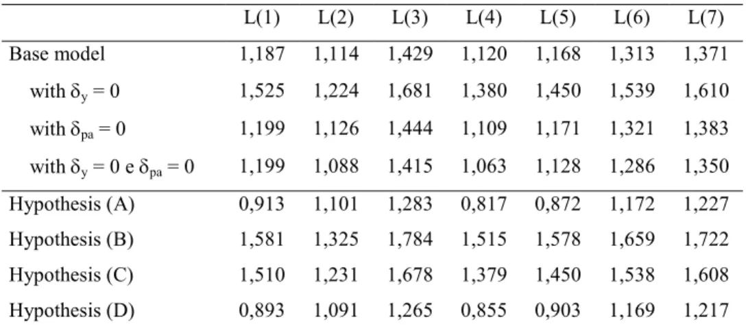
Table 2. Loss function values
L(1) L(2) L(3) L(4) L(5) L(6) L(7) Base model 1,187 1,114 1,429 1,120 1,168 1,313 1,371 with δy = 0 1,525 1,224 1,681 1,380 1,450 1,539 1,610 with δpa = 0 1,199 1,126 1,444 1,109 1,171 1,321 1,383 with δy = 0 e δpa = 0 1,199 1,088 1,415 1,063 1,128 1,286 1,350 Hypothesis (A) 0,913 1,101 1,283 0,817 0,872 1,172 1,227 Hypothesis (B) 1,581 1,325 1,784 1,515 1,578 1,659 1,722 Hypothesis (C) 1,510 1,231 1,678 1,379 1,450 1,538 1,608 Hypothesis (D) 0,893 1,091 1,265 0,855 0,903 1,169 1,217
Note: L(i) = (a; b; c; d): L(1) = (1; 1; 1; 1); L(2) = (2; 2; 0; 0); L(3) = (2; 2; 0,5; 0,5); L(4) = (2; 1; 0; 0,5); L(5) = (2; 1; 0,25; 0,5); L(6) = (2; 2; 0; 0,5); L(7) = (2; 2; 0,25; 0,5).
Notice that this analysis is dependent upon the relative significance given to the different weights. The fact that L(1) through L(7) give always a greater relative significance to inflation and output gap only reflects the evidence that those two variables are generally the most important in any loss function.
As we can observe, and comparing with the base model, when asset prices have a strong effect on output gap, it will be somehow desirable that monetary policy responds counter-cyclically to its evolution [in general, when comparing hypothesis (A) with hypothesis (D), there is a slight fall in the loss values]. Anyway, the fall in the loss function values are small, so that the gains from that shouldn't offset the potential costs arising from an explicit monitoring of asset prices by the monetary authority (namely, the occurrence of moral hazard incentives). Nevertheless, faced with a non-significant or null impact of asset prices on demand, the inclusion of those in the monetary policy rule would be extremely destabilising, generating a significant rise in the values for the loss function. That is, if asset prices don't influence the output gap it would be very difficult to justify some kind of response to them by the monetary authority [we can also compare the results between hypothesis (B) and (C)]. Also, this kind of result is present in some papers [e.g., Batini and Nelson (2000)], which go against the results from Cecchetti et al. (2000), who evidenced that a small interest rate reaction to asset price deviations gave some contribution to reduce the macroeconomic volatility. The values presented in the second line of Table 2 indicate that, when compared to the base model, the absence of a monetary authority response to the output gap generates slightly higher values for the different loss functions. So, in spite the higher weight given to inflation in the policy rule, the monetary authority should keep
some concern with the output gap behaviour, adopting a flexible inflation targeting regime9. The
values presented in the third and fourth lines of Table 2 show that, independently of the
9
Other authors [e.g., Bernanke and Gertler (2001) and Kontonikas and Ioannidis (2003)], also conclude that the output gap has an independent role in the reaction function.
13
influence of asset prices on the output gap, whether the monetary authority is sensitive or not to them generates almost identical values for the loss functions when compared with the base model. Finally, in the case where the authorities in its loss function give a higher importance to asset prices deviations, its “optimal” monetary policy will react to asset prices, trying to reduce
their volatility10. Albeit here we are not presenting those results, we could observe what would
happen to the different loss function values if the monetary policy weren’t sensible to the output gap, in spite of considering asset prices deviations in its reaction function. In that case, when asset prices have some influence over the output gap, it would be advisable to include them in the reaction function, yet an excessive weight in that function would contribute to a higher volatility for the different variables. In the case where asset prices exert a minor or null influence over the output gap, it would be advisable in terms of society welfare that the monetary authority abstained to react to asset prices deviations.
The behaviour of the loss function values can also be analysed in connection with the importance given to inflation, output gap or asset prices deviations in the policy rule. Figures 3.10 to 3.15, presented in Appendix 3, display the evolution of the different loss function values
when parameters δπ (Figures 3.10 and 3.11), δy (Figures 3.12 and 3.13) and δpa (Figures 3.14
and 3.15) change.
With the exception of Figures 3.10 and 3.11, and as parameters δy and δpa rise, we see a
generalized rising in the values for the different loss functions considered. Such behaviour means that if it is desirable a lower volatility for the relevant endogenous variables the policy rule should assign a small importance to output gap and asset prices movements (between the two extreme cases it is generated a rise of 0,2-0,3 points in the values for the loss function). Yet,
when we consider a rise in the parameter associated to inflation in the policy rule (δπ) we see an
almost generalized fall in the values for the different loss functions (Figures 3.10 and 3.11). So, we conclude that, in order to maximize welfare the policy rule should give a substantially larger attention to inflation, independently of the weak or even moderated effects of asset prices deviations on the output gap. The fact that this general conclusion gives us some insights about the conduct of monetary policy is explored in the next section.
10
In a recent publication, the ECB states that (ECB, 2005, p. 58): “A policy of ‘leaning against the wind’ would appear more attractive the higher the costs that the central bank ascribes to large, fundamentally unjustified swings in the valuation of assets (…)”.
14
4. Conclusion
The new-keynesian models are broadly used to examine issues of monetary policy and dynamic effects of shocks. The strength of those models emanate from their microeconomic foundations which, together with their simplicity, leads to behaviour and propagation mechanisms that are easily understood.
In a synthetic way, we can resume the main conclusions from the calibration and stochastic simulation of our model:
(1) Impulse-response functions reveal an apparently well specified model, being established a transmission mechanism that goes from interest rates to inflation and asset prices, consistent with the stylized facts of the monetary policy dynamic effects;
(2) By observing the impulse-response functions we conclude that it wouldn’t be desirable to include asset prices in the monetary policy rule, since that would generate a higher instability for the different macroeconomic variables and the need for a higher number of periods for the variables return to their steady-state values;
(3) The monetary policy rule should contain a relatively strong weight for inflation yet, since the output gap is useful to predict future inflation, it should leave a small independent role for that variable;
(4) The inclusion of a reaction to asset prices deviations in the monetary policy rule would only be justifiable in the context of a strong sensibility from the part of the output gap and, even in that case, the gains in terms of welfare would be small, in a way that shouldn’t offset the costs attached to an explicit tracking of asset prices behaviour by the monetary authority.
So, our results seem to suggest that asset prices aren’t a fundamental variable for monetary policy, in spite of their potential to represent an important aspect in the formulation of that policy, as happens with the European Central Bank (ECB). In other words, our results are consistent with the view that, tough committed with the control of inflation, and in a lesser way of output gap, central banks could act in response to asset prices movements when there’s the need to avoid a sharp correction in the markets, which could have destabilising effects over the economy. Thus, the benign neglect perspective prevails and apparently the ECB fits in this pattern, as evidenced by its moves in 2007 to calm down the effects of the subprime crisis over the financial markets.
15
References
Amato, J. and Laubach, T. (2004), “Implications of Habit Formation for Optimal Monetary Policy”, Journal of Monetary Economics, 51, 305-325.
Aoki, K., Proudman, J. and Vlieghe, G. (2004), “House Prices, Consumption, and Monetary Policy: a financial accelerator approach”, Journal of Financial Intermediation, 13 (4), October, 414-435.
Barran, F., Coudert, V. and Mojon, B. (1997), “The Transmission of Monetary Policy in the European Countries”, In S. Collignon (Ed.), European Monetary Policy. Pinter Press.
Batini, N. and Nelson, E. (2000), “When the Bubble Bursts: monetary policy and foreign exchange market behaviour”, Working Paper, Bank of England.
Bernanke, B. and Gertler, M. (1999), “Monetary Policy and Asset Price Volatility”, Economic Review, Federal Reserve Bank of Kansas City, 84 (4), 17-51.
Bernanke, B. and Gertler, M. (2001), “Should Central Banks Respond to Movements in Asset Prices?”, American Economic Review, 91 (2), May, 253-257.
Blanchard, O. and Khan, C. (1980), “The Solution of Linear Difference Models under Rational Expectations”, Econometrica, 48 (5), 1305-1311.
Cecchetti, S., Genberg, H., Lipsky, J. and Wadhwani, S. (2000a), “Asset Prices and Central Bank Policy”, Geneva Reports on the World Economy, 2, London: International Center for Monetary and Banking Studies and CEPR.
Cecchetti, S., Chu, R. and Steindel, C. (2000b), “The Unreliability of Inflation Indications”, In Current Issues in Economics and Finance, Federal Reserve Bank of New York, 6 (4).
Dedola, L. and Lippi, F. (2005), “The Monetary Transmission Mechanism: evidence from the industries of five OECD countries”, European Economic Review, 49 (6), August, 1543-1569.
Durré, A. (2001), “Would it be Optimal for Central Banks to Include Asset Prices in their Loss Function?”, Working Paper – Institut de Recherches Économiques et Sociales, Université Catholique de Louvain, June.
ECB (2005), Montlhy Bulletin, April, European Central Bank, Frankfurt.
Ehrmann, M. (2000), “Comparing Monetary Policy Transmission across European Countries”, Weltwirtschaftliches Archiv, 136 (1), 58-83.
Frenkel, J. and Mussa, M. (1985), “Asset Markets, Exchange Rates and the Balance of Payments”, In R. Jones and P. Kenen (Eds.), Handbook of International Economics, 2, New York / Amsterdam: North Holland.
Fuhrer, J. and Moore, G. (1995), “Inflation Persistence”, Quarterly Journal of Economics, 110 (1), 127-159.
Gali, J. and Gertler, M. (1999), “Inflation Dynamics: a structural econometric analysis”, Journal of Monetary Economics, 44 (2), October, 195-222.
Gali, J., Gertler, M. and López-Salido, D. (2001), “European Inflation Dynamics”, European Economic Review, 45 (7), June, 1237-1270.
Gali, J., Gertler, M. and López-Salido, D. (2003), “Robustness of the Estimates of the Hybrid New-Keynesian Phillips Curve”, Working Paper, New York University.
Gerlach, S. and Schnabel, G. (2000), “The Taylor Rule and Interest Rates in the EMU Area”, Economic Letters, 67, 165-171.
16
Gerlach, S. and Smets, F. (1995), “The Monetary Transmission Mechanism: evidence from the G-7 countries”, Working Paper, Bank for International Settlements, 26, April.
Goodhart, C. and Hofmann, B. (2001), “Asset Prices, Financial Conditions and the Transmission of Monetary Policy”, paper presented at the conference Asset Prices, Exchange Rate, and Monetary Policy, Stanford University, March.
Hu, Z. (2003a), “Financial Asset Prices and US Monetary Policy”, Working Paper, Boston College. Hu, Z. (2003b), “Role of Housing Prices in the Monetary Business Cycle”, Working Paper, Boston College.
Klein, P. (2000), “Using the Generalized Schur Form to Solve a Multivariate Linear Rational Expectations Model”, Journal of Economic Dynamics and Control, 24, 1405-1423.
Kontonikas, A. and Ioannidis, C. (2005), “Should Monetary Policy Respond to Asset Price Misalignments?”, Economic Modelling, 22 (6), December, 1105-1121.
Ludvigson, S. and Steindel, C. (1999), “How Important is the Stock Market Effect on Consumption?”, Economic Policy Review, Federal Reserve Bank of New York, 5 (2), July, 29-51.
Ludvigson, S., Steindel, C. and Lettau, M. (2002), “Monetary Policy Transmission Through the Consumption Wealth Channel”, Economic Policy Review, Federal Reserve Bank of New York, May, 117-133.
McCallum, B. (1998), “Solutions to Linear Rational Expectations Models: a compact exposition”. Economic Letters, 61, 143-147.
McCallum, B. (2001), “Software for RE Analysis”, mimeo, reviewed at 17th February 2004.
McCallum, B. and Nelson, E. (1999), “An Optimizing IS-LM Specification for Monetary Policy and Business Cycle Analysis”, Journal of Money, Credit, and Banking, 31 (1), 296-316.
Mojon, B. and Peersman, G. (2001), “A VAR Description of the Effects of Monetary Policy in the Individual Countries of the Euro Area”, in Angeloni et al. (Eds.), Monetary Policy Transmission in the Euro Area, Cambridge University Press, 2003, chp. 1, 56-74.
Nisticò, S. (2005), “Monetary Policy and Stock Prices in a DSGE Framework”, Working Document, Dipartimento di Scienze Economiche e Aziendali – Universitá Luiss Guido Carli, 28, April.
Ortalo-Magne, F. and Rady, S. (1998), “Housing Market Fluctuations in a Life-Cycle Economy with Credit Constraints”, GSB Research Paper, Stanford University, 1501.
Pacheco, L. (2004), “Asset Prices and Monetary Policy in the Euro Area: a tentative model”, In Yiannis Stivachtis (Ed.), Current Issues in European Integration, 461-492, ATINER, Athens.
Peersman, G. and Smets, F. (2003), “The Monetary Transmission Mechanism in the euro area: more evidence from VAR analysis”, in Angeloni et al. (Eds.), Monetary Policy Transmission in the Euro Area, Cambridge University Press, 2003, chp. 2, 36-55.
Ramaswamy, R. and Sloek, T. (1997), “The Real Effects of Monetary Policy in the European Union: what are the differences?”, International Monetary Fund, Working Paper, 97, December.
Rudebusch, G. and Svensson, L. (1999), “Policy Rules for Inflation Targeting”, in J.B. Taylor (ed.), Monetary Policy Rules, 203-246, Chicago: University of Chicago Press.
Rudebusch, G. and Svensson, L. (2002), “Eurosystem Monetary Targeting: lessons from US data”, European Economic Review, 46 (3), 417-442.
17
Svensson, L. (1997), “Inflation Forecast Targeting: implementing and monitoring inflation targets”, European Economic Review, 41 (6), 1111-1146.
Svensson, L. (1999), “Inflation Targeting: some extensions”, Scandinavian Journal of Economics, 101 (3), 337-361.
18
APPE"DIX1
Considering equities as the relevant asset, the approach taken here to obtain the asset prices equation starts with the definition of the return obtained in the equity market:
Rt+1 ≡ S 1 D S t 1 t 1 t+ + + − (1.1)
where Rt+1 represents the one-period return from equities (from t to t+1), St represents the equity
price at t and Dt+1 represents the next period dividend.
With a first-order Taylor expansion around the steady-state equation (1.1) becomes:
1 t _ _ t _ _ _ 1 t 1 t _ d S D pa S D S pa r ι + ≈ + − + + + (1.2) where: ιt+1 = Rt+1 + 1; r log(ι ) log(ι); _ 1 t 1 t+ = + − pa log(S ) log(S); _ 1 t 1 t+ = + − pa log(S) log(S); _ t t = − _ _ _ _ 1 t 1
t log(D ) log(D) and ι ,S andD
d+ = + − are steady-state values.
Multiplying both sides of equation (1.2) by _ _
_
D S
S
+ and rearranging, we obtain:
pat ≈ µpa ⋅ pat+1 + (1-µpa) ⋅ dt+1 - γr ⋅ rt+1 (1.3) where _ _ _ _ r _ _ _ pa D S S ι γ and , D S S µ + = + = .
Following Durré (2001), the real dividend at t+1 is proportional to the expected output level in period
t+1, so that dt+1 ≈ Etyt+1. In the same way, pat+1 is unknown, being given by Etpat+1.An arbitrage
condition helps to assume that the expected real interest rate, rt+1, is equal to it - Etπt+1, and υt is a
time-varying risk premium. So, we obtain the following equation:
rt+1 = it - Etπt+1 + υt (1.4)
Combining equations (1.3) and (1.4), we obtain the following dynamic equation for asset prices:
pat = µpa⋅Etpat+1 - γr⋅(it - Etπt+1) + (1-µpa)⋅Etyt+1 + ξt (1.5)
where ξt = - γr⋅υt, can be interpreted as an equity premium shock of the type discussed in Cecchetti et
al. (2000b). Nothe that this forward looking equation for asset prices constitutes a version of the Frenkel and Mussa (1985) asset prices equation, where asset prices deviate from their fundamental
level. Finally, the disturbance term ξt encompasses non-fundamental factors
11
. There are several
possible interpretations for pat (e.g., housing prices, equity prices or the value of a portfolio
containing both), tough for now we have treated pat simply as based in an equity market index.
11
Kontonikas and Ioannidis (2005), in the context of a similar model, consider a backward looking influence over asset prices. For the derivation of the equity prices dynamic equation, in the context of a DSGE model, see Nisticò (2005).
19
We don’t interpret shocks over asset prices, ξt, as speculative bubbles, referring instead to exogenous
risk premium stochastic fluctuations, namely motivated by investors risk aversion. Even though Smets (1997) and Durré (2001) consider the shock over equity prices as white noise, we also assume that shocks follow univariated AR(1) processes:
ξt = ρpa ⋅ ξt-1 + ε
pa
t (1.6)
20
APPE"DIX 2: Impulse response functions Figure 2.1: Inflation shock (base model)
Figure 2.2: Output gap shock (base model) Output gap Output gap Asset prices Asset prices Inflation Inflation Interest rate Interest rate
21
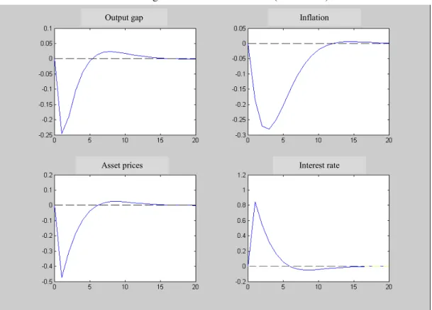
Figure 2.3: Interest rate shock (base model)
Figure 2.4: Inflation shock: hypothesis (A), with βpa = 0,5 and δpa = 0
Output gap Output gap Asset prices Asset prices Inflation Inflation Interest rate Interest rate
22
Figure 2.5: Output gap shock: hypothesis (A), with βpa = 0,5 and δpa = 0
Figure 2.6: Interest rate shock: hypothesis (A), with βpa = 0,5 and δpa = 0
Output gap Output gap Asset prices Asset prices Inflation Inflation Interest rate Interest rate
23
Figure 2.7: Inflation shock: hypothesis (B), with βpa = 0 and δpa = 0,2
Figure 2.8: Output gap shock: hypothesis (B), with βpa = 0 and δpa = 0,2
Output gap Output gap Asset prices Asset prices Inflation Inflation Interest rate Interest rate
24
Figure 2.9: Interest rate shock: hypothesis (B), with βpa = 0 and δpa = 0,2
Figure 2.10: Inflation shock: hypothesis (C), with βpa = 0 and δpa = 0
Output gap Output gap Asset prices Asset prices Inflation Inflation Interest rate Interest rate
25
Figure 2.11: Output gap shock: hypothesis (C), with βpa = 0 and δpa = 0
Figure 2.12: Interest rate shock: hypothesis (C), with βpa = 0 and δpa = 0
Output gap Output gap Asset prices Asset prices Inflation Inflation Interest rate Interest rate
26
Figure 2.13: Inflation shock: hypothesis (D), with βpa = 0,5 and δpa = 0,2
Figure 2.14: Output gap shock: hypothesis (D), with βpa = 0,5 and δpa = 0,2
Output gap Output gap Asset prices Asset prices Inflation Inflation Interest rate Interest rate
27
Figure 2.15: Interest rate shock: hypothesis (D), with βpa = 0,5 and δpa = 0,2
Output gap
Asset prices
Inflation
28
APPE"DIX 3: Volatility evolution in the endogenous variables (standard deviations: s.d.)
Figure 3.1: inflation s.d. vs. output gap s.d.
Figure 3.2: inflation s.d. vs. interest rate s.d.
29
Figure 3.4: inflation s.d. vs. output gap s.d.
Figure 3.5: inflation s.d. vs. interest rate s.d.
30
Figure 3.7: inflation s.d. vs. output gap s.d.
Figure 3.8: inflation s.d. vs. interest rate s.d.
31
Figures 3.10 and 3.11: loss functions values evolution (δπ increasing)
Figures 3.12 and 3.13: loss functions values evolution (δy increasing)
0,00 0,20 0,40 0,60 0,80 1,00 1,20 1,40 1,60 1,80 2,00 0 ,2 0 ,2 5 0 ,3 0 ,3 5 0 ,4 0 ,4 5 0 ,5 0 ,5 5 0 ,6 0 ,6 5 0 ,7 0 ,7 5 0 ,8 0 ,8 5 0 ,9 0 ,9 5 1 delta(inf) L(1) L(2) L(3) 0,00 0,20 0,40 0,60 0,80 1,00 1,20 1,40 1,60 1,80 2,00 0 ,2 0 ,2 5 0 ,3 0 ,3 5 0 ,4 0 ,4 5 0 ,5 0 ,5 5 0 ,6 0 ,6 5 0 ,7 0 ,7 5 0 ,8 0 ,8 5 0 ,9 0 ,9 5 1 delta(inf) L(4) L(5) L(6) L(7) 0,00 0,20 0,40 0,60 0,80 1,00 1,20 1,40 1,60 1,80 2,00 0 0 ,0 5 0 ,1 0 ,1 5 0 ,2 0 ,2 5 0 ,3 0 ,3 5 0 ,4 0 ,4 5 0 ,5 0 ,5 5 0 ,6 0 ,6 5 0 ,7 0 ,7 5 0 ,8 0 ,8 5 0 ,9 0 ,9 5 1 delta(y) L(1) L(2) L(3)
32
Figures 3.14 and 3.15: loss functions values evolution (δpa increasing)
0,00 0,20 0,40 0,60 0,80 1,00 1,20 1,40 1,60 1,80 2,00 0 0 ,0 5 0 ,1 0 ,1 5 0 ,2 0 ,2 5 0 ,3 0 ,3 5 0 ,4 0 ,4 5 0 ,5 0 ,5 5 0 ,6 0 ,6 5 0 ,7 0 ,7 5 0 ,8 0 ,8 5 0 ,9 0 ,9 5 1 delta(y) L(4) L(5) L(6) L(7) 0,00 0,20 0,40 0,60 0,80 1,00 1,20 1,40 1,60 1,80 2,00 0 0 ,1 0,2 0,3 0,4 0,5 0,6 0,7 0,8 0,9 1 delta(pa) L(1) L(2) L(3) 0,00 0,20 0,40 0,60 0,80 1,00 1,20 1,40 1,60 1,80 2,00 0 0 ,1 0,2 0,3 0,4 0,5 0,6 0,7 0,8 0,9 1 delta(pa) L(4) L(5) L(6) L(7)
33 CIGE – Centro de Investigação em Gestão e Economia
Universidade Portucalense – Infante D. Henrique
Rua Dr. António Bernardino de Almeida, 541/619 4200-072 PORTO PORTUGAL http://www.upt.pt cige@uportu.pt ISSN 1646-8953