Spatial and spatio-temporal point patterns on linear
networks
Dissertation submitted by Mohammad Mehdi Moradi to apply for the joint doctorate degree from the Universitat Jaume I, Universidade Nova de Lisboa and
Universit ¨at M ¨unster.
European Joint Doctorate Marie Sklodowska-Curie in
Geoinformatics
Doctoral School from Universitat Jaume I
Mohammad Mehdi Moradi
Supervisors:
Jorge Mateu Ana Cristina Costa Edzer Pebesma
(Universitat Jaume I) (Universidade Nova de Lisboa) (Universit ¨at M ¨unster)
This dissertation is funded by the European Commission within the Marie Skłodowska-Curie Actions (ITN-EJD). Grant Agreement num. 642332 - GEO-C - H2020-MSCA-ITN-2014.
i
iii
Acknowledgments
First of all I would like to express my sincere gratitude to my supervisor Jorge Mateu for his continuous support, patience, motivation, and immense knowledge. Besides, I would like to thank my co-supervisor Edzer Pebesma who provided me with the opportunity of visiting his research group during my external semester and also for his insightful comments, encouragement and being always in my disposal. I also thank my co-supervisor Ana Cristina Costa for her thoughtful comments and encouragement.
My sincere thanks also goes to Adrian Baddely, Ottmar Cronie and Ege Rubak who provided me the opportunity to visit their research group and collaborate with them in several projects. I am also grateful to Gopalan Nair, Tilman M. Davies, Suman Rakshit and Raphael Lachieze-Rey that I had the pleasure to work with them during my phd.
I take this opportunity to thank the members of GEOTEC for their help and encouragement, especially Carlos Granel and Sergi Trilles. Special thanks go to my friends Fernando Benitez, Carolina Jimenez, Diego Pajarito, Manuel Portela and Khoi Manh for their support, encouragement and helps.
I would also thank Janine Illian and Rasmus Waagepetersen for their helpful comments and suggestions.
Last but not least, I would like to give further thanks to my family for their continued support and encouragement throughout my studies and life.
v
Resumen
Los datos con componente espacial suelen formarse con diferentes tipos de geometr´ıas, como pueden ser lineales, poligonales o puntuales, entre otras. Estas ´ultimas, las puntuales, est ´an formadas por pares de coordenadas, las cuales se consideran patrones y los puntos son llamados eventos. Estos pueden estar distribuidos de forma regular o irregular dentro de un mismo espacio. Esta distribuci ´on puede darse en contextos muy variados, como puede ser en las ciencias geoespaciales, ecolog´ıa, astronom´ıa, econometr´ıa, criminolog´ıa, entre otros. Por ejemplo, los puntos pueden representar desde ´arboles dentro de un bosque, accidentes de tr ´afico o cr´ımenes en una ciudad. En Møller and Waagepetersen (2003); Baddeley and Turner (2005); Illian et al. (2008); Gelfand et al. (2010); Okabe and Sugihara (2012); Diggle (2003); Baddeley et al. (2015) se pueden encontrar diferentes ejemplos de este tipo de datos. Muchos de los patrones observados tambi ´en pueden incluir una componente temporal, y son llamados patrones espacio-temporales. En ocasiones, la ubicaci ´on de los objetos se registra de forma regular o irregular a trav ´es del tiempo. En este caso, cada objeto tiene un conjunto de puntos consecutivos que definen una trayectoria. Con lo que se obtiene, no solo unos patrones de puntos, sino un patr ´on de las trayectorias, como puede ser el movimiento de taxis, animales, humanos, etc. La actual tesis, se centra principalmente en los patrones puntuales espaciales y espacio-temporales que suceden en una red lineal, como pueden ser los accidentes en las calles de una ciudad. Finalmente, tambi ´en se incluyen el an ´alisis de las trayectorias. La tesis se estructura de la siguiente manera:
En primer lugar, se presenta un cap´ıtulo introductorio (Cap´ıtulo 1) en el que se muestra un breve resumen de la teor´ıa de los procesos puntuales espaciales en R2, redes lineales y trayectorias. De ellos, se presentan conceptos b ´asicos a nivel
vi
abstracto e introduciendo de ellos algunas caracter´ısticas importantes. Tambi ´en, se definen te ´oricamente algunos modelos cl ´asicos de procesos puntuales. Se presentan los estimadores de intensidad, summary-statistics y relative risk.
El Cap´ıtulo 2 tiene como objetivo revisar y proponer algunos estimadores de intensidad basados en kernel para patrones de puntos espaciales en redes lineales, junto con el estudio de sus propiedades. La estimaci ´on de la intensidad de los patrones de puntos en redes lineales, como es el caso de una red de carreteras, parece ser una tarea complicada (Rakshit et al., 2018). Varias t ´ecnicas publicadas en la literatura en los contextos de geograf´ıa e inform ´atica, han resultado ser err ´oneas carreteras, parece ser una tarea complicada (Rakshit et al., 2018). Las t ´ecnicas existentes tambi ´en son computacionalmente costosas, especialmente cuando se analizan gran cantidad de datos, es decir, conjuntos de datos con una alta concentraci ´on de puntos y/o una gran red (Rakshit et al., 2018). Existen trabajos en la literatura que proponen estimadores de intensidad Borruso (2003, 2005, 2008); Xie and Yan (2008); Okabe et al. (2009); McSwiggan et al. (2017). Adem ´as, en este mismo cap´ıtulo se revisan algunos de los estimadores de intensidad actuales y se proponen dos nuevos estimadores, con el objetivo de mejorar los actuales, tanto estad´ısticamente como computacionalmente. En primer lugar, se presenta un estimador de intensidad basado en kernel, el cual aplica una correcci ´on de borde y revisa sus propiedades estad´ısticas (Moradi et al., 2017) tales como unbiasedness, mass conservation y variance. Mediante una simulaci ´on, se prueba su rendimiento estad´ıstico y se compara con el de Okabe et al. (2009); Okabe and Sugihara (2012). En segundo lugar, se propone un m ´etodo computacionalmente eficiente y con principios estad´ısticos de 2D convolution (Rakshit et al., 2018). Para ello se utiliza la transformada r ´apida de Fourier, la cual trabaja de forma eficiente incluso en redes grandes y para grandes bandwidth, y es robusta frente a posibles errores en la geometr´ıa de la red. Tambi ´en se discute el sesgo, variance, asymptotics, selecci ´on del bandwidth, estimaci ´on de variance, estimaci ´on de relative risk y adaptive smoothing. Adem ´as, se realiza un an ´alisis de su rendimiento y se compara con el de McSwiggan et al. (2017), tanto estad´ısticamente como computacionalmente. A lo largo del mismo cap´ıtulo, y utilizando los m ´etodos propuestos, tambi ´en se analizan varios conjuntos de datos reales como datos del crimen de Castell ´on, (Espa ˜na) y Chicago (EEUU) y los accidentes de tr ´afico de Medell´ın (Colombia) y Western Australia (Australia).
vii El Cap´ıtulo 3 propone una nueva t ´ecnica para proporcionar un estimador de intensidad adaptativo para procesos de puntos espaciales independientemente del state space (Moradi et al., 2018a). La t ´ecnica es introducida y aplicada a los estimadores de intensidad de Voronoi. Adem ´as, se revisan sus propiedades estad´ısticas y se estudia su comportamiento a trav ´es de diferentes simulaciones. Los estimadores de intensidad de Voronoi son adaptativos y no necesitan definir previamente par ´ametros; en ellos la estimaci ´on de intensidad est ´a condicionada por el tama ˜no rec´ıproco de la celda de Voronoi que contiene esa ubicaci ´on. Su principal inconveniente, se debe a que tiende a suavizar los datos en regiones donde la densidad puntual del patr ´on de punto observado es alta, siendo demasi-ado suave en regiones donde la densidad de puntos es baja. Para remediar este problema, es decir, para encontrar un t ´ermino medio entre el suavizado excesivo y el subestimado, se propone una t ´ecnica de suavizado adicional para estimadores de intensidad Voronoi para procesos puntuales en espacios m ´etricos arbitrarios, que se basa en aplicar repetidamente raleos independientes del proceso puntual (Moradi et al., 2018a). Se muestra que la t ´ecnica de remuestreo suavizado mejora la estimaci ´on de manera significativa. Adem ´as, se estudia las propiedades es-tad´ısticas, como la imparcialidad y la variance, y se propone una regla del pulgar y un enfoque de validaci ´on cruzada basada en datos para elegir la cantidad de diluci ´on/suavizado que se aplicar ´a. Tambi ´en se aplica a dos conjuntos de datos reales, en los accidentes de tr ´afico en un ´area de Houston (EEUU) (Patr ´on de punto de red lineal) y Finish pines que consiste en la ubicaci ´on de ´arboles en un bosque finland ´es (patr ´on de puntos de dos dimensiones).
El Cap´ıtulo 4 se centra en los procesos puntuales espacio-temporales en redes lineales. En algunos trabajos, solo se considera el dominio espacial y se analizan los patrones de puntos independientemente del tiempo, mientras que ellos est ´an ocurriendo inherentemente de forma conjunta en el espacio y el tiempo. Sin embargo, puede haber preguntas que el an ´alisis espacial no puede responder (Diggle, 2003). Para ello, se presentan varias caracter´ısticas de patrones de puntos espacio-temporales cuando las ubicaciones espaciales est ´an restringidas a una red lineal (Moradi et al., 2018b). Se propone un estimador de intensidad basado en kernel para resaltar la concentraci ´on alta/baja de eventos dentro de la red y el tiempo, ya sea de forma conjunta o por separado. Tambi ´en se utilizan caracter´ısticas de segundo orden de patrones de puntos espacio-temporales en redes lineales, como la funci ´on K-function y la funci ´on de correlaci ´on de pares
viii
para analizar el tipo de interacci ´on entre los puntos (Moradi et al., 2018b). Los cuales son independientes de la geometr´ıa de la red y tienen valores conocidos para los procesos de puntos de Poisson. Por lo que, se pueden usar para medir la desviaci ´on de Poisson y tambi ´en para la selecci ´on del modelo. Finalmente, tambi ´en se han utilizado diferentes conjuntos de datos reales, como por ejemplo los accidentes de tr ´afico en una ´area de Houston (EEUU), en una ´area de Medell´ın (Colombia) y una ´area de Eastbourne (Reino Unido).
El Cap´ıtulo 5 presenta se centra en las trayectorias. En el cual se proponen varias clases, m ´etodos y metodolog´ıas estad´ısticas, provenientes del paquete
trajectories de R para analizar conjuntos de datos en movimiento (Moradi et al.,
2018c). Hay que tener en consideraci ´on que el paquetetrajectories ampl´ıa a ´un
m ´as las capacidades del paquetespacetime (Pebesma, 2012). El R paquete
trajectories proporciona c ´odigos/funciones para manejar, simular y analizar
es-tad´ısticamente datos de movimiento independientemente del dominio y convertir un patr ´on de trayectoria en una lista de patrones de puntos basados en timestamps regulares. Para comprender el comportamiento de los objetos en movimiento, se propone un m ´etodo de estimaci ´on de la intensidad (para resaltar las calles y caminos m ´as visitadas), se realiza un an ´alisis de distancia, tambi ´en se presenta un suavizado de movimientos y se calcula el ´area de variabilidad de las carac-ter´ısticas de segundo orden (para ver los cambios del tipo de interacci ´on entre objetos a trav ´es del tiempo). Con el fin de comparar la intensidad estimada (ob-servada) con la intensidad esperada, se introducen los chimaps, que resaltan las
´areas con intensidad estimada m ´as alta/m ´as baja que la esperada. Tambi ´en se utilizan datos reales, en este caso de taxis en movimiento de Beijing (China).
Palabras clave: Estimador adaptativo, Intensidad, Kernel, Procesos puntuales,
ix
Abstract
The last decade witnessed an extraordinary increase in interest in the analysis of network related data and trajectories. This pervasive interest is partly caused by a strongly expanded availability of such datasets. In the spatial statistics field, there are numerous real examples such as the locations of traffic accidents and geo-coded locations of crimes in the streets of cities that need to restrict the support of the underlying process over such linear networks to set and define a more realistic scenario. Examples of trajectories are the path taken by moving objects such as taxis, human beings, animals, etc.
Intensity estimation on a network of lines, such as a road network, seems to be a surprisingly complicated task. Several techniques published in the literat-ure, in geography and computer science, have turned out to be erroneous. We propose several adaptive and non-adaptive intensity estimators, based on kernel smoothing and Voronoi tessellation. Theoretical properties such as bias, variance, asymptotics, bandwidth selection, variance estimation, relative risk estimation, and adaptive smoothing are discussed. Moreover, their statistical performance is studied through simulation studies and is compared with existing methods.
Adding the temporal component, we also consider spatio-temporal point pat-terns with spatial locations restricted to a linear network. We present a non-parametric kernel-based intensity estimator and develop second-order character-istics of spatio-temporal point processes on linear networks such as K-function and pair correlation function to analyse the type of interaction between points.
In terms of trajectories, we introduce the R packagetrajectories that contains
different classes and methods to handle, summarise and analyse trajectory data. Simulation and model fitting, intensity estimation, distance analysis, movement smoothing, Chi maps and second-order summary statistics are discussed.
x
Moreover, we analyse different real datasets such as a crime data from Chicago (US), anti-social behaviour in Castell ´on (Spain), traffic accidents in Medell´ın (Colombia), traffic accidents in Western Australia, motor vehicle traffic accidents in an area of Houston (US), locations of pine saplings in a Finnish forest, traffic accidents in Eastbourne (UK) and one week taxi movements in Beijing (China).
Keywords: Adaptive estimator, Intensity estimator, Kernel, Linear network,
xi
Index
Resumen v Abstract ix 1 Introduction 1 1.1 Data examples . . . 11.2 Spatial point processes on R2 . . . . 3
1.2.1 Point process models . . . 5
1.2.2 Intensity estimators . . . 6
1.2.3 Relative risk . . . 10
1.2.4 Second-order summary statistics . . . 11
1.3 Spatial point processes on linear networks . . . 13
1.3.1 Linear networks . . . 14
1.3.2 Second-order summary statistics . . . 16
1.4 Trajectories . . . 19
1.5 Organization of the thesis . . . 21
2 Kernel smoothing for network events 25 2.1 Introduction . . . 25
2.2 Datasets . . . 28
2.2.1 Chicago crime data . . . 28
2.2.2 Castell ´on anti-social behaviour . . . 29
xii INDEX
2.2.4 Traffic accident in Western Australia . . . 30
2.3 Equal-split intensity estimators . . . 31
2.4 Adapted Jones-Diggle estimator . . . 33
2.4.1 Statistical properties . . . 35
2.4.2 Simulation study . . . 36
2.4.3 Chicago crime data . . . 40
2.4.4 Castell ´on anti-social behaviour . . . 42
2.5 Heat kernel intensity estimator . . . 42
2.6 Fast kernel smoothing using 2D convolution . . . 44
2.6.1 Fast computation . . . 46
2.6.2 Chicago example . . . 48
2.6.3 Theoretical properties . . . 50
2.6.4 Toy example . . . 52
2.6.5 Simulation experiments . . . 56
2.6.6 Relative risk and smoothing on a network . . . 60
2.6.7 Traffic accidents on urban roads of Medell´ın . . . 63
2.6.8 Adaptive smoothing . . . 65
2.6.9 Traffic accidents in Western Australia . . . 68
2.7 Summary . . . 80
3 Resample-smoothing of Voronoi estimators 83 3.1 Introduction . . . 83
3.2 Setup . . . 85
3.2.1 Independent thinning . . . 85
3.2.2 Voronoi tessellations . . . 86
3.2.3 Voronoi intensity estimation . . . 86
3.3 Resample-smoothing of intensity estimators . . . 87
3.3.1 Definition of Resample-Smoothing . . . 88
3.3.2 Theoretical properties . . . 89
3.3.3 Choosing the smoothing parameters . . . 95
3.3.4 Large scale data and sparsity . . . 96
INDEX xiii
3.4.1 Homogeneous Poisson process . . . 97
3.4.2 Inhomogeneous Poisson process . . . 99
3.4.3 Log-Gaussian Cox process . . . 105
3.4.4 Thinned simple sequential inhibition point process . . . 106
3.5 Houston traffic accident . . . 113
3.6 Finnish pines . . . 114
3.7 Summary . . . 115
4 Spatio-temporal point patterns on networks 117 4.1 Introduction . . . 117
4.2 Setup . . . 118
4.3 Methodologies . . . 121
4.3.1 First-order characteristics . . . 121
4.3.2 Homogeneous second-order characteristics . . . 122
4.3.3 Inhomogeneous second-order characteristics . . . 126
4.4 Data analysis . . . 127
4.4.1 Traffic accidents in Houston . . . 128
4.4.2 Traffic accidents in Medell´ın . . . 129
4.4.3 Traffic accidents in Eastbourne . . . 131
4.5 Summary . . . 133
5 Trajectory analysis 137 5.1 Introduction . . . 137
5.2 Classes and methods . . . 138
5.2.1 Track . . . 138
5.2.2 Tracks . . . 141
5.2.3 TracksCollection . . . 141
5.2.4 segments . . . 142
5.3 Simulation and model fitting . . . 143
5.3.1 Trajectory simulation . . . 143
5.3.2 Model fitting . . . 145
xiv INDEX 5.4.1 Data . . . 147 5.4.2 Distance analysis . . . 148 5.4.3 Movement smoothing . . . 151 5.4.4 Intensity function . . . 153 5.4.5 Chi maps . . . 156
5.4.6 Second-order summary statistics . . . 158
5.5 Summary and discussion . . . 160
6 Conclusions and Future work 163
A Publications and research visits 167
xv
Index of tables
2.1 Computation time (in milliseconds) for the diffusion algorithm and the convolution algorithm applied to the Chicago data with different
bandwidths σ or τ (in feet). . . 49
2.2 Computation time (in minutes) of the diffusion algorithm for different step-sizes (in km), the adaptive algorithm for different number of bins m, and the convolution algorithm (U = uniform correction; J = Jones-Diggle correction), applied to the Western Australian accident
data with different bandwidths τ or σ (in km). . . 75
3.1 Estimates of IAB, ISB and IV for bλV
p,m(u), u ∈ W = [0, 1]2, m =
200, 300, 400, p = 0.1, . . . , 1, based on 500 realisations of a
homo-geneous Poisson process in W = [0, 1]2 with intensity λ = 60. . . . 98
3.2 Cross-validation selections of p for m = 200 in a geometric se-quence, based on 100 realisations of a homogeneous Poisson
pro-cess in W = [0, 1]2 with intensity λ = 60. . . . 99
3.3 Estimates of IAB, ISB and IV for bλVp,m(u), u ∈ W = [0, 1]2, m =
200, 300, 400, p = 0.1, . . . , 1, based on 500 realisations of an
inhomo-geneous Poisson process on W = [0, 1]2 with intensity λ(x, y) =
|10 + 90 sin(16x)|. . . 99
3.4 Cross-validation selections of p in a geometric sequence for m = 200, based on 100 realisations of an inhomogeneous Poisson
xvi INDEX OF TABLES
3.5 Estimates of IAB, ISB and IV for ρbVp,m(u), u ∈ W = [0, 1]2, m =
200, 300, 400, p = 0.1, . . . , 1, based on 500 realisations of a
log-Gaussian Cox process in W = [0, 1]2 with mean function (x, y) 7→
log(40| sin(20x)|)and ((x1, y1), (x2, y2)) 7→ 2 exp{−k(x1, y1)−(x2, y2)k/0.1}
as covariance function for the driving random field. . . 106 3.6 Cross-validation selections of p in a geometric sequence for m =
200, based on 100 realisations of a log-Gaussian Cox process in W = [0, 1]2with mean function (x, y) 7→ log(40| sin(20x)|) and covari-ance function ((x1, y1), (x2, y2)) 7→ 2 exp{−k(x1, y1) − (x2, y2)k/0.1}
for the driving random field. . . 106
3.7 Estimates of IAB, ISB and IV for ρbVp,m(u), u ∈ W = [0, 1]2, m =
200, 300, 400, p = 0.1, . . . , 1, based on 500 realisations of an inde-pendently thinned simple sequential inhibition process in W = [0, 1]2 with intensity ρ(x, y) = 450p(x, y), p(x, y) = 1{x < 1/3}|x − 0.02| + 1{1/3 ≤ x < 2/3}|x − 0.5| + 1{x ≥ 2/3}|x − 0.95|, x, y ∈ W . . . 110 3.8 Cross-validation selections of p in a geometric sequence for m =
200, based on 100 realisations of an independently thinned simple sequential inhibition process in W = [0, 1]2 with intensity ρ(x, y) = 450p(x, y), p(x, y) = 1{x < 1/3}|x − 0.02| + 1{1/3 ≤ x < 2/3}|x −
0.5| + 1{x ≥ 2/3}|x − 0.95|, x, y ∈ W . . . 113
3.9 Cross-validation selected values for p, based on the sequence m = 100, 110, . . . , 200. . . 114 3.10 Cross-validation selected values for p, based on the sequence
xvii
Index of figures
1.1 Locations of trees in a forest in New Zealand. . . 1
1.2 Locations of street crimes close to the University of Chicago, US. . 2
1.3 Atlantic tropical storm trajectories in the period 2009-2012. . . 3
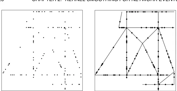
2.1 Point patterns. Left: Non-randomly distributed points. Right:
Ran-domly distributed points on a linear network. . . 26
2.2 Locations of street crimes close to the University of Chicago, US. . 28
2.3 Castell ´on anti-social behaviour during January 2013. . . 29
2.4 Traffic accidents in Medell´ın, Colombia during the year 2016 which caused Left: personal injury, Middle: fatal, Right: property damage. 30
2.5 Traffic accidents in Western Australia during the year 2011. . . 31
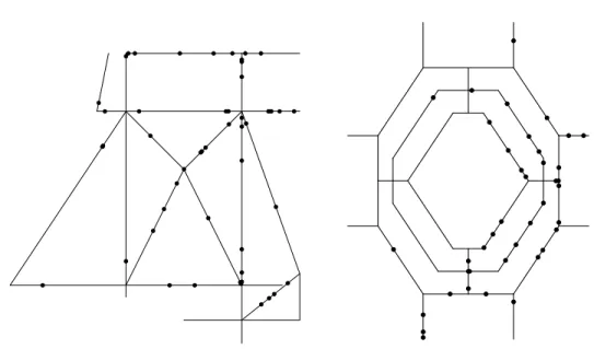
2.6 Realisations of inhomogeneous Poisson processes. Left: with intensity function (2.10) on network L1, Right: with intensity function
(2.12) on network L2. . . 37
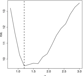
2.7 Bandwidth selection, ISE versus a sequence of bandwidth
smooth-ing parameter σ. . . 38
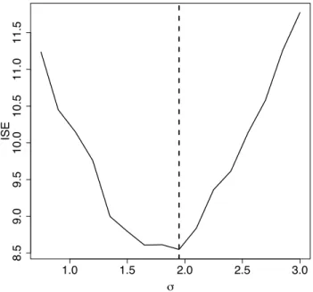
2.8 Intensity visualisation for the pattern on the left hand side of Figure 2.6. Left: true intensity, Middle: adapted Jones-Diggle corrected estimator (2.7) with ISE = 9.57, Right: equal-split discontinuous (2.2) with ISE = 9.66. . . 38 2.9 Bandwidth selection, ISE versus a sequence of bandwidth
xviii INDEX OF FIGURES 2.10 Intensity visualisation for the pattern on the right hand side of Figure
2.6. Left: true intensity, Middle: adapted Jones-Diggle corrected estimator (2.7) with ISE = 8.710, Right: equal-split discontinuous
(2.2) with ISE = 15.384. . . 41
2.11 Bandwidth selection for Chicago crime data. |L| =ˆ Pn
i=1
1/bλJ D
L (xi)
against a sequence of bandwidth smoothing parameter σ (based on feet). Horizontal dashed line shows the total length of the network. 41 2.12 Estimated intensity using adapted Jones-Diggle corrected estimator
for Chicago street crime data with a bandwidth parameter of σ = 650 feet. . . 42 2.13 Bandwidth selection for Castell ´on anti-social behaviour data.
Hori-zontal dashed line shows the total length of the network. . . 43
2.14 Estimated intensity using adapted Jones-Diggle corrected estimator for Castell ´on anti-social behaviour data with a bandwidth parameter of σ = 0.9 km. . . 43 2.15 Kernel estimates of intensity for Chicago data. Perspective views
with height representing the function value. Left: diffusion estimate with bandwidth 125 feet. Right: convolution method with bandwidth
100 feet and uniform correction. . . 49
2.16 Toy example. Simulated point pattern of 4 points on a network of total length 3 units. . . 53 2.17 Kernel estimates of the intensity for the toy example. Left: diffusion
estimate with bandwidth τ = 0.225 units. Middle: convolution estim-ate with uniform correction, bandwidth σ = 0.15 units. Right: con-volution estimate with Jones-Diggle correction, bandwidth σ = 0.15 units. Perspective views with height representing the function value.
Vertical scales are equal. . . 53
2.18 Edge correction denominator cL(u)for the toy network of Figure 2.16
with bandwidth σ equal to 0.015, 0.15 and 1.5 units (left to right). Perspective views with height representing the function value, using different vertical scales. . . 54
INDEX OF FIGURES xix 2.19 Predicted performance on the toy example. Assuming a uniform
Poisson process with intensity 2, and kernel smoothing with band-width 0.15. Top Left: variance (= MSE) of the uniform correction estimator. Top Right: variance of the JonDiggle correction es-timator. Bottom Left: bias of the Jones-Diggle correction estimator, with positive values shown by solid grey colour and negative values by diagonal shading. Bottom Right: MSE of the Jones-Diggle cor-rection estimator. Variance and MSE panels use the same vertical scale. . . 55 2.20 Typical simulated realisations for each of the eight scenarios. Top
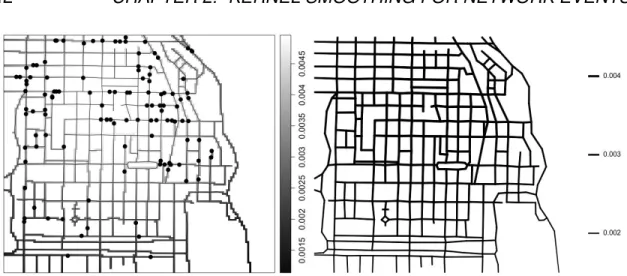
row: Chicago street network. Bottom row: southern part of the city of Perth, extracted from the Western Australian road network. The Gaussian mixture and LGCP realisation scenarios are based on an initial 2D surface defined on W . The diffusion estimate scenario is based on the original data observed on the relevant network.
Simulated realisations all have size n = 500. . . 56
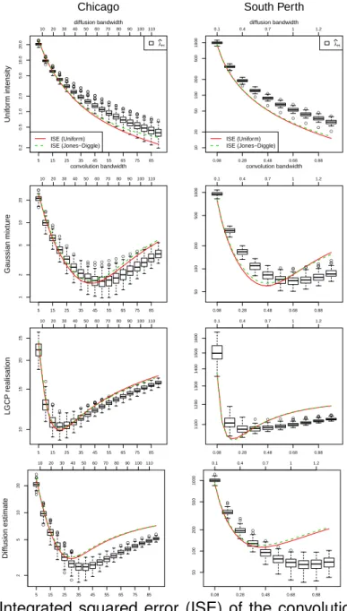
2.21 Integrated squared error (ISE) of the convolution and diffusion es-timators applied to simulated data. Left column: Chicago network; Right column: southern Perth network. Rows represent the four scenarios in Figure 2.20. The bottom horizontal axis in each panel shows the bandwidth σ of the convolution estimator; the top hori-zontal axis shows the bandwidth τ of the diffusion estimator. Box-plots show the numerically computed ISEs for the diffusion estimator. Lines show the theoretically calculated ISEs for bλU
L,con (red, solid)
and bλJ D
L,con(green, dashed). Bandwidths are in feet for Chicago, and
in km for southern Perth. . . 59
2.22 Mean relative execution time per estimate for bλHL relative to both
b
λUL,conand bλJ DL,conacross all four scenarios for the Chicago and
south-ern Perth networks (left and right respectively). . . 61
2.23 Estimated intensity functions for each type of accident in Medell´ın data, using convolution estimator and uniform correction (2.14). Left: property damage, bandwidth 0.36 km; Middle: personal injury, bandwidth 0.36 km; Right: fatal, bandwidth 0.67 km. Intensity values
xx INDEX OF FIGURES 2.24 Estimated relative risk of different types of accidents, relative to
accidents which caused only property damage. Left: personal injury; Right: fatality. . . 65 2.25 Likelihood cross-validation criterion cv(σ) plotted against bandwidth
σ for the kernel estimators of intensity of traffic accidents on the
Western Australian road network. Left: uniform-corrected estimator; the vertical line shows the optimum at σ = 9.1 km. Right: Jones-Diggle estimator; the vertical line shows the optimum at σ = 10.9
km. . . 69
2.26 Fixed-bandwidth estimate of intensity for the accidents on the West-ern Australian road network using the uniform correction with σ = 9.1
km. Intensity values are accidents per km. . . 70
2.27 Fixed-bandwidth estimate of intensity for the accidents on the West-ern Australian road network using the Jones-Diggle correction with
σ = 10.9km. Logarithmic colour map. Intensity values are accidents
per km. . . 71
2.28 Adaptive-bandwidth intensity estimate for the accidents on the West-ern Australian road network using Jones-Diggle correction.
Logar-ithmic colour map. Intensity values are accidents per km. . . 72
2.29 Accidents recorded in the Perth metropolitan area. . . 73
2.30 Adaptive-bandwidth intensity estimate for the accidents in metropol-itan Perth using Jones-Diggle correction. Linear colour map with gamma-corrected colour sequence. Intensity values are accidents
per km. Map is 60 km wide. . . 74
2.31 Accidents recorded in the Central Business District of the city of Perth. . . 76 2.32 Intensity estimate in the Perth CBD using fixed-bandwidth uniform
correction with automatically selected bandwidth σ = 0.091 km.
Intensity values mapped to colours. . . 77
2.33 Intensity estimate in the Perth CBD using fixed-bandwidth uniform correction with automatically selected bandwidth σ = 0.091 km.
Intensity values are proportional to line width. . . 78
INDEX OF FIGURES xxi 2.35 A screenshot of the fixed and adaptive intensity estimates of the
Perth CBD data shown as interactive HEN plots. Accessible at the
URL noted in the text. . . 79
3.1 Estimation error plots for a realisation of a homogeneous Poisson
process X in W = [0, 1]2 with intensity λ = 60. Left: p = 0.2 and
m = 200. Right: p = 1. . . 98
3.2 Estimated bias for bλV
p,m(u) and bλU(u), u ∈ W = [0, 1]2, m = 200,
based on 500 realisations of a homogeneous Poisson process X ⊂
W = [0, 1]2 with intensity λ = 60. From top-left to bottom-right:
b λV
p,m(u)with p = 0.1, 0.3, 0.5, 0.7, 0.9, 1, and bλU(u)using bandwidth
selection (1.12) and (1.13). . . 100
3.3 Estimated variance for bλV
p,m(u) and bλU(u), u ∈ W = [0, 1]2, m =
200, based on 500 realisations of a homogeneous Poisson process
X ⊂ W = [0, 1]2 with intensity λ = 60. From top-left to bottom-right:
b λV
p,m(u)with p = 0.1, 0.3, 0.5, 0.7, 0.9, 1, and bλU(u)using bandwidth
selection (1.12) and (1.13). . . 101 3.4 True intensity and estimation error plots for a realisation of an
inhomogeneous Poisson process on W = [0, 1]2 with intensity
λ(x, y) = |10 + 90 sin(16x)|. Left: p = 0.2 and m = 200. Middle: p = 1, Right: True intensity. . . 102 3.5 Estimated bias for bλV
p,m(u) and bλU(u), u ∈ W = [0, 1]2, m = 200,
based on 500 realisations of an inhomogeneous Poisson process
X ⊆ W = [0, 1]2 with intensity ρ(x, y) = |10 + 90 sin(16x)|. From
top-left to bottom-right: bλV
p,m(u)with p = 0.1, 0.3, 0.5, 0.7, 0.9, 1, and
b
λU(u)using bandwidth selection (1.12) and (1.13). . . 103
3.6 Estimated variance for bλV
p,m(u)and bλU(u), u ∈ W = [0, 1]2, m = 200,
based on 500 realisations of an inhomogeneous Poisson process
X ⊆ W = [0, 1]2 with intensity ρ(x, y) = |10 + 90 sin(16x)|. From
top-left to bottom-right: bλV
p,m(u)with p = 0.1, 0.3, 0.5, 0.7, 0.9, 1, and
b
xxii INDEX OF FIGURES 3.7 True intensity and estimation error plots for a realisation of a
log-Gaussian Cox process in W = [0, 1]2 with mean function (x, y) 7→
log(40| sin(20x)|)and ((x1, y1), (x2, y2)) 7→ 2 exp{−k(x1, y1)−(x2, y2)k/0.1}
as covariance function for the driving random field. Left: p = 0.2
and m = 200. Middle: p = 1. Right: True intensity. . . 107
3.8 Estimated bias for ρbV
p,m(u), u ∈ W = [0, 1]2, m = 200, based on
500 realisations of a log-Gaussian Cox process X ⊆ W = [0, 1]2
where the driving Gaussian random field has mean function (x, y) 7→ log(40| sin(20x)|)and ((x1, y1), (x2, y2)) 7→ 2 exp{−k(x1, y1)−(x2, y2)k/0.1}
as covariance function. From top-left to bottom-right: bλV
p,m(u)with
p = 0.1, 0.3, 0.5, 0.7, 0.9, 1, and bλU(u) using bandwidth selection
(1.12) and (1.13). . . 108 3.9 Estimated variance forρbV
p,m(u), u ∈ W = [0, 1]2, m = 200, based on
500 realisations of a log-Gaussian Cox process X ⊆ W = [0, 1]2
where the driving Gaussian random field has mean function (x, y) 7→ log(40| sin(20x)|)and ((x1, y1), (x2, y2)) 7→ 2 exp{−k(x1, y1)−(x2, y2)k/0.1}
as covariance function. From top-left to bottom-right: bλV
p,m(u)with
p = 0.1, 0.3, 0.5, 0.7, 0.9, 1, and bλU(u) using bandwidth selection
(1.12) and (1.13). . . 109 3.10 True intensity and estimation error plots for a realisation of an
inde-pendently thinned simple sequential inhibition process in W = [0, 1]2
with intensity ρ(x, y) = 450p(x, y), p(x, y) = 1{x < 1/3}|x − 0.02| + 1{1/3 ≤ x < 2/3}|x − 0.5| + 1{x ≥ 2/3}|x − 0.95|, x, y ∈ W . Left:
p = 0.2and m = 200. Middle: p = 1. Right: True intensity. . . 110
3.11 Estimated bias forρbV
p,m(u), u ∈ W = [0, 1]2, m = 200, based on 500
realisations of an independently thinned simple sequential inhibition process in W = [0, 1]2 with intensity ρ(x, y) = 450p(x, y), p(x, y) =
1{x < 1/3}|x − 0.02| + 1{1/3 ≤ x < 2/3}|x − 0.5| + 1{x ≥ 2/3}|x − 0.95|, x, y ∈ W . From top-left to bottom-right: bλV
p,m(u) with p =
0.1, 0.3, 0.5, 0.7, 0.9, 1, and bλU(u) using bandwidth selection (1.12)
INDEX OF FIGURES xxiii 3.12 Estimated variance for ρbVp,m(u), u ∈ W = [0, 1]2, m = 200, based
on 500 realisations of an independently thinned simple sequential inhibition process in W = [0, 1]2 with intensity ρ(x, y) = 450p(x, y),
p(x, y) = 1{x < 1/3}|x − 0.02| + 1{1/3 ≤ x < 2/3}|x − 0.5| + 1{x ≥
2/3}|x − 0.95|, x, y ∈ W . From top-left to bottom-right: bλV
p,m(u)
with p = 0.1, 0.3, 0.5, 0.7, 0.9, 1, and bλU(u)using bandwidth selection
(1.12) and (1.13). . . 112 3.13 Left: Motor vehicle traffic accidents in an area of Houston, US,
during April, 1999. Right: Resample-smoothed Voronoi intensity estimate for m = 200 and p = 0.15. . . 114 3.14 The estimateρbVp,m(u), u ∈ W , m = 200, for p = 0.2 (left) and p = 0.5
(right), together with the locations of 126 pine saplings in a Finnish
forest, within a rectangular window W = [−5, 5] × [−8, 2] (metres). 115
4.1 The motor vehicle traffic accidents in Houston near the university of Houston in 2001 which caused non-incapacitating injury such as bump on the head, abrasions or minor lacerations. Left: The projection of the data onto the network. Right: Cumulative number of data points versus time. . . 129 4.2 Intensity estimates for motor vehicle traffic accidents in Houston.
Left: Intensity estimate of daily hours together with the frequency of accidents per hour (bar plot). Right: Intensity estimate of the
projection onto the network. . . 130
4.3 Estimated second-order characteristics for motor vehicle traffic acci-dents in Houston. Left: Inhomogeneous K-function. Right: Inhomo-geneous pair correlation function. Gray surfaces are envelopes based on 99 simulations and significance level 5% from the com-plete spatio-temporal randomness. . . 130 4.4 Traffic accidents in Medell´ın during the year 2016. Left: The
pro-jection of data onto the network. Right: Cumulative number of data points versus occurrence time. . . 131 4.5 Intensity estimates for traffic accidents in Medell´ın. Left: Intensity
estimate of daily hours together with the frequency of accidents per hour (bar plot). Right: Intensity estimate of the projection onto the network. . . 132
xxiv INDEX OF FIGURES 4.6 Estimated second-order characteristics for traffic accidents in Medell´ın.
Left: Inhomogeneous K-function. Right: Inhomogeneous pair cor-relation function. Gray surfaces are envelopes based on 99 sim-ulations and significance level 5% from complete spatio-temporal randomness. . . 133 4.7 Traffic accidents in the down-town of Eastbourne (UK) in . Left: The
projection of data onto the network. Right: Cumulative number of
data points versus occurrence time. . . 134
4.8 Intensity estimates for traffic accidents in the down-town of East-bourne. Left: Intensity estimate of daily hours together with the frequency of accidents per hour (bar plot). Right: Intensity estimate of the projection onto the network. . . 135 4.9 Estimated second-order characteristics for traffic accidents in the
down-town of Eastbourne. Left: Inhomogeneous K-function. Right: Inhomogeneous pair correlation function. Gray surfaces are point-wise envelopes based on 99 simulations and significance level 5% from complete spatio-temporal randomness. . . 135 5.1 Three consecutive movements of 50 taxis in Beijing, China on Feb
2008per 20 minutes. . . 137
5.2 Single track A1 passed by person A. . . 140
5.3 Classes for trajectory data in the packagetrajectories. Solid arrows
denote inheritance. Arrows show the corresponding slot’s class and slot’s names are displayed using lines accordingly. . . 143 5.4 Simulated random tracks using rTrack. x is random track with all
defaults. y is a random track transformed to a unit box. w is a random track transformed to the box [0, 10] × [0, 10] and z is in a same box as w but with random number of points. . . 146 5.5 Map of the studied area in Beijing, China. . . 148 5.6 Average pairwise distance between taxis in Beijing, China. Left:
Within the period 2 − 8, Feb 2008. Right: During 3-rd of Feb 2008. . 150 5.7 Movement smoothing for taxi data in Beijing, China based on
timestamp = "20 mins" and movements with length longer than 1000 meters. . . 153
INDEX OF FIGURES xxv 5.8 Average length of movements by taxis in Beijing, China versus time
based on timestamp = "20 mins", and movements with length longer than 1000 meters. Left: Within the period 2 − 8 Feb 2008. Right: During the 3-rd of Feb 2008. . . 154 5.9 Estimated intensity function. Left: Beijing. Right: Beijing
metropol-itan area. . . 156 5.10 Chi maps. Left: in the morning, Middle: in the afternoon, Right: at
night. Exact time is reported on top of each plot. . . 158 5.11 Variability area of second-order summary statistics for taxi data in
1
C
HAPTER
1
Introduction
1.1
Data examples
One type of spatial data is when it comes as a set of points which are regularly/ir-regularly distributed within a region of space. Such data might be seen in different contexts such as geo-science, ecology, astronomy, econometrics, criminology, etc. Examples may include trees in a forest, traffic accidents, street crimes, mobile phone calls, animal sightings, or cases of a rare disease. Figure 1.1 shows the location of 86 trees in a forest in New Zealand in a region of approximately 140 by 85 feet. This data was firstly collected by Mark and Esler (1970) and then extracted and analysed by Ripley (2005).
2 CHAPTER 1. INTRODUCTION Figure 1.2 displays the locations of street crimes reported in the period of 25 April to 8 May 2002, in an area of Chicago, US close to the University of Chicago. The original crime map was published in the Chicago Weekly News in 2002 and it has later been analysed by Ang et al. (2012); Baddeley et al. (2015); Moradi et al. (2017); Rakshit et al. (2018). In real world, there are numerous and various events that are strongly constrained by networks, such as traffic accidents and fast-food shops located alongside streets (Okabe and Sugihara, 2012).
Figure 1.2: Locations of street crimes close to the University of Chicago, US. Such patterns, as those shown in Figure 1.1 and 1.2, are called “spatial point patterns” and the locations are referred as “events”. Both displayed datasets
are available in R package spatstat. More of such examples can be found in
Møller and Waagepetersen (2003); Baddeley and Turner (2005); Illian et al. (2008); Gelfand et al. (2010); Okabe and Sugihara (2012); Diggle (2003); Baddeley et al. (2015).
Sometimes the location of objects are recorded over time and according to regular/irregular timestamps. Thus, in this case, we have a set of consecutive points per object and it can be displayed as a track instead of points, and the final pattern is a pattern of tracks which is called “trajectory pattern”. Figure 1.3 shows the Atlantic tropical storm trajectories, in the period of 2009-2012. The dataset is
1.2. SPATIAL POINT PROCESSES ON R2 3 100°W 80°W 60°W 40°W 20°W 0° 10 °N 20 °N 30 °N 40 °N 50 °N 60 °N
Figure 1.3: Atlantic tropical storm trajectories in the period 2009-2012. Datasets in such form are often considered as outcomes of some random mechanism (Baddeley et al., 2015) that a researcher might be interested to discover. For instance, in Figure 1.1 and 1.2, one may be interested to know if events are uniformly distributed over the corresponding region or if there is any particular interaction between them. In Figure 1.3 we may wish to know if the behaviour of objects changes over time.
This chapter is devoted to review the preliminaries that are needed for analysing such datasets. Section 1.2 provides some definitions and reviews some char-acteristics of spatial point processes on R2. A brief introduction to spatial point
processes on linear networks is provided in Section 1.3, and Section 1.4 reviews some preliminaries about trajectory patterns.
1.2
Spatial point processes on R
2A spatial point process is a random countable subset of state space R2.
Through-out this thesis, we only consider finite and simple point processes such that the total number of points has finite second moment, see (Daley and Vere-Jones, 2003, Chapter 5). The outcome of such process is called a spatial point pattern which is
4 CHAPTER 1. INTRODUCTION a dataset giving the observed spatial locations of things or events. However, in practice, we only observe some points placed in a bounded observation window W ⊂ R2. Hereafter, we denote point processes with capital letters such as X, Y, . . .
and the corresponding point patterns as x, y, . . .. For any arbitrary bounded subset A ⊂ R2, its cardinality, N (X ∩ A), is the number of points falling in A ⊂ R2. For
any point process X,
E[N (X ∩ A)] = Z
A
λ(u)du, u ∈ R2, (1.1)
where λ(·) is called intensity function which governs the behaviour of the underlying point process and shows how it uses the corresponding space. When studying point patterns, one of the very first steps is to investigate the behaviour of the intensity function. Intuitively, the intensity function λ(u) is the expected number of points per unit area in the vicinity of location u ∈ R2. If the intensity function λ(·)
is constant, then the point process X is called homogeneous, otherwise it is an
inhomogeneous point process on R2. Equation (1.1) might be extended to higher
orders, e.g. for every subsets A, B ⊂ R2,
E [N (X ∩ A)N (X ∩ B)] = Z A Z B λ2(u, v)dudv, u, v ∈ R2, (1.2)
where λ2(·, ·) is the second-order product density function of X.
A spatial point process X on state space R2 is stationary if its distribution is
invariant under translations, i.e. for any arbitrary point a ∈ R2 the distributions of
X and X + a are the same (Møller and Waagepetersen, 2003). Although such
aspect might add much to the convenience, in practice we usually face datasets with lack of stationarity. The point process X is second-order intensity-reweighted stationary if the second moment measure
M (A, B) = E X xi∈X∩A X xj∈X∩B 1 λ(xi)λ(xj) , (1.3)
is second-order stationary, i.e. M (A, B) = M (A + a, B + a) for all a ∈ R2(Baddeley
et al., 2000). The point process X is isotropic if its distribution is invariant under rotations around the origin (Møller and Waagepetersen, 2003).
We denote a realisation of a point process X with n points as x = {x1, x2, . . . , xn}
1.2. SPATIAL POINT PROCESSES ON R2 5
one realisation to another one. For any non-negative and measurable function f on R2, the intensity function λ(·) satisfies
E X x∈X f (x) = Z R2 f (u)λ(u)du. (1.4)
Equation (1.4) has been widely used in the literature of point processes and it is called Campbell’s formula and it can be extended to higher orders so that e.g. for second-order is of the form
E 6= X x,y∈X f (x, y) = Z R2 Z R2
f (u, v)λ2(u, v)dudv, (1.5)
where
6=
P means that the sum is over distinct pair of points.
1.2.1
Point process models
A very popular and important model for point processes is the Poisson point processes which satisfies the following conditions:
1. N (X ∩ A) follows a Poisson distribution with parameterR
Aλ(u)du.
2. Given N (X ∩ W ) = n, events in the window W constitute an independent random sample from the uniform distribution over W .
3. For any finite number of disjoint subsets Ai ⊂ W (i = 2, . . . , m), the random
variables N (Ai∩ W ) are independent.
Such conditions lead to have no interaction amongst the events so that they do not tend to either happen closely or distantly. Such model might bring ease, however as listed above, a crucial assumption of Poisson point process models is that points are independent of each other, which does not seem to be an appropriate assumption when analysing real data. Due to simplicity and having known values for summary statistics (see Section 1.2.4), Poisson processes are usually used as a benchmark for model selection. They are also used to build more complex and flexible models such as Cox point processes which are clustered due to an environmental random heterogeneity (Møller and Waagepetersen, 2003). The source of such environmental heterogeneity might itself be stochastic in nature (Diggle, 2003).
6 CHAPTER 1. INTRODUCTION A Cox point process is a Poisson process when its intensity function is con-sidered as a realisation of a random field, i.e. doubly stochastic behaviour is here considered. This being said, the conditional distribution of a Cox process given the underlying random field is a Poisson point process. For details of random fields see Adler (1981). A Cox process is assumed stationary if the underlying random field is stationary. For a broad introduction to Cox processes, see Møller and Waagepetersen (2003, Chapter 5).
In some real applications events might tend to not get close to each other more than a particular distance. A nice example in biology is provided in (van Lieshout, 2000, Chapter 2) in which in a pattern of cells, no nucleus can be closer to other nucleus more than a particular distance. A family of point processes which might cover such behaviour is Markov point processes that considers a density for point processes with respect to a Poisson process. For key references to Markov point processes see van Lieshout (2000) and Møller and Waagepetersen (2003).
1.2.2
Intensity estimators
One of the very first steps to get into the behaviour of the point pattern x is to study the intensity function λ(·) since it might reveal the distribution of the underlying point process X. If the point process X has constant intensity function, then
b
λ = n(x)
|W |, (1.6)
is an unbiased estimator for the intensity function λ(·) where n(x) is the number of points of pattern x and |W | is the volume of window W . However, in practice, this assumption seems hard to be realistic.
1.2.2.1 Kernel smoothing
Kernel smoothing is usually the most popular method to estimate the intensity function. The uncorrected kernel estimator is of the form
b λ0(u) = n X i=1 κ(u − xi), u ∈ W, (1.7)
where the kernel κ is a probability density function on R2. This estimator generates
1.2. SPATIAL POINT PROCESSES ON R2 7
outside the window. In order to improve the efficiency of the estimator (1.7), Diggle (1985) introduced an uniformly corrected version as
b λU(u) = 1 eW(u) n X i=1 κ(u − xi), u ∈ W, (1.8) where eW(u) = Z W κ(u − v)dv, (1.9)
is the mass of the kernel centred at u that falls inside the window. The correction (1.9) is often called the “uniform” edge correction, because it ensures that bλU(·)
is a pointwise unbiased estimator when the true intensity is uniform. That is, if λ(u) ≡ λ > 0, then E[bλU(u)] ≡ λ. Jones (1993) proposed an alternative estimator
as b λJ D(u) = n X i=1 κ(u − xi) eW(xi) , u ∈ W, (1.10)
often confusingly called the “Diggle correction” in the spatial statistics literature. We shall call it the “Jones-Diggle” correction. This estimator conserves total mass, that is,
Z
W
b
λJ D(u)du = n. (1.11)
The initial difference between (1.8) and (1.10) is the way they apply the correction that makes other differences in terms of efficiency. The degree of smoothing in the estimators above strongly depends on the smoothing parameter bandwidth. A small bandwidth might result in under-smoothing while a large bandwidth may over smooth the intensity. Moreover, small bandwidth results in small bias and large variance, while large bandwidth makes larger bias and less variation. For more details see Baddeley et al. (2015, Chapter 6).
However, to compute the aforementioned intensity estimators, a smoothing bandwidth parameter needs to be picked previously. Bandwidth selection process has always been a challenge when estimating intensity functions using kernel smoothing methods. Prior researches such as Diggle (1985); Silverman (1986); Berman and Diggle (1989); Scott (1992); Wand and Jones (1994); Jones et al. (1996); Loader (1999) on bandwidth selection method shows that we are unlikely to find a data-based method which performs uniformly well. Diggle (1985) aimed at
8 CHAPTER 1. INTRODUCTION finding a proper choice of bandwidth by minimising the “mean square error ” when the underlying point process is assumed to be a stationary Cox process. However, the very common method to find a proper bandwidth might be “leave-one-out” cross validation based on the Poisson point process likelihood in which it selects a bandwidth which maximises
CV (σ) = n X i=1 log(bλ−iσ (xi)) − Z S b λσ(u)du, (1.12)
where σ is bandwidth and bλ−iσ (xi)is the intensity estimator at data point xiwhen we
have excluded xifrom the point pattern in question. In other words, the contribution
of xi in the sum in equations (1.8) and (1.10) has been omitted. For estimators
which provide mass conservation such as estimator (1.10), we might exclude the integral part in the cross validation since it is equal to the number of data points.
A simple way to at least reach a range of trial values of σ is the Scott’s rule of thumb (Scott, 1992) according to which, j-th Cartesian coordinate (j = 1, 2) should
be smoothed with bandwidth σj = cn,2sj where sj is the sample standard deviation
of the j-th Cartesian coordinate values for the data points, and cn,2 = (4n)−1/6
where n is the number of data points.
Cronie and van Lieshout (2018) defined a non-model-based approach to choose the bandwidth based on the fact that
E X x∈X∩W 1 λ(x) = Z W 1 λ(u)λ(u)du = |W |, u ∈ W. (1.13)
Equation above results from using the Campbell formula (1.4). Cronie and van Lieshout (2018) considered a proper choice of the bandwidth as the one which minimises the discrepancy between the total volume of the corresponding window
W and the left side of equation (1.13) when λ(x) is replaced by its estimator.
An extensive comparison with other methods based on “leave-one-out” cross validation and “mean square error ” is also provided by Cronie and van Lieshout (2018).
1.2.2.2 Adaptive kernel intensity estimators
Intensity estimators such as (1.7),(1.8) and (1.10) are based on “fixed-bandwidth smoothers”, i.e. same kernel and the same bandwidth are considered to calculate
1.2. SPATIAL POINT PROCESSES ON R2 9
the estimator at different spatial locations in which local effects on the estimation might be neglected. Especially, a fixed smoothing bandwidth is unsatisfactory when the true intensity varies greatly across the spatial domain, because it is likely to cause over-smoothing in the high-intensity areas and under-smoothing in the low intensity areas. Kernel estimators such as (1.7),(1.8) and (1.10) might suffer from sharp boundaries between areas with high and low intensity, because this boundary will be smoothed out (Baddeley et al., 2015). In such situations, adaptive (variable-bandwidth) kernel estimation can perform substantially better (Abramson, 1982; Hall and Marron, 1988) where an alternative is to allow the degree of smoothing to be adapted to local smoothing requirements. Adaptive versions of (1.8) and (1.10) are in the form of
b λUa(u) = 1 eW(u, σ(u)) n X i=1 κσ(xi)(u − xi), u ∈ W, (1.14) and b λJ Da (u) = n X i=1 κσ(xi)(u − xi) eW(xi, σ(xi)) , u ∈ W, (1.15)
where σ(·) is the spatially-varying bandwidth function (Marshall and Hazelton, 2010; Rakshit et al., 2018). Although estimator (1.14) is analogous to the estimator (1.8), it does not retain the same unbiasedness property. However, estimator (1.15) still provides mass conservation. Estimators (1.14) and (1.15) take longer time to be computed.
1.2.2.3 Adaptive Voronoi estimators
The Voronoi cell associated with a particular data point xi is the area of R2
which is closer to xi than any other points when the observed point pattern
x = {x1, x2, · · · , xn} is distributed over W ⊂ R2. We then denote a Dirichlet cell as
Vxi = Vxi(x, W ) = {u ∈ W : ||u − xi|| ≤ ||u − xj|| for all xj ∈ x \ {xi}}, (1.16) where || · || stands for the Euclidean distance. Finding the Dirichlet cell of all data points results in a set of non-overlapping, disjoint and convex polygons which build a Voronoi tessellation out of the observed point pattern. The adaptive Voronoi intensity estimator bλ(u)at location u ∈ W is then the reciprocal size of Vu(x, W ),
the cell where u belongs to. This estimator is unbiased when the underlying point process is homogeneous, conserves mass and performs well when there
10 CHAPTER 1. INTRODUCTION are abrupt changes in the intensity of observed data (Baddeley et al., 2015, Chapter 6). However, it generates a huge variance (Barr and Schoenberg, 2010; Moradi et al., 2018a). Apparently, it was first introduced by Brown (1965) and Ord (1978). Ebeling and Wiedenmann (1993) used Voronoi estimators to study spatial concentration of photons locally. Other applications such as estimating neuronal density can be found in Duyckaerts et al. (1994); Duyckaerts and Godefroy (2000). Barr and Schoenberg (2010) investigate statistical properties of such intensity estimator when the underlying point process is supposed to be an inhomogeneous process. Under particular conditions, they also discussed being approximately ratio-unbiased when the underlying point process is an inhomogeneous Poisson process. Moreover, this Voronoi technique has also been used in statistical seismology (Ogata, 2011; Baddeley et al., 2015).
1.2.3
Relative risk
Sometimes the point pattern in question contains points with different marks. A very known example might be a spatial case-control study in which some points play the role of control and others the spatial locations of a set of disease cases. The spatially varying risk of the case study might be measured by the ratio of the intensity function of the two point processes (Bithell, 1991; Kelsall and Diggle, 1995a,b; Diggle, 2003; Baddeley et al., 2015).
Consider there are two different observed point patterns x and y, generated by point processes X and Y , respectively. The relative risk of the two point process is of the form
ρ(u) = logλX(u) λY(u)
, u ∈ S, (1.17)
where λX(u), λY(u)are the intensity functions of the underlying point processes X
and Y , respectively. However, in practice, ρ needs to be estimated and it demands
to estimate λX(u)and λY(u)individually. An enough good estimate of ρ provides
us with the spatially-varying relative frequency of each type of points.
The very first idea to estimate ρ is to use the plug-in estimator based on kernel
estimators of λX(u) and λY(u). Here, the challenge is to choose bandwidth
smoothing parameter. As the two patterns x and y are generated by two different
point process, one might estimate λX(u) and λY(u) using different bandwidth
1.2. SPATIAL POINT PROCESSES ON R2 11
(1995a) suggest to use equal bandwidths. Davies et al. (2016) show that using different bandwidth parameters might lead in potentially misleading methodological artefacts in the resulting estimates. Different bandwidth selection methods for the optimal estimation of relative risk ρ are discussed in Lawson and Williams (1993); Kelsall and Diggle (1995a,b); Diggle et al. (2005); Hazelton (2008); Davies and Hazelton (2010); Davies (2013); Davies and Baddeley (2018). An overview of various estimators and bandwidth selection methods is also provided by Davies et al. (2018).
Some jointly optimal bandwidth selection methods including minimising the approximate mean integrated squared error (MISE) of the log-transformed risk surface (Kelsall and Diggle, 1995a), a weighted-by-control MISE (Hazelton, 2008) and a crude plug-in approximation to the asymptotic MISE (Davies, 2013) are
implemented in R packagesparr (Davies et al., 2018).
1.2.4
Second-order summary statistics
In order to get into the type of the interaction between events, we might aim at studying the correlation between events. In the literature of point processes, the type of such correlation can be determined by using summary statistics. Thinking of correlation, the first thing that comes to mind might be using “second-moment” quantities which are built based on pairs of points. Note that to be able to calculate the second-moment quantities we need to estimate the first moment previously. We now review some summary statistics in point process literature.
A summary function that is mostly used to analyse the spatial correlation of point events is K-function which is firstly introduced by Ripley (1977). Considering
X a stationary point process on R2 with constant intensity λ, Ripley (1977) defined
the K-function so that λK(r) is the expected number of further points of X lying within a distance r of a typical point of X, i.e. for any location u ∈ R2,
K(r) = 1
λE [N (X ∩ b(u, r) \ {u}) | u ∈ X] , (1.18)
where b(u, r) is a disc of radius r centred at u. The expectation in (1.18) is formally defined as an expectation with respect to the Palm distribution of X at u, see Daley and Vere-Jones (2003) and Møller and Waagepetersen (2003). Since X is stationary, this expectation does not depend on the choice of location u. For
12 CHAPTER 1. INTRODUCTION second-moment quantity, K(r) = 1 λ2|B|E X xi∈X∩B X xj∈X 1{0 < kxj− xik ≤ r} , (1.19)
so that λ2|B| K(r) is the expected number of ordered pairs of distinct points (x
i, xj)
lying at most r units apart, with the first point xi falling in B. Again, the stationarity
of X implies that the right hand side of (1.19) does not depend on the choice of B.
When a realisation of X is observed inside the window W ⊂ R2, giving a point
pattern x = {x1, . . . , xn} of points xi ∈ W , the estimator of K(r) is of the form
b K(r) = |W | n(n − 1) X i X j6=i 1{kxi− xjk ≤ r}eW(xi, xj, r), (1.20)
where eW(xi, xj, r)is a correction for edge effect bias (Baddeley et al., 2015).
Note that (1.20) is a biased estimator of K(r). The double sum on the right
of (1.20) is an unbiased estimate of λ2|W |K(r) for any stationary point process.
The denominator n(n − 1) effectively serves as an estimator of λ2|W |2, but is only
unbiased if X is a Poisson process. Writing bK(r) = A/B where A is the double
sum in (1.20) and B = n(n − 1)/|W |, we have E[A]/E[B] = K(r) if X is a Poisson
process. Under reasonable assumptions, bK(r)is a consistent estimator of K(r).
In practice the bias is usually small when r is not too large (Moradi et al., 2018d). However, when analysing real data, it rarely happens to have the point process in question stationary. Thus, the empirical K-function might be misleading if applied to point pattern data which are spatially inhomogeneous. By developing an analogue of K-function (1.19), Baddeley et al. (2000) extended the K-function to the cases in which the pattern is spatially inhomogeneous. For second-order intensity-reweighted stationary point processes, they defined the K-function as
Kinhom(r) = 1 |B|E X xi∈X∩B X xj∈X 1{0 < kxj − xik ≤ r} λ(xi)λ(xj) , (1.21)
which does not depend on the choice of B. Baddeley et al. (2000) further proposed the following pointwise unbiased estimator
b Kinhom(r) = 1 |W | X i X j6=i 1{kxi− xjk ≤ r}eW(xi, xj, r) λ(xi)λ(xj) , (1.22)
1.3. SPATIAL POINT PROCESSES ON LINEAR NETWORKS 13 where similar to (1.20), eW(xi, xj, r)is an edge correction. In the literature, different
edge corrections have been developed and an overview and comparison can be found in Gabriel (2014).
In practice, however, λ(·) needs to be estimated as it is not known previously. Thus, an estimate of λ(·) is needed in advance to compute (1.22). Notwithstanding,
replacing λ(·) by bλ(·) in (1.22) makes it severely under-biased which might be
caused from the bias of the intensity estimator. Baddeley et al. (2000) suggested to use the “leave-one-out” kernel smoother to estimate the intensity function which seems to provide a better estimator for the K-function.
Regardless of homogeneity, for Poisson point processes K(r) = πr2. Values
larger than πr2 indicate clustering behaviour while values smaller than πr2 point
out repulsion. Another second-order summary statistic which has been frequently used is the pair correlation function that is defined as
g(u, v) = λ2(u, v)
λ(u)λ(v), u, v ∈ R
2. (1.23)
For Poisson processes, g(·, ·) = 1 as λ2(·, ·) = λ(·)λ(·). Values larger than one
indicate clustering behaviour whereas values less than one show repulsion. This
comes from the fact that values larger than one mean λ2(·, ·) > λ(·)λ(·) which
shows the tendency of points to be closer to each other. With the assumption that g is translation invariant, i.e. g(u, u + h) = g0(h)for some function g0 : R2 → [0, ∞),
then X is second-order intensity-reweighed stationary and
Kinhom(r) =
Z
b(o,r)
g0(h)dh, (1.24)
where b(o, r) denotes a disc centred at origin with radius r > 0.
1.3
Spatial point processes on linear networks
The last decade witnessed an extraordinary increase in interest in the analysis of network related data within numerous disciplines. This pervasive interest is partly caused by a strongly expanded availability of network data. In the spatial statistics field, there are numerous real examples such as the location of traffic accidents, geo-coded locations of crimes or anti-social behaviour events in the streets of cities that need to restrict the support of the underlying process over
14 CHAPTER 1. INTRODUCTION such linear networks to set and define a more realistic scenario. Network events can be categorised to on-network events such as traffic accidents which inherently happen on street networks and alongside-network events such as street crimes on side-walk which are usually committed alongside to street networks. The inherent geometry of a linear network makes the analysis of spatial point patterns as a different story with respect to the analysis of such patterns occurring on planar regions (reviewed in Section 1.2). For example, measuring distance between events play an important role when events are living on a linear network.
A nice introduction on spatial analysis along networks can be found in Okabe and Sugihara (2012). Following, we provide the extension of spatial point processes to network events.
1.3.1
Linear networks
A line segment in the plane with endpoints u and v can be written in a parametric
form as [u, v] = {tu + (1 − t)v : 0 ≤ t ≤ 1} with u, v ∈ R2. A linear network L can
be defined as the union of a finite collection of line segments embedded in the plane (Ang et al., 2012). The endpoints of the segments are called nodes and the degree of a node n (denoted by δ) is the number of line segments that share the same node (Okabe and Sugihara, 2012). The total length of all line segments in
Lis denoted by |L|. The distance between two points u and v in the network L
is usually computed by the shortest-path distance dL(u, v)which is the minimum
of the length of all possible paths between u and v. However, different possible distances have been discussed in Rakshit et al. (2017); Anderes et al. (2017).
The disc of radius r > 0 centred at the point u ∈ L is given by bL(u, r) =
{v ∈ L : dL(u, v) ≤ r} which includes all points within a shortest-path distance
less than r, and its relative boundary ∂bL(u, r)is the set of points lying exactly r
units away from u. Moreover, the circumference m(u, r) is the number of points in the relative boundary with centre at u and radius r which are on the linear network L, i.e. m(u, r) = #{∂bL(u, r) ∩ L}. The circumference is finite for r < ∞
and m(u, ∞) = ∞ by convention. In addition, R(L) is the largest value so that
m(u, r) 6= 0for all events u ∈ X and all r ≤ R(L) (for more details see (Baddeley
et al., 2015, Chapter 17)).
Similar to planar point processes, a point process X on a linear network L
1.3. SPATIAL POINT PROCESSES ON LINEAR NETWORKS 15 modifications, most of the provided details in Section 1.2 are also valid for network events. For instance, the intensity measure (1.1) is in the form
E[N (X ∩ A)] = Z
A
λ(u)d1u, u ∈ L, (1.25)
where d1udenotes one-dimensional integration over the line segment (Federer,
1996; Ang et al., 2012), λ(·) is considered as the intensity function of X and A ⊂ L. Here, λ(u) gives the expected number of points per unit length of the network in the vicinity of location u. For any non-negative and measurable function f on L, Campbell’s formula is of the form
E X x∈X f (x) = Z L f (u)λ(u)d1u. (1.26)
Surprisingly, intensity estimation on a network of lines, such as a road network, seems to be a complicated task. Several techniques published in the literature, in geography and computer science, have turned out to be erroneous in which some of the existing techniques are also computationally expensive (Xie and Yan, 2008; Okabe et al., 2009; McSwiggan et al., 2017; Moradi et al., 2017). In Chapter 2, we will review the current intensity estimations together with their advantages and/or disadvantages. Some new intensity estimators are also proposed in Chapters 2 and 3.
Due to the nature of networks, there is still no clear picture of how stationarity can be defined on linear networks. For example, using the classical shift transformation, there is no guarantee if the point will still live on the network after transformation. Baddeley et al. (2017) considered some popular procedures to construct point patterns on networks and pointed out that models are no longer stationary when distance is measured using the shortest-path distance. Having no clear picture of an applicable transformation method on networks might make some restriction of developing more complex models and summary statistics such as higher order ones (van Lieshout, 2011). However, Anderes et al. (2017) developed some parametric classes of covariance functions for linear networks, defined on the nodes and edge points. Their covariance functions are also isotropic i.e. they only depend on the geodesic distance or resistance metric which was considered in Anderes et al. (2017). The resistance metric here is an extension of the resistance
16 CHAPTER 1. INTRODUCTION metric developed in electrical network theory (Anderes et al., 2017). van Lieshout (2017) also defined nearest-neighbour point processes on linear networks.
1.3.2
Second-order summary statistics
Another consequence of considering a linear network as a state space for the point process X is coming up when dealing with summary statistics such as K-function and pair correlation function. Okabe and Yamada (2001) adapted the K-function to the linear network by only replacing the Euclidean distance by shortest-path distance as b Knet(r) = |L| n(n − 1) n X i=1 X j6=i 1{dL(xi, xj) ≤ r}. (1.27)
However, this modification was affected by the geometry of the linear network and
its interpretation was not easy. The bKnet can be reformed as a Palm expectation
and then it discloses that bKnet depends on locations, even for Poisson processes,
see Ang et al. (2012). Thus, there is no simple benchmark to measure the
deviation from Poisson processes. Moreover, no connection between bKnet and
pair correlation function could be provided.
Knowing this, Ang et al. (2012) proposed a modification as
b KL(r) = |L| n(n − 1) n X i=1 X j6=i 1{dL(xi, xj) ≤ r} m(xi, dL(xi, xj)) , (1.28)
for 0 ≤ r ≤ R(L). The m(xi, dL(xi, xj)) in the denominator of (1.28) is
some-how playing the role of an edge correction by adding a contribution from each pair of points. This is actually analogous to the isotropic edge correction, since m(xi, dL(xi, xj)) is a measure of the size of the boundary of the ball of radius
dL(xi, xj)centred at xi (Ripley, 1977; Ang et al., 2012). For the point process X
on the linear network L with constant intensity λ > 0, Ang et al. (2012) defined the geometrically corrected K-function as
KL(u, r) = 1 λE " X i 1{dL(u, xi) ≤ r} m(u, dL(u, xi)) u ∈ X # , (1.29)
and called X second-order pseudostationary if KL(u, r) does not depend on