Universidade de Aveiro 2018
Departamento de Biologia
Ana Maria
Simões do Paço
Biodegradation of microplastics: Optimization and
Scale up
Biodegradação de microplásticos: Otimização e
Aumento da escala
DECLARAÇÃO
Declaro que este relatório é integralmente da minha autoria, estando devidamente referenciadas as fontes e obras consultadas, bem como identificadas de modo claro as citações dessas obras. Não contém, por isso, qualquer tipo de plágio quer de textos publicados, qualquer que seja o meio dessa publicação, incluindo meios eletrónicos, quer de trabalhos académicos.
Universidade de Aveiro 2018 Departamento de Biologia
Ana Maria
Simões do Paço
Biodegradation of microplastics: Optimization and
Scale up
Biodegradação de microplásticos: Otimização e
Aumento da escala
Dissertação apresentada à Universidade de Aveiro para cumprimento dos requisitos necessários à obtenção do grau de Mestre em Biologia Aplicada, realizada sob a orientação científica da Doutora Teresa Rocha Santos, Investigadora Principal do Departamento de Química e do Centro de estudos do Ambiente e do Mar (CESAM), Universidade de Aveiro, e do Doutor João Pinto da Costa, Investigador em Pós-Doutoramento do Departamento de Química e do CESAM, Universidade de aveiro.
Este trabalho foi parcialmente financiado com apoio do CESAM (UID/AMB/50017) e da FCT/MEC através de fundos nacionais e co-financiado pelo FEDER, dentro do acordo da parceria PT2020 e Compete2020.
Foi também finaciado por fundos nacionais da FCT/MEC (PIDDAC)
no âmbito do projeto
IF/00407/2013/CP1162/CT0023 e co-financiamento pelo FEDER, no âmbito do acordo de parceria
PT2020
POCI-01-0145-FEDER-028740.
Apoio financeiro da FCT através
da bolsa
SFRH/BPD/122538/2016 no
âmbito dos fundos POCH, co-financiados pelo Fundo Social
Europeu e pelos Fundos
o júri
presidente Professora Doutora Maria Adelaide de Pinho Almeida
professora auxiliar com agregação do Departamento de Biologia da Universidade de Aveiro
Doutora Ana Cristina Cardoso Freitas Lopes de Freitas
investigadora principal do Centro de Biotecnologia e Química Fina, Universidade Católica Portuguesa do Porto
Doutora Teresa Alexandra Peixoto da Rocha Santos
investigadora principal do Departamento de Química e do Centro de Estudos do Ambiente e do Mar (CESAM), Universidade de Aveiro
agradecimentos Agradeço em especial, à Doutora Teresa Rocha Santos pela orientação científica, ensinamentos, apoio e disponibilidade durante a realização deste trabalho.
Ao Doutor João Costa, pela partilha de conhecimentos e sugestões e pela sua disponibilidade.
Ao Professor Armando da Costa Duarte, pela disponibilidade para esclarecimento de dúvidas e pelos ensinamentos.
Ao Professor Armando Silvestre, ao Professor Jorge Saraiva e à Doutora Andreia Sousa, pela disponibilidade durante a realização do trabalho.
À Doutora Ana Violeta Girão, por toda a disponibilidade e pelas explicações e fotos incríveis.
À Vanessa Reis e à Jéssica Jacinto, por todo o apoio e ajuda, tanto no laboratório, como fora dele.
À Ana Catarina Latães e à Inês Romão, pela ajuda na realização dos trabalhos laboratoriais.
Aos companheiros de tese, por toda a compreensão e apoio nestes últimos meses.
palavras-chave Zalerion maritimum, Nia vibrissa, fungo, biodegradação, microplástico, polietileno, poli(2,5- furanodicarboxilato de etileno), bioplástico, FTIR-ATR, SEM
resumo O lixo marinho, em especial, os plásticos de pequenas dimensões,
é uma das maiores ameaças ao ecossistema marinho. A presença destes microplásticos tem vindo a aumentar nos últimos tempos, devido ao uso indiscriminado de plástico pela população humana e à falta de políticas para a sua gestão.
Assim, é necessário encontrar maneiras de mitigar os seus impactos ou mesmo reduzir a sua presença. A biodegradação surge como uma solução promissora para este problema.
Neste trabalho, com o objetivo de desenvolver um processo de biorremediação, o potencial de biodegradação, de microplásticos de polietileno, do fungo Zalerion maritimum é explorado. Através da otimização do meio de cultura, por “Central composite design” e por “Uniform design”, foi possível obter maiores taxas de remoção de microplásticos e verificar que o extrato de malte é o constituinte do meio mais relevante neste processo. Pelo aumento da escala foi possível verificar que mesmo num ambiente menos controlado o fungo biodegrada microplásticos.
Além disso, foi também testada a resposta do fungo Zalerion maritimum e do fungo Nia vibrissa, quando expostos ao poli(2,5- furanodicarboxilato de etileno) e foi possível verificar que ambos os fungos parecem ter a capacidade de biodegradar este micro(bio)plástico.
keywords Zalerion maritimum, Nia vibrissa, fungus, biodegradation,
microplastics, polyethylene, poly(ethylene2,5-furandicarboxylate), bioplastic, FTIR-ATR, SEM
abstract Marine litter, specifically small plastic particles, is one of the major threats to the marine ecosystem. The presence of these microplastics has been increasing over the last few years due to their indiscriminate use and lack of polices for their management.
Thereby, it is necessary to encounter new ways to mitigate their impacts or even reduce their presence. Biodegradations is a promising solution to this problem.
In this work, with the objective of developing a bioremediation process the potential of Zalerion maritimum, to biodegrade polyethylene microplastics, is exploited.
Through optimization of the biodegradation medium, by Central composite design and by Uniform design, was possible to obtain higher percentages of microplastics removal and verify that malt extract was the most relevant compost medium to the process. By scale up it was possible to verify that in a less controlled medium the biodegradation of microplastics still occur.
In addition, the response of the fungi Zalerion maritimum and Nia
vibrissa to exposure to poly(ethylene2,5-furandicarboxylate) has
also been studied and it was possible to conclude that these fungi seems to have the capacity of biodegrade this micro(bio)plastic.
Contents
List of figures ... iii
List of tables ... iv
List of abbreviations ... v
1. Introduction ... 1
1.1. Plastics in the marine environment ... 1
1.2. Degradation of plastics – types and definition ... 8
1.2.1. Abiotic Degradation ... 8 1.2.1.1. Chemical ... 8 1.2.1.2. Mechanical ... 8 1.2.1.3. Thermal ... 8 1.2.1.4. Photodegradation ... 9 1.2.2. Biodegradation ... 9
1.2.2.1. Microorganisms involved in biodegradation ... 11
2. Optimization of the experimental conditions for the biodegradation of polyethylene microplastics by marine fungi ... 14
2.1. Introduction ... 14
2.1.1. Uniform Design (UD) ... 15
2.1.2. Central Composite Design (CCD) ... 15
2.1.3. Zalerion maritimum ... 16
2.1.4. Polyethylene (PE) ... 18
2.2. Materials and Methods ... 20
2.2.1. Microplastics ... 20
2.2.2. Microorganism ... 21
2.2.3. Design of experiments and Statistical analysis ... 21
2.2.3.1. Uniform Design ... 21
2.2.3.2. Central Composite Design ... 22
2.2.4. Culture medium ... 22
2.2.5. Experimental conditions ... 24
2.3. Results and discussion ... 25
2.3.1. Effect of different medium compounds on polyethylene’s biodegradation ... 26
2.3.1.1. Uniform Design ... 26
2.3.1.2. Central composite design ... 30
2.3.2. Optimization of the culture medium composition ... 34
2.5. Conclusion ... 35
3. Biodegradation of polyethylene microplastics by marine fungi: Scale up ... 36
3.1. Introduction ... 36
3.2. Materials and methods ... 36
3.2.1. Microorganism and microplastics ... 36
3.2.2. Culture medium ... 36
3.2.3. Experimental conditions ... 37
3.2.4. Microplastics treatment ... 38
3.2.5. Techniques used to analyze the microplastics ... 38
3.3.1. Impact of the microplastics on the growth rate of Zalerion maritimum ... 39
3.3.2. Changes in biodegradation with microplastics size ... 44
3.3.3. Biodegradation in an optimized medium ... 47
3.4. Conclusion ... 50
4. Removal of bioplastics of Poly(ethylene2,5-furandicarboxylate) using marine fungi ... 51
4.1. Introduction ... 51
4.1.1. Nia vibrissa ... 51
4.1.2. Bioplastics ... 52
4.2. Materials and methods ... 53
4.2.1. Microplastics ... 53
4.2.2. Microorganisms ... 54
4.2.3. Culture medium ... 54
4.2.4. Experimental conditions ... 54
4.2.5. Techniques used to analyze the microplastics ... 55
4.1. Results and discussion ... 56
4.1.1. First experiment to assess the capacity of Zalerion maritimum to biodegrade PEF microplastics ... 56
4.1.2. Comparison between Zalerion maritimum and Nia vibrissa capacity of biodegrade PEF microplastics ... 59
4.2. Conclusion ... 62
5. Conclusions and future perspectives ... 63
6. References ... 65
7. Appendix A ... 77
List of figures
Figure 1 – Schematic presentation of the sources of microplastics1 from Maphoto/Riccardo Pravettoni,
available at http://www.grida.no/resources/6929. ... 2
Figure 2 – Microplastics’ pathways into the ocean1 from Maphoto/Riccardo Pravettoni, available at http://www.grida.no/resources/6921. ... 3
Figure 3 – Representation of the marine currents and the marine gyres1 from Maphoto/Riccardo Pravettoni, available at http://www.grida.no/resources/6913. ... 4
Figure 4 – Model of the amount of microplastics present in the marine environment and the mismanaged plastic particles available to enter in the oceans, retrieved from Zalasiewicz et al.15 with the permission of Elsevier. ... 5
Figure 5 – Schematic representation of the relation between microplastics and the marine animals1 from Maphoto/Riccardo Pravettoni, available at http://www.grida.no/resources/6904. ... 6
Figure 6 - Representation of the bioaccumulation effect of the microplastics1 from Maphoto/Riccardo Pravettoni, available at http://www.grida.no/resources/6917. ... 6
Figure 7 - Schematic presentation of the biodegradation’s mechanisms, retrieved from Mueller et al.42 with the permission of Elsevier ... 11
Figure 8 – Photos from the different forms that Zalerion maritimum presented in our laboratory. In (a) and (e) Z. maritimum presents an irregular form; figure (b) presents a form that resembles a star, due to sporulation; (c) and (d) present the fungus in its globular form. ... 18
Figure 9 – Molecular representation of PE monomers. ... 19
Figure 10 – ASTM identification code for (a) High density polyethylene and for (b) Low density polyethylene. ... 19
Figure 11 - Optical (a) and electron microscopy (b) and (c) images of the microplastic and its surface ... 20
Figure 12 – FTIR spectra characteristic for a PE microplastic. ... 20
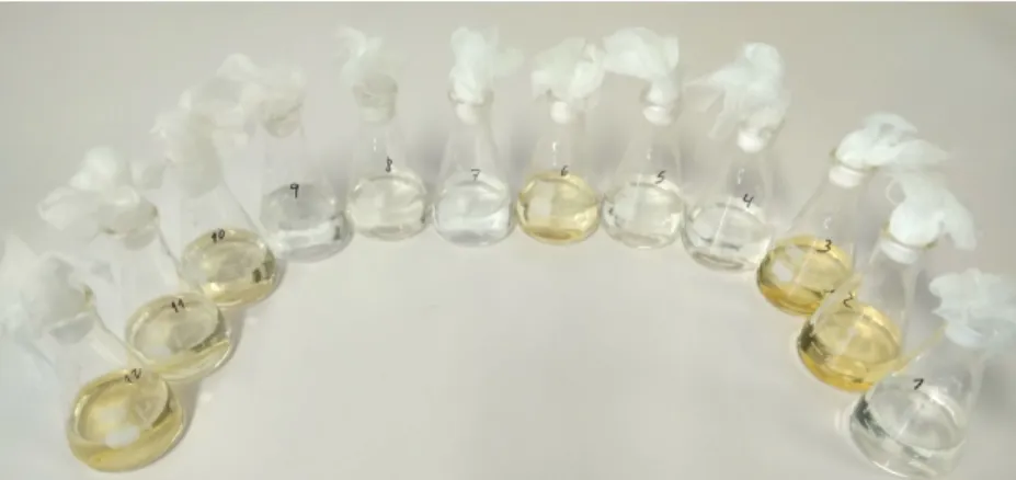
Figure 13 – Image obtained from the twelve batch reactors utilized in the first Experiment. ... 24
Figure 14 – Schematic representation of the experiment – Impact of the microplastics on the growth rate.37 Figure 15 - Schematic representation of the experiment – Changes in biodegradation with microplastics size. ... 37
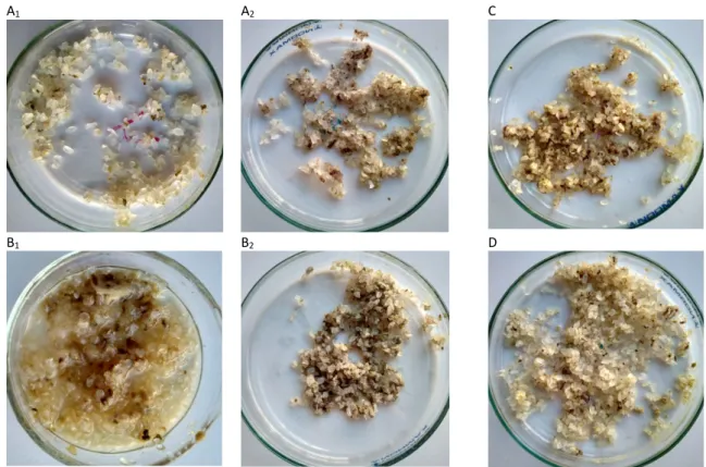
Figure 16 - Photos from microplastics covered with fungus biomass from the different tanks. The letters above each photo, identify from which tank the microplastics where recovered. ... 40
Figure 17 – Images obtained by SEM from a microplastic covered with fungus. ... 41
Figure 18 - FTIR-ATR spectra in the region 500 – 4000 cm-1 from samples of PE microplastics recovered in each tank, compared with a virgin PE microplastic. ... 42
Figure 19 – FTIR-ATR spectra in the region 500 – 4000 cm-1 from samples of PE microplastics recovered in each tank, compared with a virgin PE microplastic. ... 45
Figure 20 - FTIR-ATR spectra in the region 500 – 4000 cm-1 from samples of PE microplastics recovered in each tank, compared with a virgin PE microplastic. ... 48
Figure 21 – Molecular structure of PEF. ... 53
Figure 22 – Characteristic FTIR spectra of PEF. ... 53
Figure 23 -Schematic representation of the experiment to assess the capacity of Z. maritimum to biodegrade PEF microplastics. ... 54
Figure 24 - Schematic representation of the experiment to compare the capacity of Z. maritimum and N. vibrissa to biodegrade PEF microplastics. ... 55
Figure 25 – Infrared spectra in the region 500-4000 cm-1 from the PEF microplastics through the experiment. ... 58
Figure 26 - Infrared spectra in the region 500-4000 cm-1 from the PEF microplastics exposed to Zalerion maritimum. ... 61
Figure 27 - Infrared spectra in the region 500-4000 cm-1 from the PEF microplastics exposed to Nia vibrissa. ... 62
List of tables
Table 1 - Known microorganisms with the capacity of biodegrade polyethylene. ... 12
Table 2 – Uniform Design U12(43) matrix. ... 21
Table 3 – Matrix for a central composite design for three variables and a a=1.63. ... 22
Table 4 - Culture medium composition for the Uniform Design. ... 23
Table 5 - Culture medium for Central Composite Design. ... 23
Table 6 - Bioegradation results from UD. ... 25
Table 7 - Bioegradation results with CCD. ... 26
Table 8 - Tests of between subjects’ effects, when a linear model is considered for the first experiment with UD, where “df" stands for degree of liberty, “F” stands for F-value and “sig” for P-value. ... 27
Table 9 - Tests of between subjects’ effects for the first UD experiment, when a quadratic model is considered, where “df" stands for degree of liberty, “F” stands for F-value and “sig” for P-value. ... 27
Table 10 – Characterization for the model presented in Equation 3, where “df" stands for degree of liberty, “F” stands for F-value, “sig” for P-value, and “R” for correlation coefficient. ... 28
Table 11 - Tests of between subjects’ effects, when a linear model is considered for the second experiment with UD, where “df" stands for degree of liberty, “F” stands for F-value and “sig” for P-value. ... 29
Table 12 - Tests of between subjects’ effects for the second UD experiment, when a quadratic model is considered, where “df" stands for degree of liberty, “F” stands for F-value and “sig” for P-value. ... 29
Table 13 – Characterization for the model presented in Equation 4, where “df" stands for degree of liberty, “F” stands for F-value, “sig” for P-value, and “R” for correlation coefficient. ... 30
Table 14 - Tests of between subjects’ effects, when a linear model is considered for the first experiment with CCD, where “df" stands for degree of liberty, “F” stands for F-value and “sig” for P-value. ... 31
Table 15 - Tests of between subjects’ effects for the first CCD experiment, when a quadratic model is considered, where “df" stands for degree of liberty, “F” stands for F-value and “sig” for P-value. ... 31
Table 16 - Tests of between subjects’ effects, when a linear model is considered for the second experiment with CCD. where “df" stands for degree of liberty, “F” stands for F-value and “sig” for P-value. ... 32
Table 17 - Tests of between subjects’ effects for the second CCD experiment, when a quadratic model is considered, where “df" stands for degree of liberty, “F” stands for F-value and “sig” for P-value. ... 33
Table 18 - Medium composition and %degradation obtained through maximization for the CCD data. ... 34
Table 19 - Biomass and respective growth rate of Zalerion maritimum. ... 39
Table 20 – Relative areas from the identified regions from the microplastics spectra. ... 42
Table 21 - Carbonyl index for the analyzed samples. ... 43
Table 22 - Biomass and respective variation of Zalerion maritimum. ... 44
Table 23 - Microplastics in the beginning and at the end in each tank. ... 44
Table 24 - Relative areas from the identified regions from the microplastics spectra. ... 46
Table 25 – Carbonyl index of the analyzed samples. ... 46
Table 26 - Biomass and respective variation of Zalerion maritimum. ... 47
Table 27 - Microplastics in the beginning and at the end in each tank. ... 48
Table 28 - Relative areas from the identified regions from the microplastics spectra. ... 48
Table 29 - Carbonyl index of the analyzed samples. ... 49
Table 30 - Variation of fungus biomass throughout the experiment. ... 56
Table 31 – PEF microplastics at the beginning and at through the experiment. ... 57
Table 32 - Relative areas from the identified regions from the microplastics spectra. ... 58
Table 33 - Variation of Zalerion maritimum biomass throughout the experiment. ... 59
Table 34 - Variation of Nia vibrissa biomass throughout the experiment. ... 60
Table 35 – Variation of PEF microplastics before and after their exposure to Zalerion maritimum. ... 60
Table 36- Variation of PEF microplastics before and after their exposure to Nia vibrissa. ... 61
Table 37 - Relative areas from the identified regions from the microplastics spectra of 14 days exposed to N. vibrissa, a control and a virgin sample. ... 62
List of abbreviations
ASTM American Society for Testing and Materials CCD Central Composite Design
FDCA 2,5-furandicarboxylic acid
FTIR-ATR Fourier transform infra-red spectroscopy HDPE High density polyethylene
LDPE Low density polyethylene LLDPE Linear low-density polyethylene LMDPE Linear medium density polyethylene
NOAA National Oceanic and Atmospheric Administration
PE Polyethylene
PEF Poly(ethylene2,5-furandicarboxylate) PET Poly(ethylene terephthalate)
PHA Poly-3-hydroxyalkanoates PHB Poly[(R)-3-hydroxybutyrate] SEM Scanning electron microscopy SPI Society of the Plastic Industry UD Uniform Design
1. Introduction
1.1. Plastics in the marine environment
Marine litter is a major concern, since it is present in large quantities and spread throughout all oceans on Earth, having environmental, health and economic impacts1–3. The term marine litter encompasses different materials that were lost unintentionally or discarded in beaches, that were transported by rivers and winds from land to the seas, or that were disposed of directly in the oceans1.
One of the most common material found in marine litter is plastic, it is present in various sizes and shapes and has great impacts in the marine ecosystems1,3. For this reason, there is a growing demand for new ways to reduce them.
Plastics are a sub-category of polymeric material, produce by the polymerisation of units (monomers), making an organic synthetic long chain-like molecule, normally petroleum-based. It is possible to produce different types of plastics, depending on the monomers or on the additives add to the chain, and they can be divided in thermoset and in thermoplastics4,5. Thermosetting plastics are formed from a resin or soft solid or viscous liquid prepolymer, and they are resistible to heat, not losing their form with high temperatures6. Thermoplastics normally are produced in the form of beads, and them heated and moulded in the intended shape, and can be remoulded.
This kind of material is highly used, in different areas and their mass production start in 1950s5. Since then, they have helped to improve life quality, due to their properties, as their light, temperature, water and chemical resistant, but also because the manufacturing of plastic products is easy and has a low cost associated7.
Every year the production of plastics increases, in 2016 their production reached »335 million tonnes, and this large production creates big environmental problems5. As plastic are so resistant, they are also resistant to degradation in the nature, and the best way to reduce the plastic would be through recycling, but only 31.1% of plastics are recycled in Europe and 27.3% still go to the landfill1,5.
Microplastics were firstly reported in the 1970s, in a publication describing the potential impact of plastic on marine animals, where Carpenter and Smith8 refer the presence of small plastic particles inside the animals. Depending on the author, this term can have different definitions, which makes it difficult to analyse and compare different studies. Nowadays, some authors use the definition from the National Oceanic and Atmospheric Administration (NOAA). According to this organization, the term microplastics defines plastic debris with a size between 5mm and 1mm in size, and debris with less than 100 nm are called nanoplastics 9,10.
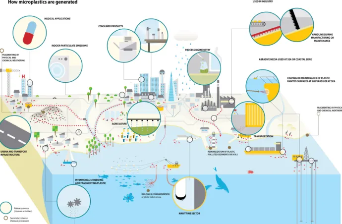
Microplastics, as represented in Figure 1, can be classified as primary microplastics or secondary microplastics, according to their origins. Primary microplastics are particles produced in this size, in the form of pellets, plastic-based granulates used in the cosmetics industry or in the form of a vector for drugs in medicine. Secondary microplastics are plastics debris, that result from the fragmentation of macro plastics, such as bottles or shopping bags. This fragmentation can be caused by different mechanisms, such as chemical and physical aging or degradation9,10.
Figure 1 – Schematic presentation of the sources of microplastics1 from Maphoto/Riccardo Pravettoni, available at
Carpenter and Smith8, in their paper also warn, for the first time, about the alarming presence of plastic pellets on the surface of the North Atlantic Ocean, in areas where dumping does not occur. These authors were unable to identify what kind of plastic the pellets were, but most of the samples would probably be polyethylene11. Later, in the same year, Carpenter et al12 reported the presence of two types of polystyrene pellets, a crystalline and an opaque form, in the coastal waters of southern New England. It is also referred that the opaque pellets were selectively consumed by the fish on that area. Since then the presence of plastic particles with every size has been reported, and in the past few years the interest in understanding how they end up in the ocean, how they suffer degradation and fragmentation, which are the impacts of their presence and how it would be possible to reduce them, has grown, being the topic of several papers11,13–15.
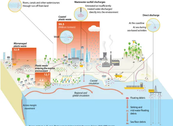
In 2015, Jambeck et al16 reported as estimate of the mass land-based plastic entering the ocean, based on data from solid waste and population density worldwide, and on the sources and main pathways of plastic into the oceans. The data was later resumed in Figure 2 by the Association GRID-Arendal1, to help better understand the problem itself.
Figure 2 – Microplastics’ pathways into the ocean1 from Maphoto/Riccardo Pravettoni, available at
As seen in Figure 2, plastic may enter the marine environment in multiple ways, by direct discharge in sea-based activities or at coastline, by the discharge of wastewater poorly treated or the discharged made by the industry, by rivers, canals or other sources that carry the mismanaged plastic waste. Due to their density and low weight the plastic will be carried by marine currents, as seen in Figure 3. That is why we may find plastic particles all around the globe, even in places with small population density like the Artic polar waters13,17 or in the Antarctic waters and sediments 18–20.
Figure 3 – Representation of the marine currents and the marine gyres1 from Maphoto/Riccardo Pravettoni, available at
http://www.grida.no/resources/6913.
Most of plastic particles are concentrated in mid-ocean gyres, as can be observed in Figure 3, and, more clearly, in Figure 4, with the help of the colours. This was described by Eriksen et al21. In this paper the authors, through sampling over the years and in different places, where able to estimate the number of particles and the total weigh of plastics in the ocean. They concluded that in the Northern Hemisphere the ocean regions contain 56.8% of plastic mass and 55.6% of particles, being the North Pacific the ocean with most plastic particles and contributes for 35.8% of the mass total. In the order hand, the Indian Ocean
is the region of the Southern Hemisphere with the higher number of particles and weight of plastics. These authors make this difference between mass and number, as microplastics normally contribute for the high number, but in mass terms are negligible, like evidenced by Lebreton et al22, that find that microplastics accounted for 94% of the particles plastic founded by them, but in mass represents only 8% of the total.
Figure 4 – Model of the amount of microplastics present in the marine environment and the mismanaged plastic particles available to enter in the oceans, retrieved from Zalasiewicz et al.15 with the permission of Elsevier.
Normally, the most abundant type of plastic found is polyethylene (PE), as reported by different authors, such as Sadri and Thompson23 that in a sampling on the Southwest of England found that 40% of the sampled plastics were PE , 25% were polystyrene (PS) and 19% were polypropylene. Zettler et al24 and Rios et al25 also found that PE and PS were the most abundant in their samples.
Since plastic particles are widely distributed in different areas of the marine environment, and have special characteristic, such as food smell26, they are commonly mistaken by food. For consequence, as it is illustrated in Figure 5, marine animals, like fishes, turtles, seagulls2 and others end up feeding on them.
Figure 5 – Schematic representation of the relation between microplastics and the marine animals1 from
Maphoto/Riccardo Pravettoni, available at http://www.grida.no/resources/6904.
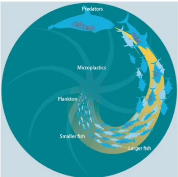
Microplastics, in specific, due to their small size, end up been ingested by all the animals in the food chain. In Figure 6 it is depicted the bioaccumulation effect, this occur because, as microplastics serve as food from zooplankton to big fishes, when a bigger animal feeds from a smaller animal with microplastics on the interior, it ends up ingesting more microplastics.
Figure 6 - Representation of the bioaccumulation effect of the microplastics1 from Maphoto/Riccardo Pravettoni,
Plastics, in general, when ingested by the animals, may have different physical or chemical impacts. Physical impacts are more associated with macroplastics, which can cause blockage of the digestive tract, which will lead to a reduction in food intake, starvation and loss of energy. However, microplastics can also cause blocking in the gut and changes in enzyme production, difficulty in breathing, reduce of vigour and mobility problems. Chemical impacts may be sublethal, when they alter animal behaviour, cause morphological changes and/or negative reproductive effects, or they may be lethal, when cause damage in central nervous system, cancer or death. Chemicals impacts are caused by the chemical composition of the plastics, but may also be caused by chemical contaminants adsorbed by plastics7,27.
As microplastics are found in some species intended for human consumption28,29, it is necessary to understand the possible impacts of their ingestion in human health. Some authors refer that, since microplastics are found in the digestive tract of the marine animals, parts not normally used in human diet, it is unlikely that their ingestion occur4, so the concern is unnecessary.
However, recent findings indicate that microplastics can also enter in the marine organisms without ingestion, when they are taken up by the gills, or when they transfer from the gastrointestinal tract to the circulatory system30–32. Additionally, microplastics have been found in other natural products like honey33 and sea salt34, as it is extracted from polluted waters, but also in processed products like beer35.
These evidences lead to the need for further investigation into the consequences of the consumption of microplastics on human health, but also ways of reducing microplastics in the marine environment3,29.
1.2. Degradation of plastics – types and definition
Degradation of plastics occur naturally, due to biotic and abiotic agents, or by their combination. This process is influenced by the characteristics of the polymers and it takes a long time, some studies indicate between 20 to 450 years, but it can also take more36. Unfortunately, it is still unclear whether, after the process of degradation, the polymers actually disappear, became too small to be seen or became other toxic components.
1.2.1. Abiotic Degradation 1.2.1.1. Chemical
Chemical degradation occurs when the properties of the plastic polymers are altered. These alterations can be caused by the oxygen, oxidative degradation, that breaks covalent bonds and produces free radicals. Can also be caused by the water, degradation by hydrolysis, that acts in specific groups, like esters, ethers, amides, anhydrides and ester amides, breaking their covalent bonds. This kind of degradation is influenced by the polymer’s structure, since an organised framework prevent diffusion of O2 and H2O, it occurs more easily in amorphous domains37.
1.2.1.2. Mechanical
Mechanical degradation is caused when a pressure is applied to the polymer and leads to a break, to a damage in the polymer chains. The compression or shear forces can be caused by air or water turbulence, by snow pressure, bird damage or ageing due to load37,38. This type of degradation normally, can only be seen at the molecular level.
1.2.1.3. Thermal
Thermal degradation is caused by oxidative reactions when plastics are overheated, resulting in its fusion, and leads to changes in the properties of the polymers, like reduction of weight and ductility or colour changes. In this kind of degradation two different reactions
occurs, random molecular scission of the long chain backbone and scission of C-C bonds ate the chain-end39.
This degradation hardly ever occurs in the nature, since the melting point of plastics are considerably higher than those observed in environmental conditions, but some plastics were developed with modifications in the composition, that make their melting point close to the environmental temperature37.
1.2.1.4. Photodegradation
Photodegradation changes the physical and optical properties of plastic materials and occurs due to oxidative reactions, caused by UV radiation and visible light. It acts mostly in the ether groups of soft elements, originating ester, aldehyde, formate and propyl end-groups, and if the UV radiation has sufficient energy, C-C bond cleavage can occur37,39. This degradation has been described as the most efficient in the nature, but some plastics were also developed, with specific groups to improve this type of degradation37.
1.2.2. Biodegradation
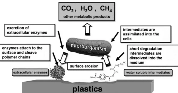
Biodegradation is defined in the ASTM standard D-5488-94d, (later replaced by the D-996-10a standard), as a “process which is capable of decomposition of materials into carbon dioxide, methane, water, inorganic compounds, or biomass in which the predominant mechanism is the enzymatic action of microorganisms, that can be measured by standard tests, in a specified period of time, reflecting available disposal conditions”40. This type of degradation will cause different changes on the plastic polymer, depending on the polymer and its previous biotic degradation, on the microorganism and on the environmental conditions37,38,41.
The biodegradation process, in biologic terms is yet to be fully understand, is still unclear all the enzymes involved, and the biological process involved when a microorganism uses a plastic polymer as subtract to grow. For now, some authors divide the process into three
different phases, first biodeterioration, followed by biofragmentation and finally assimilation. A schematic representation of biodegradation is pictured in Figure 7.
• Biodeterioration
This phase can be mechanical/physical, chemical or enzymatic, and it is characterized by the initial breakdown of the polymers in monomers. It occurs due to growth of microorganisms on the surface and/or inside the plastic material. Biodeterioration causes macroscopic alterations in the polymer, so is possible to estimate by appearance of holes and cracks and changes in colour37.
The physical way is based on the ability of microorganisms to secrete a complex matrix of polymers, which seep into the pores of the material and alter its moisture, heat transfer rates, pore size and distribution, which cause cracking, weakening the material. This matrix will also favour the penetration and development if the microorganisms, acting similarly to a surfactant, facilitating the exchanges between the hydrophobic and the hydrophilic phases37,38.
The biochemical biodeterioration is caused by the increase of microorganisms, which leads to an increase in the chemicals produced by their metabolism. Some of the acids released can react with the polymers’ components and increase erosion or can remove cations of the material, through oxidation reactions37.
The enzymatic process depends on the capacity of the microorganisms to produce enzymes, such as lipases, ureases or proteases. These enzymes bind to some type of polymers and catalyse the hydrolysis of specific bonds37,41.
• Biofragmentation
This phase is characterized by the cleavage and fragmentation of the monomers obtain previously, reducing their size. It is caused by enzymes, hydrolases (enzymatic hydrolysis) and oxidoreductases (enzymatic oxidation) or by radicular oxidation37,38.
Biofragmentation can be estimate by studying the presence of low molecular weight molecules, or by separating the oligomers obtained and analyse them37.
• Assimilation
This is the final phase, after the fragmentation the polymer´s fragments are small enough to be assimilated by the microorganisms, to pass through the membrane. They use the fragments as source of energy and elements, it works specially as their carbon source, to grow and reproduce. Some fragments are easily transported through the membrane, thanks to specific membrane carriers, but others need to undergo biotransformation into products that can directly assimilated37,38.
Figure 7 - Schematic presentation of the biodegradation’s mechanisms, retrieved from Mueller et al.42 with the
permission of Elsevier
1.2.2.1. Microorganisms involved in biodegradation
Different authors have already studied biodegradation, and demonstrated that various microorganisms, fungi and bacteria, have the capacity to degrade different types of plastics. Some of the microorganisms that were studied were found in environments with high proportion of plastic. In Table 1, some microorganisms already identified for the predisposition to biodegrade PE are listed. Their biodegradation capacity was, for some authors, studied in virgin plastic particles, i.e., plastics, that had not been subject to any environmental exposure, others in plastics that suffered a previous abiotic degradation, like photodegradation.
Table 1 - Known microorganisms with the capacity of biodegrade polyethylene. MICROORGANISM TYPE OF POLYETHYLENE REFERENCE
BACTERIA
Bacillus sp. PE 43,44
Bacillus pumilus PE 45,46
Bacillus pumilus LDPE 47
Bacillus mycoides PE 46
Bacillus amyloliquefaciens PE 46,48
Bacillus subitilis LDPE 47,49
Bacillus halodenitrificans LDPE 45
Bacillus circulans LDPE 50
Bacillus brevies LDPE 50
Bacillus sphericus LDPE 50
Staphylococcus xylosus PE 46
Staphylococcus epidermis LDPE 51
Rhodococcus rhodochrous PE 52
Rhodococcus ruber PE 53
Pseudomonas fluorescens PE 46
Pseudomonas aeruginosa LDPE 54
Bacillus cereus PE 45,46
Paenibacillus macerans PE 46
Micrococcus lylae PE 46
Nocardia asteroides PE 52
Enterobacter asburiae PE 43,44
Burkholderia seminalis LDPE 54
Stenotrophomonas pavanii LDPE 54
Brevibaccillus borstelensis LDPE 55
Lysinibacillus xylanilyticus LDPE 56
Kocuria palustris LDPE 47
Arthobacter paraffineus LDPE 57
FUNGI
Aspergillus flavus LDPE 58
Aspergillus flavus HDPE 59
Aspergillus awamori PE 46
Aspergillus versicolor PE 60
Aspergillus niger LDPE 56,61
Aspergillus tubingensis HDPE 59
Cunning-hamella sp. PE 46
Mucor sp. PE 46
Penicillum sp. PE 46
Penicillium simplicissimum PE 62
Penicillium pinophilum LDPE 61,63
Gliocladium viride PE 46 Mortierella subtlissima PE 46 Cladosporium cladosporoides PE 52 Zalerion maritimum PE 64 Acremonium kiliense PE 60 Verticillium lecanii PE 60
Gliocladium virens LDPE 61
Phanerochaete chrysosporium LDPE 61,65
Considering the wide presence of microplastics and their impacts, and the biodegradation capacity of this microorganisms, this study aims to:
• Optimize a culture medium in order to maximize the response in terms of removal of microplastics (Chapter 2)
• Enhance the volume of experience in order to ascertain if under non-sterilized conditions and environmental exposure the biodegradation of microplastics still occur (Chapter 3)
• Assess the capacity of fungi (Zalerion maritimum and Nia vibrissa) to biodegrade a bioplastic (Chapter 4)
2. Optimization of the experimental conditions for the biodegradation of polyethylene microplastics by marine fungi
2.1. Introduction
In a previous work, it has been demonstrated that Zalerion maritimum was able to biodegrade PE microplastics64, which shows that this can be a solution to the problem of (micro)plastics in the environment. In this work, it was also shown that biodegradation is influenced by the biomass grow and therefore by the culture medium conditions. Thus, the need of optimization of the experimental conditions was evident after an initial experiment (see Appendix A) where Z. maritimum was unable to grow and to biodegrade PE microplastics in a culture medium with a reduced nutrient content. Our biodegradation experiment is based on the idea that Z. maritimum can use microplastics as carbon source, being necessary to supplement, in the culture medium, the rest of the nutrients required for the growth of the fungus. Therefore, this study aims at establishing the optimum experimental conditions for the biodegradation of PE microplastics by Z. maritimum using statistical design of experiments.
The medium optimization involves five steps, (1) statistic design of the experiments; (2) experimental procedure; (3) analyses of the results with a statistical software; (4) perform a regression to estimate the coefficients of a mathematical model, where all variables and correlation between them are considered, Equation (1) - Correlation between response (Y) and independent factors, where !" represent the intercept and ! represent the coefficient
values; (5) with the help of the mathematical model determine the optimal values66,67.
# = !"+ & !'(' ) '*+ + & !''('', ) '*+ + & & !'-(' ) .-*+ ( -) '*+ + / Eq (1)
Two different experimental design were used, Uniform Design and Central Composite design, in order to compare the results and understand which one would be better, would give a more appropriate model. The three medium components, glucose, malt extract and
peptone were considered as independent factors or variables and the degradation percentage of PE microplastics was considered as response.
2.1.1. Uniform Design (UD)
UD is an experimental design developed by Fang and Wang in 199468, based on a number theory, where the design points scatter uniformly on the experimental domain. This experimental design was chosen, since within a small number of experiences is possible to obtain a great amount of information, as well as explore the relationships between the factors and the response68. UD also performs correctly even when the regression model is unknown68. The number of experiments is influenced by the number of factors and levels for each factor and is given by tables developed with the theory.
This experimental design has been successfully used in different fields since the 1980s. In the microbiology, authors as Xu et al69, Chen et al70, Li et al71 and Mu et al72, have already used UD as experimental design, to optimize a culture medium, for growth, for degradation or production of a compounds.
2.1.2. Central Composite Design (CCD)
CCD, also called Box-Wilson Design, was introduced by G.E.P. Box and K.B. Wilson in 195173. This experimental design has been widely used in different areas for the optimization of experimental conditions, and in the case of microbiology, its use had already been reported by Sadhukhan et al.74, Adinarayana et al.75, Ooijkaas et al.76 and Ibrahim et al.77, for the optimization of conditions for the production or degradation of a specific compounds. For been widely used it was chosen as comparison term.
The number of experiments is given by the Equation 2, where 21 represents the number
of two-level factorial or fractional factorial design points, all the possible combinations pf +1 and -1 levels of factor; and 22 represents the number of axial points (star points), points with a fixed distance (a) from the center; and 2 is be the number of center points, and represents the replicate terms, which provide an estimation of the experimental error.
2.1.3. Zalerion maritimum
Zalerion maritimum (or Zalerion maritima), the studied fungi, is a marine fungus belonging to the Ascomycota phylum78,79, defined in 1963 by Anastasiou 80, but first described in 1944, as Helicoma maritimum by Linder 81. This change was due to the fact that Anastasiou noticed that the species Helicoma salinum, also described by Linder in 1944, and the species Zalerion nepura, Zalerion eistla, Zalerion xylestrix, Zalerion raptor, described by Moore and Meyers in 1962, belonged to the same species being strains of Zalerion maritimum 80.
This fungus is a member of the subphyla Pezizomycotina78,79, that includes all filamentous fungi with a fruiting body, visible to the naked eye, it belongs to the Sordariomycetes78,79 class characterized by their perithecial ascomata and inoperculate unitunicate asci, where the ascospores are contained82–84. It also belongs to the Lulworthiales order and to the Lulworthiaceae family78,79 being a marine fungus that grows on submerge wood which can be characterized by its brown to black ostiolate ascomata, hyaline and filamentous ascospores and thin-walled asci85,86.
Zalerion maritimum is one of the only reported anamorphs, name of the species at the asexual form in the Lulworthiales order being a hyphomycete and present a coiled conidia, his teleomorph is Lulwoana uniseptata (or Lulworthia uniseptata), the name of the species in the sexual reproductive stage87–89.
In various studies from the 1970s and from the 1980s, this fungus showed ability to degrade different components. Henningsson and later Sutherland and Crawford, demonstrated that Z. maritimum is able to degrade lignin, to CO2 and water-soluble products, in both hardwood and softwood lignocelluloses90.
Sguros and Quevedo, studied the predisposition of this fungus to use Aldrin and Dieldrin as subtract, concluding that Z. maritimum can degraded both compounds under marine conditions and used it to grow91. Aldrin and Dieldrin are two pesticides highly used between the 1950s and 1990s, developed as an alternative to DDT (Dichlorodiphenyltrichloroethane), they were highly resistant in the environment and
despite not been hydrophobic and don’t dissolve easily in water, they were the pesticides most detected in rivers and dieldrin, for instance was presented in watersheds. As any chemical pollutant, they have negative consequences in the organisms, been biomagnified along the food chain and they were linked to health problems in humans92,93.
Jones and Le Campion-Alsumard, found polyurethane coatings submerged in the sea were colonized with four different fungi, Z. maritimum was one of them94. This article from 1968, already show the predisposition of this fungus to biodegrade plastics, as Z. maritimum was able to form a biofilm on this plastic polymer. Some studies support this, as showed that polyester based on polyurethane were vulnerable to fungus attack.
Other important function of Z. maritimum was discovered in 1973, by Catalfomo et al, they reported Z. maritimum as one of the marine fungi able to produce Choline sulfate95. Molina and Hughes96 showed that Z. maritimum is able to live in a wide range of temperatures, from 5ºC to 40ºC, and in different salinity conditions, from 0 to 99.9‰. According to their study the fungus can live in conditions of extremes temperatures, if the salinity is higher. Previous studies corroborate this idea, and also the optimal temperature found buy the authors, between 20ºC and 25ºC96,97. Other important thing, described by these authors, it is that the fungus is able to adapt to the different conditions, but with repeated transfers in a same medium type a selection of physiological races can occur96,97. The medium pH is optimum at 7.5, but the fungus can show growth in a great range of pH, according to Churchland and McClaren’s98 findings, the fungus’ mycelium changes color depending on the pH of the medium. In their experiments, the mycelium stayed beige in low-pH medium and became black in all other solutions96–98, this also happens depending on the nutrients source.
Due to its great adaptability to the medium is possible to encounter this species in different locations. Studies report their present along all European coast99,100, in the Canadian98 coast and Malaysian coast101. Their anamorph has been reported in the Japan coast88.
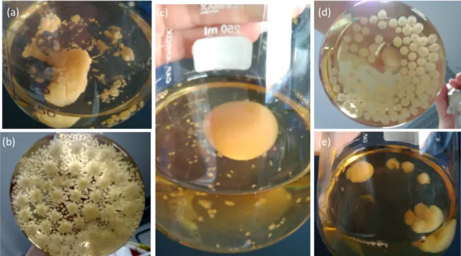
Figure 8 – Photos from the different forms that Zalerion maritimum presented in our laboratory. In (a) and (e) Z.
maritimum presents an irregular form; figure (b) presents a form that resembles a star, due to sporulation; (c) and (d)
present the fungus in its globular form.
2.1.4. Polyethylene (PE)
As the most widely produced polymer in the world, PE, seems to be also the most found polymer worldwide in the marine environments.
This polymer was accidentally discovered in 1933 by Eric Fawcett and Reginal Gibson as they tried to condense at high pressure and temperature, ethylene with benzaldehyde. In this “accident” they obtained a residue that was PE, but later failed to repeat the experiment successfully, so it was not until 1935 that chemist Michael Perrin was able to obtain large amounts of PE, using ethylene with traces of oxygen102–104.
In 1939, the commercial production of high-pressure polyethylene, now known as low-density polyethylene, began and was widely used during the World War II. In the following years, different advances in production were made, in the manufacturing or in base products, until we reached the parameters used today102–104. It has become the most globally produced and widely used synthetic polymer, since as a thermoplastic, it can be melted and shaped into primary form and later reshaped into various forms and devices,
(a)
(b)
(c) (d)
and also because it has excellent chemical resistant and it is the cheapest plastic polymer to manufacture5,105.
This plastic have a linear formula (H(CH2CH2)nH), Figure 9, and a melt index of 1.0g/10 min (190oC/2.16kg). It is obtained by the polymerization of Ethylene (CH2=CH2), a simplest olefin, through the action of initiators and catalysts. The conditions for polymerization, can vary and will influence the composition, structure and properties of the polymer, existing a wide range of PE available in the industry102–104.
Figure 9 – Molecular representation of PE monomers.
This leads to the need for a grading system that differentiates the different types of PE. Based on the crystallinity, and consequently in the different densities, Society of the Plastic Industry (SPI) identified three main categories to define this plastic: Low density 0.910-0.925 g/cm3; Medium density 0.926-0.940 g/cm3; High density 0.941-0.965 g/cm3. The American Society for Testing and Materials (ASTM), has also defined types of PE, but more stringently, with five categories: High density polyethylene (HDPE) >0.941 g/cm3; Linear medium density polyethylene (LMDPE) 0.926-0.940 g/cm3; Medium density polyethylene (MDPE) 0.926-0.940 g/cm3; Linear low-density polyethylene (LLDPE) 0.919-0.925 g/cm3; Low density polyethylene (LDPE) 0.910-0.925 g/cm3. Some manufactures have their own classifications and nomenclatures, since classifications can’t only be based on their density, is necessary classifications based on molecular weight or comonomer employed102,105.
(a) (b)
2.2. Materials and Methods 2.2.1. Microplastics
Polyethylene pellets were approximately 2-4mm in size and exhibited spheroid morphology. The pellets were acquired from Sigma-Aldrich (USA) and mechanically cut to obtain microplastics with a size range 1000 μm < MP < 250 μm, defined with the help of sieves. Microplastics were characterized both by Optical, Figure 11(a), and Scanning electron microscopy, Figure 11(b) e (c), and also by Fourier transform infra-red spectroscopy, Figure 12. PE have characteristic peaks, as seen in Figure 12, between 2980-2800 cm-1, 1500-1400 cm-1 and 750-650 cm-1, caused by CH2 asymmetric and symmetric stretching, bending and rocking deformations106.
(a)
(b) (c)
Figure 11 - Optical (a) and electron microscopy (b) and (c) images of the microplastic and its surface
Figure 12 – FTIR spectra characteristic for a PE microplastic.
0 0,1 0,2 0,3 0,4 0,5 0,6 500 1000 1500 2000 2500 3000 3500 4000 Ab so rb an ce Wavenumber (cm-1)
2.2.2. Microorganism
Zalerion maritimum (ATTC 34329, American type culture collection), was maintained in culture in our laboratory, in recommended conditions for growth107, 2/3 weeks in a culture medium with the composition of 35 g/L of salt, 20 g/L of glucose, 20 g/L of malt extract and 1 g/L of peptone and temperatures around 20oC.
2.2.3. Design of experiments and Statistical analysis
MINITAB software was used to obtain the tables for the CCD experiments, and to analyse the data generated by that experiments, through linear regression and maximization analysis.
SPSS software was used to do statistical analyses, like the study of statistically significance of each variable, on the data from both experimental designs.
A second-order polynomial regression equation was also obtained through SPSS software analysis for UD experimental data. The optimal conditions were obtained by solving the equation the help of WolframAlph website.
2.2.3.1. Uniform Design
For this experimental design were defined four levels for each factor, and twelve runs, obtaining a U12(43) matrix, as seen in Table 2.
Table 2 – Uniform Design U12(43) matrix.
RUN ORDER X 1 X 2 X 3 1 3 2 2 2 3 4 4 3 4 4 2 4 4 1 4 5 2 2 3 6 1 3 4 7 2 1 1 8 4 2 1 9 1 1 3 10 3 3 3 11 2 3 2 12 1 4 1
2.2.3.2. Central Composite Design
In this experimental design, five levels for each factor were considered: -a, -1, 0, +1, +a, the design generated, can be seen in Table 3.
Table 3 – Matrix for a central composite design for three variables and a a=1.63.
STDORDER RUNORDER PTTYPE BLOCKS X 1 X 2 X 3
15 1 0 1 0 0 0 6 2 1 1 1 -1 1 18 3 0 1 0 0 0 1 4 1 1 -1 -1 -1 4 5 1 1 1 1 -1 3 6 1 1 -1 1 -1 20 7 0 1 0 0 0 11 8 -1 1 0 -1.63 0 14 9 -1 1 0 0 1.63 17 10 0 1 0 0 0 2 11 1 1 1 -1 -1 5 12 1 1 -1 -1 1 12 13 -1 1 0 1.63 0 16 14 0 1 0 0 0 9 15 -1 1 -1.63 0 0 19 16 0 1 0 0 0 13 17 -1 1 0 0 -1.63 7 18 1 1 -1 1 1 8 19 1 1 1 1 1 10 20 -1 1 1.63 0 0 2.2.4. Culture medium
The culture medium was composed by 35 g/L of salt108, this was maintained fixed as it is necessary to keep the necessary salinity for the fungi, and simulate the salt water.
It was also composed by the factors to be optimized, glucose109, malt extract110 and peptone111, and their concentration varied accordingly to the experimental designs characterized previously, as seen in Table 4 and Table 5.
Table 4 - Culture medium composition for the Uniform Design.
RUN ORDER GLUCOSE
(G/L) MALT EXTRACT (G/L) PEPTONE (G/L)
1 10 2 0.1 2 10 20 1 3 20 20 0.1 4 20 0 1 5 2 2 0.5 6 0 10 1 7 2 0 0 8 20 2 0 9 0 0 0.5 10 10 10 0.5 11 2 10 0.1 12 0 20 0
Table 5 - Culture medium for Central Composite Design.
RUN ORDER GLUCOSE
(G/L) MALT EXTRACT (G/L) PEPTONE (G/L)
1 12.5 12.5 0.7 2 20 5 1 3 12.5 12.5 0.7 4 5 5 0.4 5 20 20 0.4 6 5 20 0.4 7 12.5 12.5 0.7 8 12.5 0 0.7 9 12.5 12.5 1.2 10 12.5 12.5 0.7 11 20 5 0.4 12 5 5 1 13 12.5 25.1 0.7 14 12.5 12.5 0.7 15 0 12.5 0.7 16 12.5 12.5 0.7 17 12.5 12.5 0.2 18 5 20 1 19 20 20 1 20 25.1 12.5 0.7
2.2.5. Experimental conditions
The first experiment, based on Uniform Design, was performed using twelve batch reactors (50ml Erlenmeyer flask) with 30 mL of culture medium and approximately 0.010 g of microplastics. All batch reactors were autoclaved and later inoculated with approximately 0.30 g of fungus mycelium.
A second experiment, based on Central Composite Design, was performed using twenty batch reactors (this time 100mL Erlenmeyer flask) with 60 mL of culture medium and 0.020g of microplastics. The batch reactors were autoclaved and then inoculated with 0.60g of fungus mycelium.
A third experiment was realized, where thirty-two batch reactors (also 100 mL Erlenmeyer flask) were utilized, twelve of then had their culture medium based on Uniform Design and twenty of them had their culture medium based on Central Composite Design, so the experiments could be performed at the same time, and easier compared. Each batch reactor had 50 mL of a specified medium and 0.015g of microplastics, and was autoclaved and afterwards inoculated with 0.50g of fungus mycelium.
After inoculation, in all three experiments, the batch reactors were maintained for 30 days in a shaker, at room temperature and with stirring at 120 rpm. At the end the fungus and the microplastics were separated from the medium by filtration. The fungus biomass was retrieved and posteriorly frozen and lyophilized. The microplastics were kept for weighing and further analysis. The lyophilized biomass was also examined for the presence of microplastics, which may have not been completely degraded.
2.3. Results and discussion
Table 6 and Table 7 present the percentages of microplastics removed obtained in the experiments based on Uniform design and Central composite design, respectively. In Table 6, some data are missing, because due to contaminations it was not possible to recover that data and therefore were disregarded. Table 7 present all values, but some Erlenmeyer also had contaminations that may have slightly altered the fungus behavior, which may explain the variation between the value obtained in the first experiment and those from the second experiment, for example, in the case of sample 4 or sample 12.
According to both tables, in each experiment, the percentages of microplastics removed varied, approximately, from 0% to 94%. This wide variation proves the importance of a medium optimization to achieve a higher degradation.
In both cases, it was possible to observe that the results are not the same in the first and second experiments. This variation can be explained by different situations beside contaminations, like the fact that the fungi may had behave differently, as they are biological replicas and also by the fact that the experiments did not occur at the same time.
Table 6 - Bioegradation results from UD.
UNIFORM DESIGN % MICROPLASTICS REMOVED
RUN ORDER First Exp. Second Exp.
1 7.20 27.27 2 72.73 75.32 3 86.67 94.81 4 37.30 74.51 5 40.78 35.48 6 73.83 31.61 7 - 28.00 8 0.00 34.21 9 36.67 14.10 10 87.50 57.05 11 71.65 92.26 12 72.36 -
Table 7 - Bioegradation results with CCD.
CENTRAL COMPOSITE DESIGN % MICROPLASTICS REMOVED
RUN ORDER First Exp. Second Exp.
1 88.00 69.62 2 70.48 69.48 3 86.54 78.98 4 6.67 44.97 5 72.73 73.68 6 76.00 91.77 7 85.24 78.00 8 34.55 19.33 9 85.83 60.53 10 72.11 50.00 11 94.07 76.10 12 40.00 83.55 13 93.16 74.50 14 81.85 66.88 15 52.27 37.82 16 88.57 78.06 17 87.78 71.14 18 73.33 87.10 19 67.00 36.67 20 79.47 78.95
2.3.1. Effect of different medium compounds on polyethylene’s biodegradation 2.3.1.1. Uniform Design
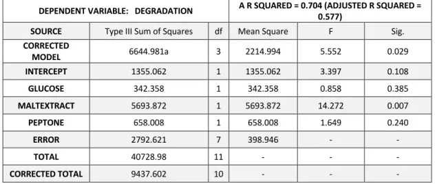
In Table 8 is presented the results from the analysis of covariance, if a linear model is considered, based on that table is possible to conclude that “malt extract” is the most significant factor, the compost that more influence the percentages in the biodegradation of PE microplastics. However, based on this table, is also possible to understand that a linear model is not the best suitable, since adjusted R2 is just 0.577.
Table 9 present the test between subjects when all interactions between the factors are considered. In this case, the adjusted R2 is 0.961 which indicates a high significance of the model, but none of the factor seen to be important, since all “sig” values are higher than 0.05. This means that a regression analysis is necessary in order to find a model with a
better fit. Despite that, “malt extract” stays the most important factor, as its “sig” value is the smaller and closer to 0.05.
Table 8 - Tests of between subjects’ effects, when a linear model is considered for the first experiment with UD, where “df" stands for degree of liberty, “F” stands for F-value and “sig” for P-value.
DEPENDENT VARIABLE: DEGRADATION A R SQUARED = 0.704 (ADJUSTED R SQUARED = 0.577)
SOURCE Type III Sum of Squares df Mean Square F Sig.
CORRECTED MODEL 6644.981a 3 2214.994 5.552 0.029 INTERCEPT 1355.062 1 1355.062 3.397 0.108 GLUCOSE 342.358 1 342.358 0.858 0.385 MALTEXTRACT 5693.872 1 5693.872 14.272 0.007 PEPTONE 658.008 1 658.008 1.649 0.240 ERROR 2792.621 7 398.946 - - TOTAL 40728.98 11 - - - CORRECTED TOTAL 9437.602 10 - - -
Table 9 - Tests of between subjects’ effects for the first UD experiment, when a quadratic model is considered, where “df" stands for degree of liberty, “F” stands for F-value and “sig” for P-value.
DEPENDENT VARIABLE: DEGRADATION A R SQUARED = 0.996 (ADJUSTED R SQUARED = 0.961)
SOURCE Type III Sum of Squares df Square Mean F Sig.
CORRECTED MODEL 9400.633a 9 1044.515 28.253 0.145
INTERCEPT 0.134 1 0.134 0.004 0.962 GLUCOSE * GLUCOSE 99.209 1 99.209 2.684 0.349 PEPTONE * PEPTONE 243.335 1 243.335 6.582 0.237 MALTEXTRACT * MALTEXTRACT 1020.319 1 1020.319 27.599 0.120 GLUCOSE * MALTEXTRACT 45.414 1 45.414 1.228 0.467 GLUCOSE * PEPTONE 130.221 1 130.221 3.522 0.312 MALTEXTRACT * PEPTONE 27.459 1 27.459 0.743 0.547 GLUCOSE 131.89 1 131.890 3.568 0.310 MALTEXTRACT 2782.518 1 2782.518 75.265 0.073 PEPTONE 289.803 1 289.803 7.839 0.218 ERROR 36.969 1 36.969 - - TOTAL 40728.98 11 - - - CORRECTED TOTAL 9437.602 10 - - -
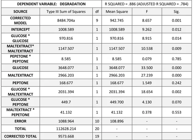
The regression analysis was done by successively removing the factors with the high “sig” value. For example, based on Table 9, the “malt extract*peptone” interaction and “glucose*malt extract” interaction, can be removed obtaining the Equation (3). As it can be
removed, it implies that these two interactions do not influence, as much as the others, the degradation. According to the coefficients used in the equation, the concentrations of peptone and malt extract influence positively the degradation, which means that with a higher concentration of this compound, high percentages of degradation of PE microplastics occur. On the other hand, the glucose concentration negatively affects the degradation, so a lower concentration of glucose is necessary to obtain higher degradation percentages.
According to the characterization, presented in Table 10, of Eq. (3), it is a model with good fit to the experimental data and a high significance, as its “sig” value is 0.007, and R adjusted is 0.960, meaning that 96% of the data is explained by this model.
%5678959:;<2 =
= −5.179 − 5.029 ∗ 7EFG<H6 + 149.773 ∗ K6K:<26 + 10.236 ∗ M9E: 6(:89G: + 0.0229 ∗ 7EFG<H6,− 143.752 ∗ K6K:<26,
− 0.314 ∗ M9E: 6(:89G:, + 2.224 ∗ 7EFG<H6 ∗ K6K:<26
Eq. (3)
Table 10 – Characterization for the model presented in Equation 3, where “df" stands for degree of liberty, “F” stands for F-value, “sig” for P-value, and “R” for correlation coefficient.
MODEL SQUARES SUM OF DF SQUARE MEAN F SIG. R R2 ADJUSTED
R 1
Regression 9325.138 7 1332.163 35.536 0.007 0.994 0.988 0.960
Residual 112.464 3 37.488 - - - - -
Total 9437.602 10 - - - -
Table 11 present the results from an analysis of covariance to the results from the second experiment with UD, if a linear model is considered. Based on that table is possible to conclude that the “malt extract” is the most significant factor, “sig”<0.05, which is in agreement with the findings in the previous experiment. Also, as in the previous experiment, the linear model is not suitable, since adjusted R2 is only 0.382.
A test between subjects considering all interactions between the factors is presented in Table 12. In this case, the adjusted R2 is 0.865 which indicates a significance of the model, but similar to the other case, none of the factor seen to be important, since all “sig” values are higher than 0.05 and so a regression analysis is necessary. The “malt extract” factor also, remains as the most important, as its “sig” value is the smaller and closer to 0.05.
Table 11 - Tests of between subjects’ effects, when a linear model is considered for the second experiment with UD, where “df" stands for degree of liberty, “F” stands for F-value and “sig” for P-value.
DEPENDENT VARIABLE: DEGRADATION A R SQUARED = 0.567 (ADJUSTED R SQUARED = 0.382)
SOURCE Type III Sum of Squares df Mean Square F Sig.
CORRECTED MODEL 4851.360a 3 1617.120 3.060 0.101 INTERCEPT 1626.773 1 1626.773 3.078 0.123 GLUCOSE 801.26 1 801.260 1.516 0.258 MALTEXT 3081.478 1 3081.478 5.831 0.046 PEPTONA 0.404 1 0.404 0.001 0.979 ERROR 3699.088 7 528.441 - - TOTAL 36790.427 11 - - - CORRECTED TOTAL 8550.448 10 - - -
Table 12 - Tests of between subjects’ effects for the second UD experiment, when a quadratic model is considered, where “df" stands for degree of liberty, “F” stands for F-value and “sig” for P-value.
DEPENDENT VARIABLE: DEGRADATION A R SQUARED = 0.987 (ADJUSTED R SQUARED = 0.865)
SOURCE Type III Sum of
Squares df Square Mean F Sig.
CORRECTED MODEL 8435.367 9 937.263 8.144 0.266 INTERCEPT 608.944 1 608.944 5.291 0.261 GLUCOSE * GLUCOSE 202.109 1 202.109 1.756 0.412 MALTEXTRACT * MALTEXTRACT 2.403 1 2.403 0.021 0.909 PEPTONE * PEPTONE 107.053 1 107.053 0.930 0.512 GLUCOSE 163.214 1 163.214 1.418 0.445 MALTEXTRACT 1120.758 1 1120.758 9.739 0.197 PEPTONE 1.687 1 1.687 0.015 0.923 GLUCOSE * MALTEXTRACT 123.129 1 123.129 1.070 0.489 GLUCOSE * PEPTONE 688.249 1 688.249 5.981 0.247 MALTEXTRACT * PEPTONE 24.161 1 24.161 0.210 0.726 ERROR 115.081 1 115.081 - - TOTAL 36790.427 11 - - - CORRECTED TOTAL 8550.448 10 - - -
The regression analysis was done by removing the factors with the highest “sig” value, for example, based on table 12, it was removed the “malt extract2”, “peptone” and “peptone*malt extract” interaction, obtaining the Equation (4), characterized in table 13. In agreement with the first experiment based on UD, the interaction “peptone*malt extract” does not seem to be relevant, the concentration of glucose has a negative effect